
State Tracking and Fault Diagnosis for Dynamic Systems Using Labeled Uncertainty Graph


Abstract
:1. Introduction
- The Fault Detection and Isolation (FDI) methods capture system behavior using differential equation models, whose foundations are based on control and statistical decision theories.
- The Diagnosis (DX) methods use qualitative model and logical approaches, with foundations in the fields of computer science and artificial intelligence.
2. Theoretical Background
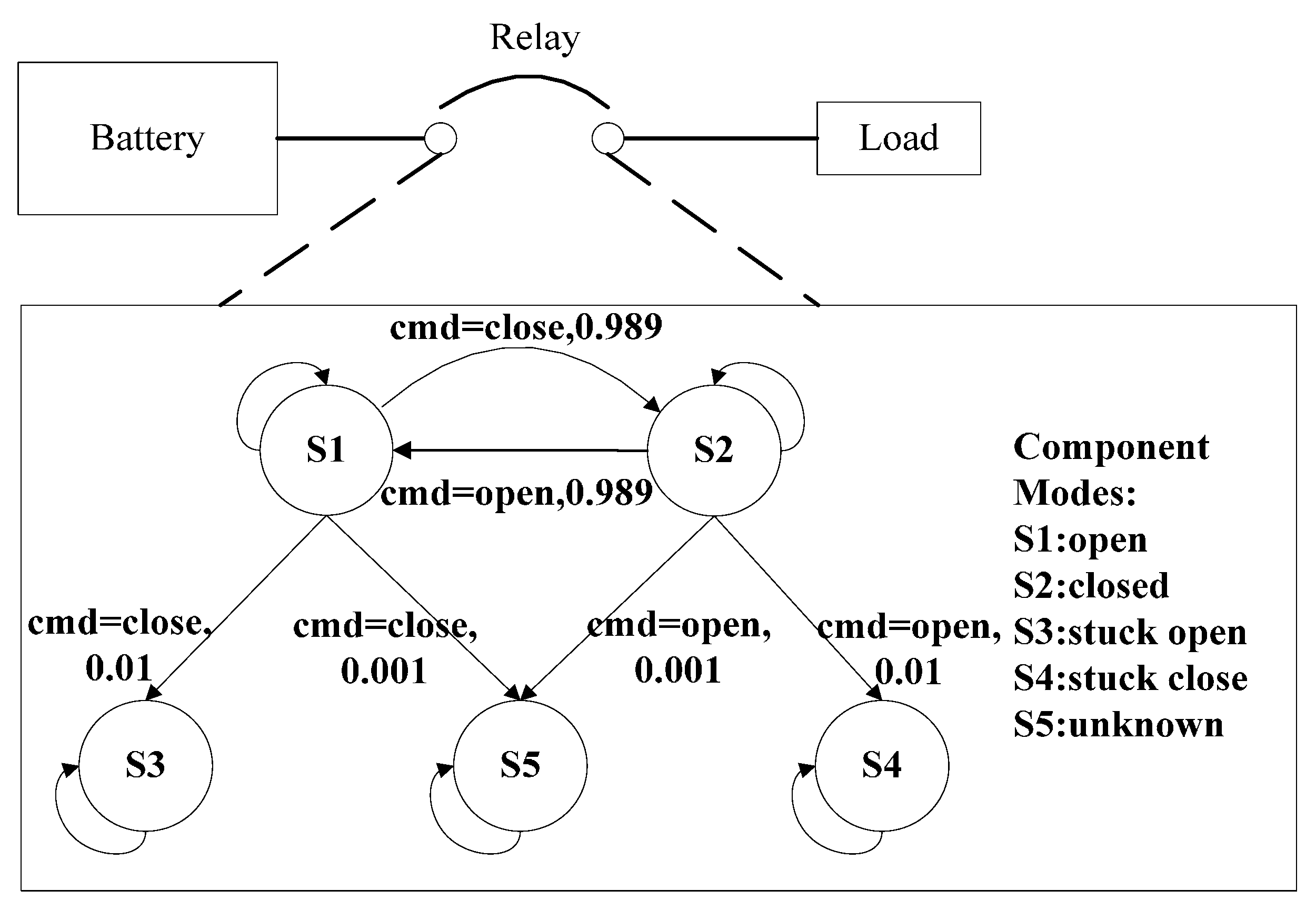
2.1. Component and System Model
- CV (component variable) is a set of variables for component i. It can be partitioned into mode variables, command variables and attribute variables. Mode variables define the possible behavioral modes for component. Command variables are the external controlled signals. Attribute variables include inputs, outputs and any other variables used to define the behavior of the component.
- CS (component constraint) is a set of formulas constraints, which consists of mode constraints and other constraints. Mode constraints define the physical behavior in certain mode. Other constraints denote the remaining unchanged constraints i.e., structure constraints.
- (transition relation) is denoted as a tuple from time t to time t + 1. and are the mode assignment at time t and t + 1, respectively. Guard is the transition event. Some events are observable (e.g., commands issued from external actuator), while the rest are unobservable (e.g., autonomous or fault events). Prob is a transition probability from to .
2.2. Simulation-Based Dynamic Diagnosis
- G is an entire system model.
- is the initial belief state, which is constituted by the mode for each component at time step 0.
- is a observation sequence , where are the observation variables or command variables at time step t.
2.3. Classical Belief State Update
3. Exploitation of LUG for State Tracking and Fault Diagnosis
4. Proposed State Tracking and Fault Diagnosis Algorithm
4.1. One Step Look-Ahead

| Loop | Path | Number of Particles | |||
|---|---|---|---|---|---|
| 1 | 0.989 | 0 | 0 | 0 | |
| 2 | 0.01 | 1 | 0;0.91 | 182 | |
| 3 | 0.001 | 1 | 0;0.91;0.09 | 18 |
4.2. Description of the Approach
- A fast roll forward process that uses the forward propagation to extract the likely belief states at each time-step.
- A quick roll back process using tagged particles to generate the possible trajectories.
| Algorithm 1: Roll forward process |
1: Input: Initial belief state ; Number of the particles N 2: Output: LUG with the most likely belief state at each time step 3: Sample N particles using the prior probability distribution 4: Add the initial belief state to proposition layer 5: For each time-step t >0 do 6: For each belief state in do 7: If all the particles can be assigned according to a set of obtained a posteriori transitions probability Then break 8: Execute possible transitions and store the corresponding effect into 9: If the successor belief state is consistent with observation 10: Save the belief state into proposition layer 11: Calculate the a posteriori transitions probability 12: Insert into a set of obtained a posteriori transitions probability 13: Else 14: Recalculate the normalization term 15: Update the set of obtained a posteriori transitions probability 16: End If 17: End For 18: Assign the particles for the belief state in according to a set of obtained a posteriori transitions probability 19: End For |
| Algorithm 2: Roll back process |
1: Input: Label uncertainty graph LUG
2: Output: A set of possible trajectories
3: For each time-step t>0 do
4: For each belief state in proposition layer do
5: For each particle in belief state do
6: Extract the belief state in which also contains the same particle
7: Roll back to generate the trajectory from to
8: Construct a new trajectory tuple
9: Add into obtained most likely trajectories
10: Merge the same trajectory and update the weight
11: End For
12: End For
13: End For
|
4.3. Analysis of the Approach
4.3.1. Correctness and Incompleteness
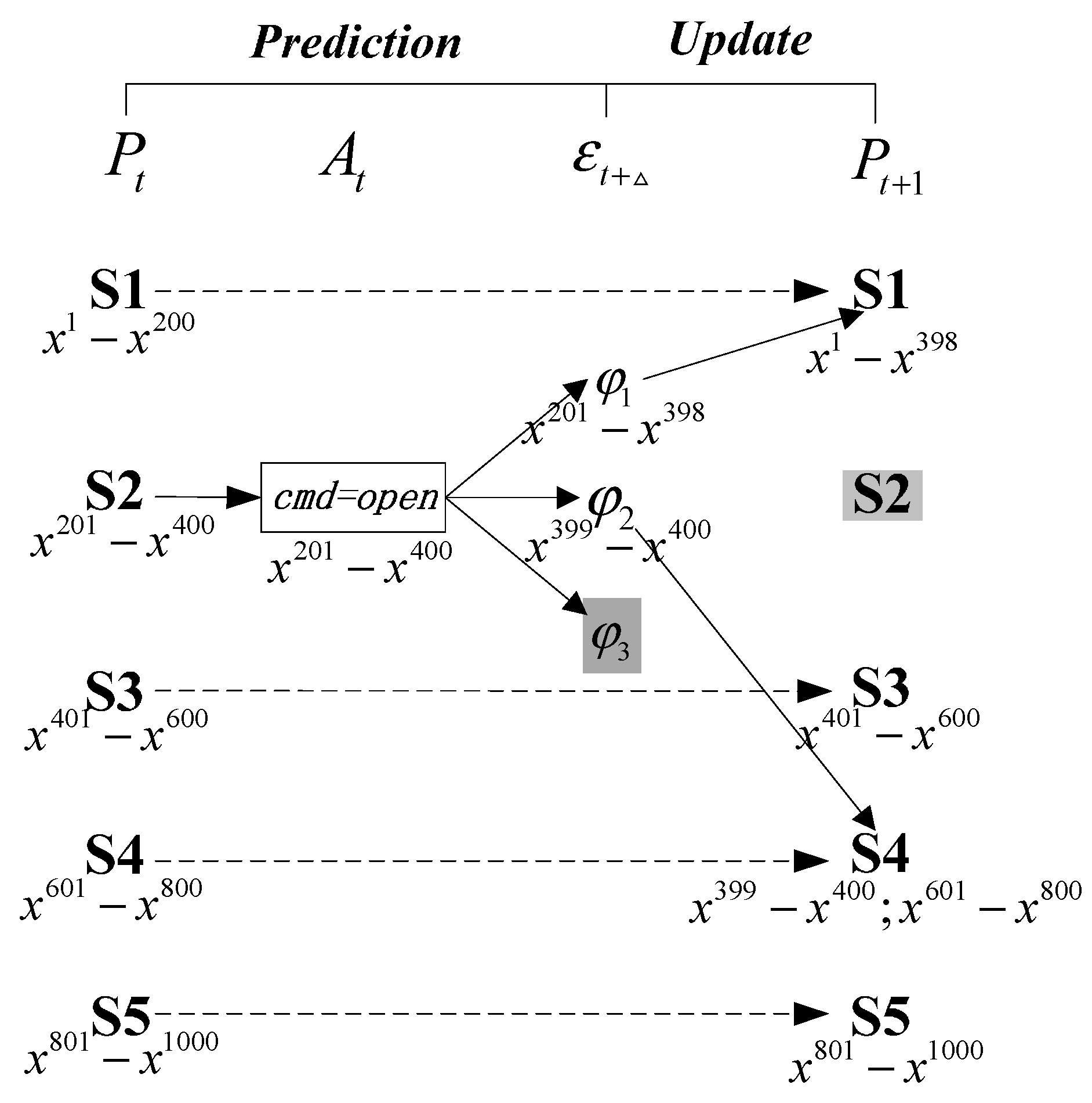
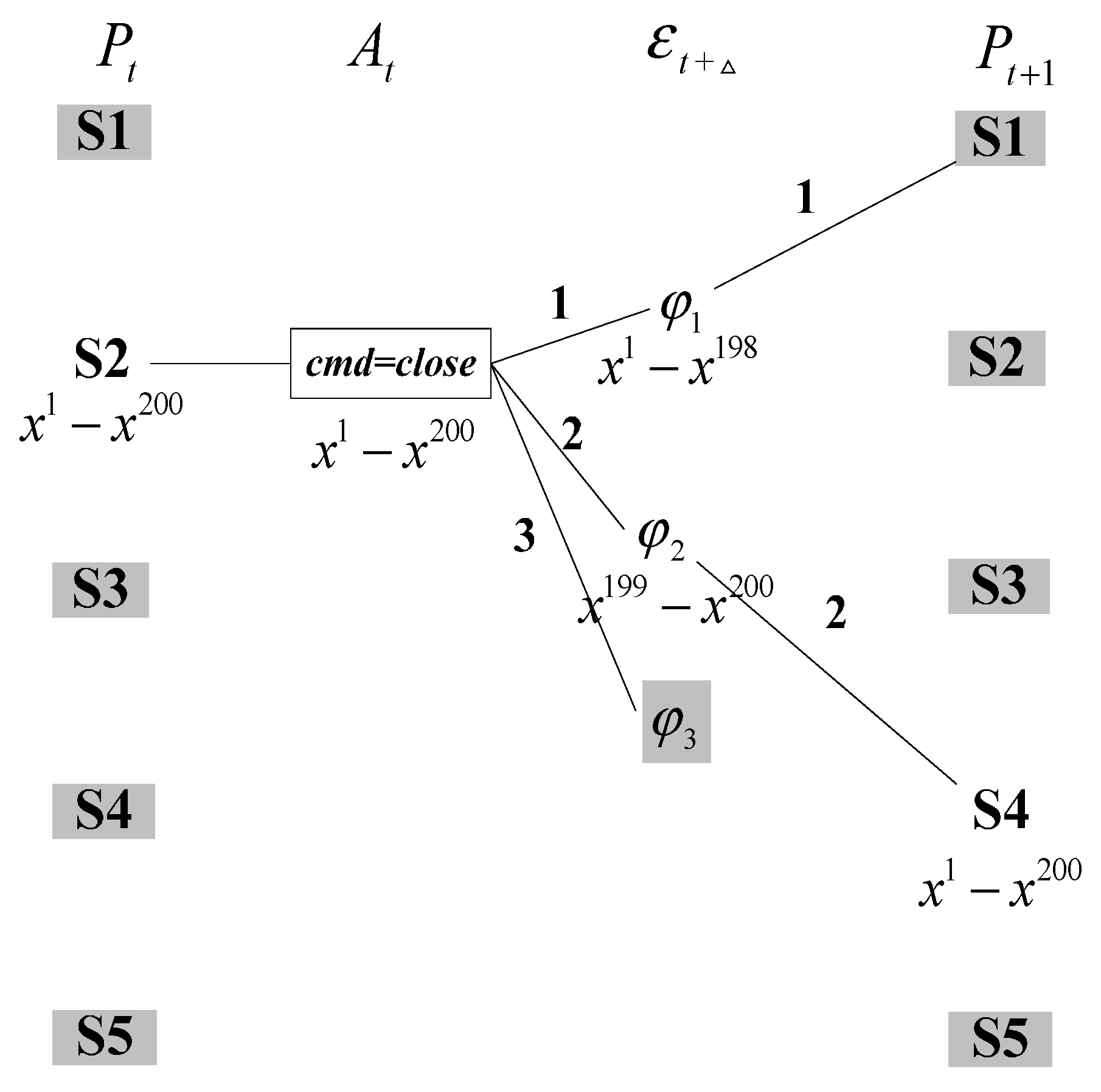
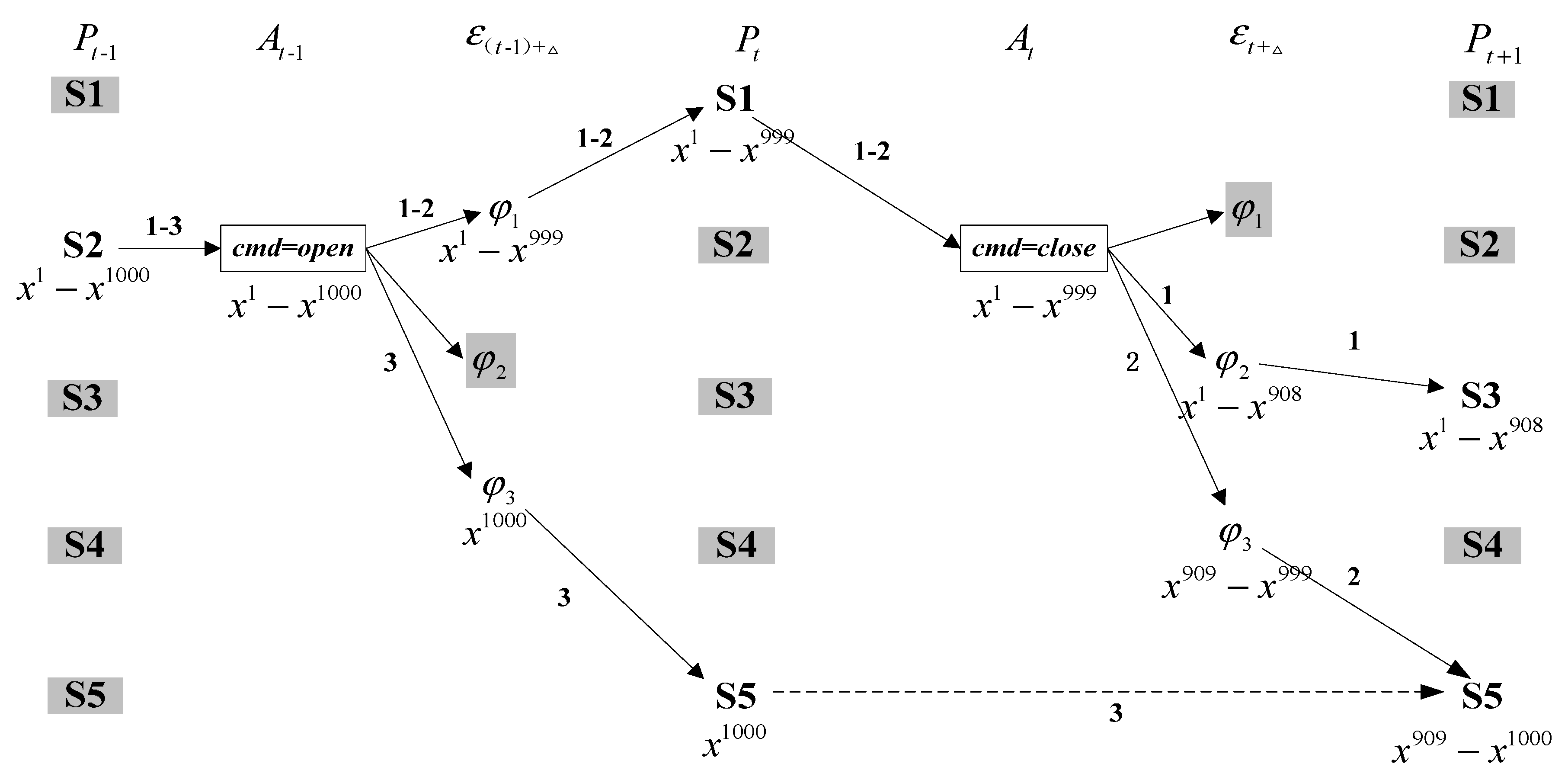
- Case 1: the effect can be assigned more than one particle according to the prior transition probability , and the observation is consistent with successor belief state (See path 2 in Figure 3).
- Case 2: the effect can also be distributed more than one particle, but the observation refutes the successor belief state (See path 1 in Figure 3).
- Case 3: the effect cannot be assigned one particle using the prior transition probability (See path 3 in Figure 3).
4.3.2. Complexity
| Best Case | Worst Case | |
|---|---|---|
| Roll forward process | ||
| Roll back process |
5. Experimental Results
| Source Mode | Transition Constraint | Possible Successor Modes | ||||
|---|---|---|---|---|---|---|
| M1 | M2 | M3 | M4 | M5 | ||
| M1 | sig_in < 97 | 0.989 | 0 | 0 | 0.01 | 0.001 |
| M1 | sig_in >= 97 sig_in <= 103 | 0.979 | 0 | 0 | 0.02 | 0.001 |
| M1 | sig_in > 103 | 0 | 0.959 | 0.02 | 0.02 | 0.001 |
| M2 | sig_in < 97 | 0.989 | 0 | 0 | 0.01 | 0.001 |
| M2 | sig_in >= 97 sig_in <= 103 | 0.979 | 0 | 0 | 0.02 | 0.001 |
| M2 | sig_in > 103 | 0 | 0.959 | 0.02 | 0.02 | 0.001 |
| M3 | - | 0 | 0 | 1 | 0 | 0 |
| M4 | - | 0 | 0 | 0 | 1 | 0 |
| M5 | - | 0 | 0 | 0 | 0 | 1 |
5.1. Basic Results
| Scenario | Average Time (ms) | Max Time (ms) |
|---|---|---|
| Nominal | 29.725 ± 0.634 | 85.46 |
| Single Fault | 67.873 ± 1.770 | 143.68 |
| Double Faults | 93.661 ± 5.198 | 328.65 |
| Three Faults | 103.759 ± 6.866 | 423.57 |
| Scenario | Expanded Nodes | Called Times of Consistency Function | ||
|---|---|---|---|---|
| Average Number | Max Number | Average Number | Max Number | |
| Nominal | 96.538 ± 1.6221 | 116 | 8.2000 ± 0.1384 | 18 |
| Single Fault | 103.455 ± 2.8798 | 151 | 14.4000 ± 0.6728 | 46 |
| Double Faults | 108.727 ± 3.0792 | 202 | 22.7000 ± 1.8675 | 110 |
| Three Faults | 115.545 ± 5.3045 | 273 | 24.5000 ± 2.1935 | 128 |
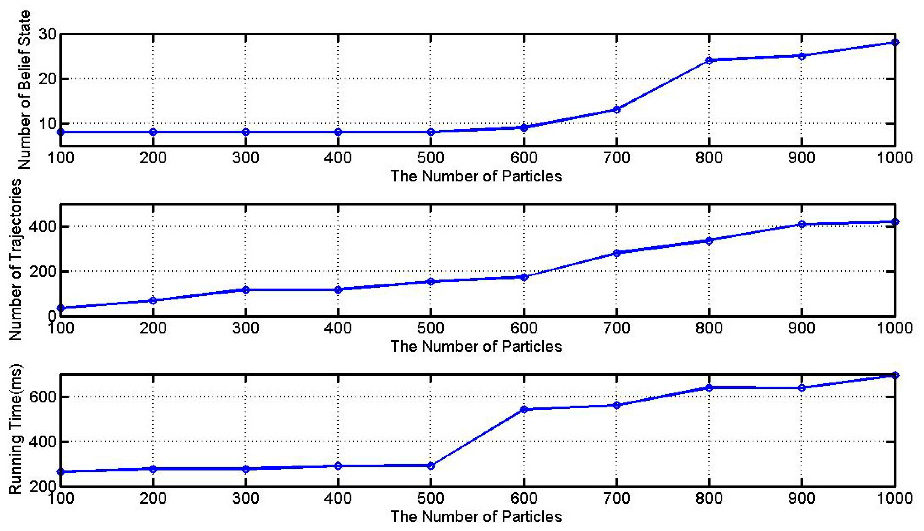
5.2. Number of Particles

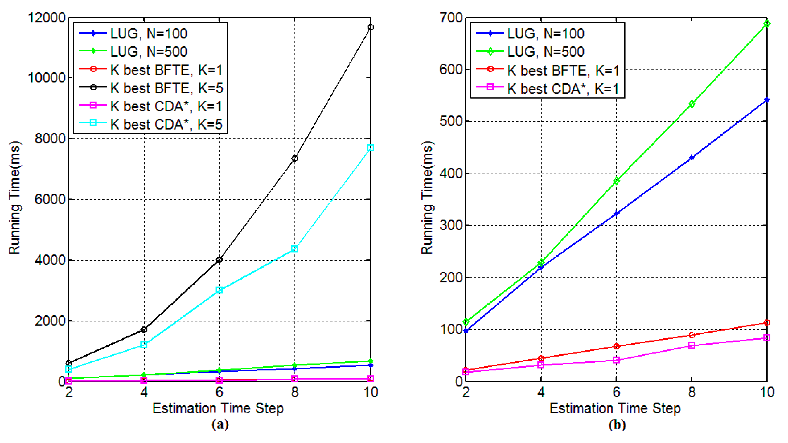
5.3. Comparison with Other Algorithms
| LUG | BFTE | CDA* | |||||||
|---|---|---|---|---|---|---|---|---|---|
| Time (ms) | Time (ms) | Time (ms) | |||||||
| 100 | 8 | 35 | 263.87 ± 0.21 | 1 | 1 | 51.97 ± 0.08 | 1 | 1 | 27.38 ± 0.03 |
| 200 | 8 | 67 | 276.70 ± 0.25 | 2 | 2 | 156.89 ± 0.12 | 2 | 2 | 82.15 ± 0.05 |
| 300 | 8 | 117 | 277.38 ± 0.32 | 3 | 3 | 489.86 ± 0.43 | 3 | 3 | 194.76 ± 0.45 |
| 400 | 8 | 117 | 289.23 ± 0.47 | 4 | 3 | 809.56 ± 0.54 | 4 | 3 | 375.23 ± 0.49 |
| 500 | 8 | 152 | 292.08 ± 0.63 | 5 | 3 | 1352.88 ± 0.61 | 5 | 3 | 587.18 ± 0.58 |
| 600 | 9 | 174 | 541.17 ± 0.67 | 6 | 3 | 2307.51 ± 0.65 | 6 | 3 | 961.42 ± 0.69 |
| 700 | 13 | 280 | 559.83 ± 0.71 | 7 | 3 | 3573.87 ± 0.73 | 7 | 3 | 1276.36 ± 0.76 |
| 800 | 24 | 337 | 640.24 ± 0.77 | 8 | 3 | 4922.32 ± 0.82 | 8 | 3 | 2058.53 ± 0.71 |
| 900 | 25 | 408 | 638.71 ± 0.81 | 9 | 3 | 6214.18 ± 1.03 | 9 | 3 | 3468.74 ± 0.92 |
| 1000 | 28 | 419 | 692.72 ± 0.85 | 10 | 4 | 8446.02 ± 1.15 | 10 | 4 | 4185.69 ± 0.97 |
6. Conclusions
Acknowledgments
Author Contributions
Conflicts of Interest
References
- Roychoudhury, I.; Biswas, G.; Koutsoukos, X. Designing distributed diagnosers for complex continuous systems. IEEE Trans. Autom. Sci. 2009, 6, 277–290. [Google Scholar] [CrossRef]
- Yi, C.; Lin, J.; Zhang, W.; Ding, J. Faults Diagnostics of Railway Axle Bearings Based on IMF’s Confidence Index Algorithm for Ensemble EMD. Sensors 2015, 15, 10991–11011. [Google Scholar] [CrossRef] [PubMed]
- Lv, Y.; Zhu, Q.; Yuan, R. Fault Diagnosis of Rolling Bearing Based on Fast Nonlocal Means and Envelop Spectrum. Sensors 2015, 15, 1182–1198. [Google Scholar] [CrossRef] [PubMed]
- Ranjbar, A.M.; Shirani, A.R.; Fathi, A.F. A new approach for fault location problem on power lines. IEEE Trans. Power Deliv. 1992, 7, 146–151. [Google Scholar] [CrossRef]
- Gertler, J. Fault Detection and Diagnosis in Engineering Systems; CRC Press: New York, NY, USA, 1998. [Google Scholar]
- Jiang, T.; Khorasani, K.; Tafazoli, S. Parameter estimation-based fault detection, isolation and recovery for nonlinear satellite models. IEEE Trans. Control Syst. Technol. 2008, 16, 799–808. [Google Scholar] [CrossRef]
- Dearden, R.; Willeke, T.; Simmons, R.; Verma, V.; Hutter, F.; Thrun, S. Real-time fault detection and situational awareness for rovers: Report on the mars technology program task. In Proceedings of the IEEE Aerospace Conference, Moffett Field, CA, USA, 6–13 March 2004; pp. 826–840.
- Zaytoon, J.; Lafortune, S. Overview of fault diagnosis methods for Discrete Event Systems. Annu. Rev. Control. 2013, 37, 308–320. [Google Scholar] [CrossRef]
- Torta, G.; Torasso, P. An on-line approach to the computation and presentation of preferred diagnoses for dynamic systems. AI Commun. 2007, 20, 93–116. [Google Scholar]
- Cerutti, S.; Lamperti, G.; Scaroni, M.; Zanella, M.; Zanni, D. A diagnostic environment for automaton networks. Softw. Pract. Exp. 2007, 37, 365–415. [Google Scholar] [CrossRef]
- Pencolé, Y.; Cordier, M.O.; Rozé, L. A decentralized model-based diagnostic tool for complex systems. Int. J. Artif. Intell. Tools 2002, 11, 327–346. [Google Scholar] [CrossRef]
- Pencolé, Y.; Cordier, M.O. A formal framework for the decentralised diagnosis of large scale discrete event systems and its application to telecommunication networks. Artif. Intell. 2005, 164, 121–170. [Google Scholar] [CrossRef]
- Cordier, M.O.; Dague, P.; Lévy, F.; Montmain, J.; Staroswiecki, M.; Travé-Massuyès, L. Conflicts versus analytical redundancy relations: A comparative analysis of the model based diagnosis approach from the artificial intelligence and automatic control perspectives. IEEE Trans. Syst. Man Cybern. Part B Cybern. 2004, 34, 2163–2177. [Google Scholar] [CrossRef]
- Bregon, A.; Biswas, G.; Pulido, B.; Alonso-Gonzalez, C.; Khorasgani, H. A Common Framework for Compilation Techniques Applied to Diagnosis of Linear Dynamic Systems. IEEE Trans. Syst. Man Cybern. Syst. 2014, 44, 863–876. [Google Scholar] [CrossRef]
- Travé-Massuyès, L. Bridging control and artificial intelligence theories for diagnosis: A survey. Eng. Appl. Artif. Intell. 2014, 27, 1–16. [Google Scholar] [CrossRef]
- Sampath, M.; Sengupta, R.; Lafortune, S.; Sinnamohideen, K.; Teneketzis, D.C. Failure diagnosis using discrete-event models. IEEE Trans. Control Syst. Technol. 1996, 4, 105–124. [Google Scholar] [CrossRef]
- Sampath, M.; Sengupta, R.; Lafortune, S.; Sinnamohideen, K.; Teneketzis, D. Diagnosability of discrete-event systems. IEEE Trans. Autom. Control 1995, 40, 1555–1575. [Google Scholar] [CrossRef]
- Schumann, A.; Pencolé, Y.; Thiébaux, S. A Spectrum of Symbolic On-Line Diagnosis Approaches. In Proceedings of the 18th International Workshop on Principles of Diagnosis, Nashville, TN, USA, 29–31 May 2007; pp. 194–199.
- Baroni, P.; Lamperti, G.; Pogliano, P.; Zanella, M. Diagnosis of large active systems. Artif. Intell. 1999, 110, 135–183. [Google Scholar] [CrossRef]
- Mohammadi-Idghamishi, A.; Hashtrudi-Zad, S. Hierarchical fault diagnosis: Application to an ozone plant. IEEE Trans. Syst. Man Cybern. Part C Appl. Rev. 2007, 37, 1040–1047. [Google Scholar] [CrossRef]
- Williams, B.C.; Nayak, P.P. A model-based approach to reactive self-configuring systems. In Proceedings of the National Conference on Artificial Intelligence, Portland, OR, USA, 4–8 August 1996; pp. 971–978.
- Kurien, J.; Nayak, P.P. Back to the future for consistency-based trajectory tracking. In Proceedings of the National Conference on Artificial Intelligence, Austin, TX, USA, 30 July–3 August 2000; pp. 370–377.
- Martin, O.B.; Williams, B.C.; Ingham, M.D. Diagnosis as approximate belief state enumeration for probabilistic concurrent constraint automata. In Proceedings of the National Conference on Artificial Intelligence, Pittsburgh, PA, USA, 9–13 July 2005; pp. 321–326.
- Williams, B.C.; Ragno, R.J. Conflict-directed A* and its role in model-based embedded systems. Discret. Appl. Math. 2007, 155, 1562–1595. [Google Scholar] [CrossRef]
- Bryce, D.; Kambhampati, S.; Smith, D.E. Planning graph heuristics for belief space search. J. Artif. Intell. Res. 2006, 26, 35–99. [Google Scholar] [CrossRef]
- Wang, M.; Dearden, R. Detecting and learning unknown fault states in hybrid diagnosis. In Proceedings of the 20th International Workshop on Principles of Diagnosis, Stockholm, Sweden, 14–17 June 2009; pp. 19–26.
- Reiter, R. A theory of diagnosis from first principles. Artif. Int. 1987, 32, 57–95. [Google Scholar] [CrossRef]
- Verma, I.; Thrun, S.; Simmons, R. Variable resolution particle filter. In Proceedings of the International Joint Conference of Artificial Intelligence, Acapulco, Mexico, 9–15 August 2003; pp. 976–981.
- Bryce, D.; Cushing, W.; Kambhampati, S. State agnostic planning graphs: Deterministic, non-deterministic, and probabilistic planning. Artif. Int. 2011, 175, 848–889. [Google Scholar] [CrossRef]
- Bryce, D. Scalable Planning under Uncertainty. Ph.D. Thesis, Arizona State University, Tempe, AZ, USA, 2007. [Google Scholar]
- Haslum, P.; Grastien, A. Diagnosis as planning: Two case studies. In Proceedings of the International Scheduling and Planning Applications workshop, Freiburg, Germany, 11–16 June 2011.
- Gilks, W.R. Markov Chain Monte Carlo; John Wiley & Sons, Ltd.: Hoboken, NJ, USA, 2005. [Google Scholar]
- Russell, S.; Norvig, P. Artificial Intelligence: A Modern Approach, 3rd ed.; Prentice Hall: Upper Saddle River, NJ, USA, 2010. [Google Scholar]
- Struss, P.; Dressler, O. “Physical Negation” Integrating Fault Models into the General Diagnostic Engine. In Proceedings of the International Joint Conference of Artificial Intelligence, Detroit, MI, USA, 20–25 August 1989.
- Blackmore, L.; Funiak, S.; Williams, B.C. A combined stochastic and greedy hybrid estimation capability for concurrent hybrid models with autonomous mode transitions. Robot. Auton. Syst. 2008, 56, 105–129. [Google Scholar] [CrossRef]
© 2015 by the authors; licensee MDPI, Basel, Switzerland. This article is an open access article distributed under the terms and conditions of the Creative Commons Attribution license (http://creativecommons.org/licenses/by/4.0/).
Share and Cite
Zhou, G.; Feng, W.; Zhao, Q.; Zhao, H. State Tracking and Fault Diagnosis for Dynamic Systems Using Labeled Uncertainty Graph. Sensors 2015, 15, 28031-28051. https://doi.org/10.3390/s151128031
Zhou G, Feng W, Zhao Q, Zhao H. State Tracking and Fault Diagnosis for Dynamic Systems Using Labeled Uncertainty Graph. Sensors. 2015; 15(11):28031-28051. https://doi.org/10.3390/s151128031
Chicago/Turabian StyleZhou, Gan, Wenquan Feng, Qi Zhao, and Hongbo Zhao. 2015. "State Tracking and Fault Diagnosis for Dynamic Systems Using Labeled Uncertainty Graph" Sensors 15, no. 11: 28031-28051. https://doi.org/10.3390/s151128031
APA StyleZhou, G., Feng, W., Zhao, Q., & Zhao, H. (2015). State Tracking and Fault Diagnosis for Dynamic Systems Using Labeled Uncertainty Graph. Sensors, 15(11), 28031-28051. https://doi.org/10.3390/s151128031