
Dynamic Performance Comparison of Two Kalman Filters for Rate Signal Direct Modeling and Differencing Modeling for Combining a MEMS Gyroscope Array to Improve Accuracy


Abstract
:
1. Introduction
2. Methodology Comparison of the Virtual Gyroscope System Model
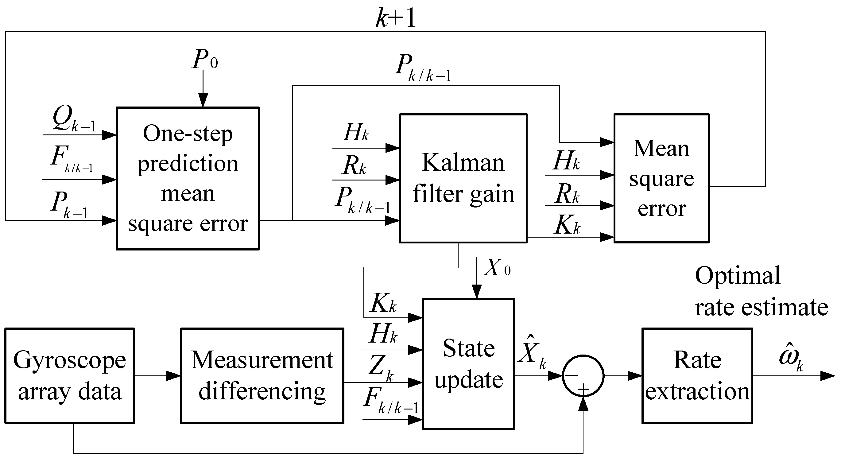
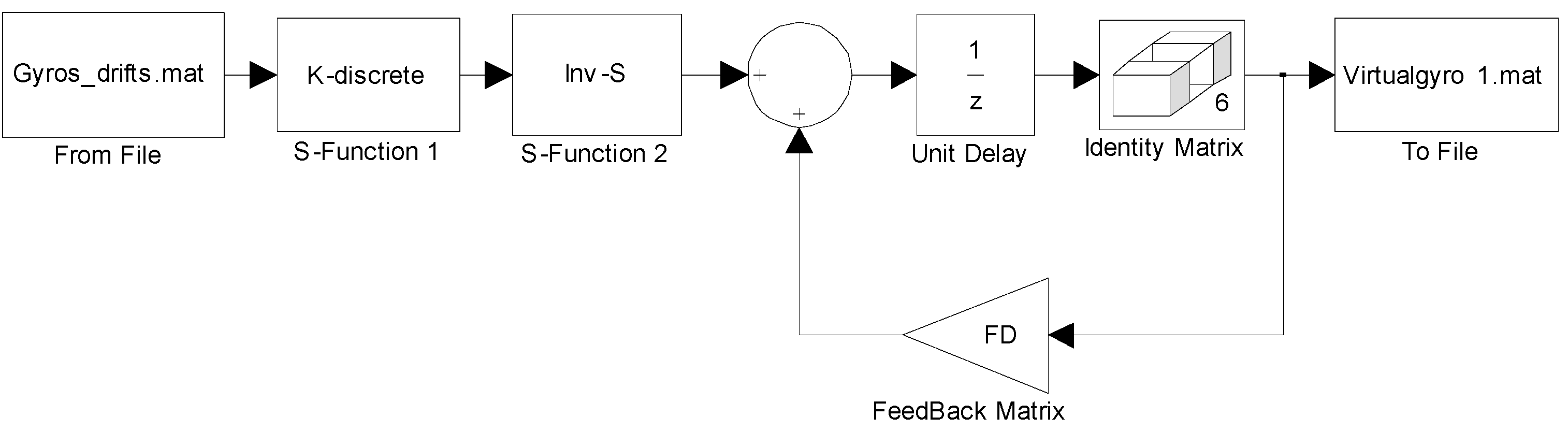
2.1. Direct Estimated Model for Virtual Gyroscope System
2.2. Differencing Estimated Model for the Virtual Gyroscope System

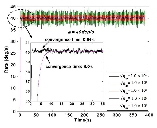
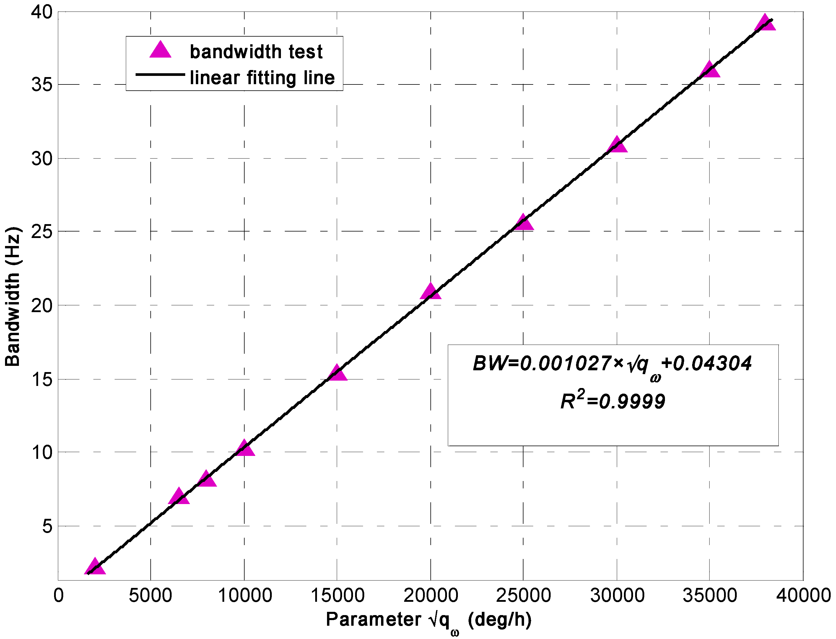
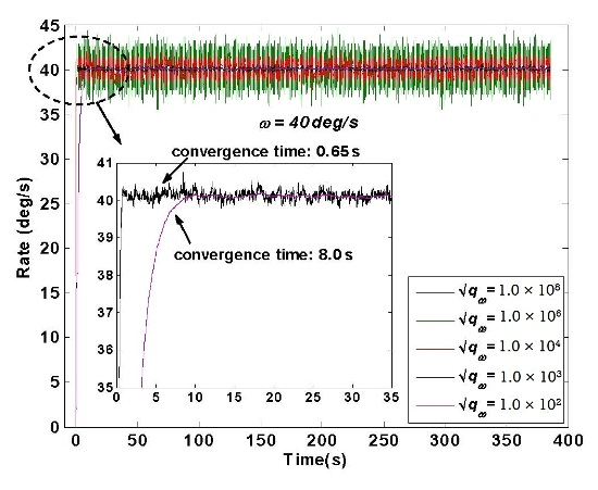
3. Bandwidth Analysis of the Two KF Models

| Coefficient | P1 | P2 | SSE | RMSE | R2 |
|---|---|---|---|---|---|
| Value | 0.001027 | 0.04304 | 0.1961 | 0.1566 | 0.9999 |
| Bound | (0.001018, 0.001037) | (–0.1704, 0.2565) |
4. Dynamic Simulation Comparison of Two KF Models
4.1. Constant Rate Simulation Result

| Virtual Gyroscope KF Model | (°/h) | Mean of Estimated Rate Signal (°/s) | STD of Estimated Error (1σ, °/s) |
|---|---|---|---|
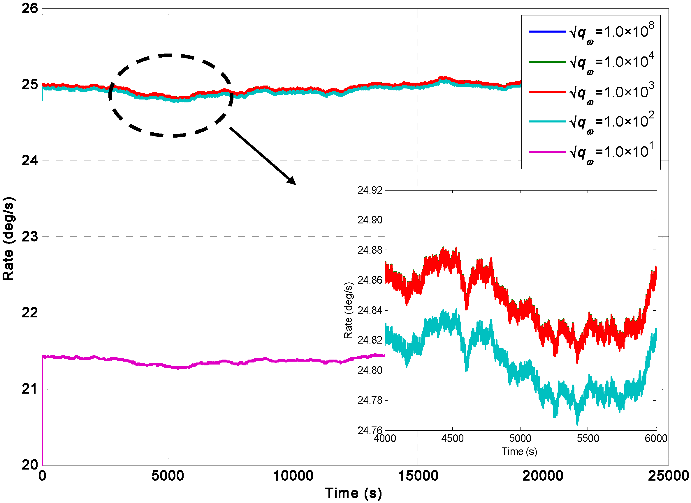
| Direct Estimated Model | 1.0 × 10⁸ | 24.9576 | 0.0594 |
| 1.0 × 10⁴ | 24.9576 | 0.0592 | |
| 1.0 × 10³ | 24.9572 | 0.0590 | |
| 1.0 × 10² | 24.9161 | 0.0591 | |
| 10 | 21.3921 | 0.0613 | |
| Differencing Estimated Model | — | 24.9576 | 0.0613 |
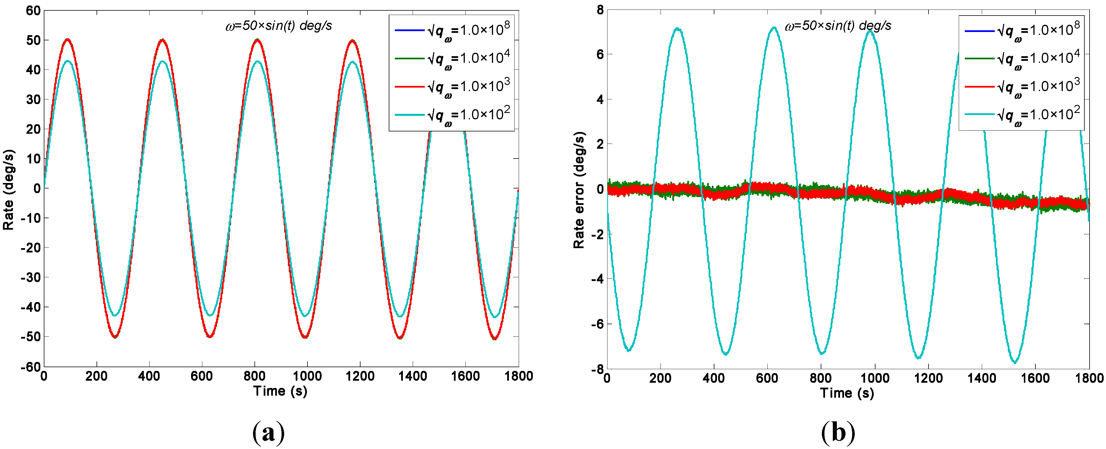
4.2. Sinusoidal Rate Simulation Result

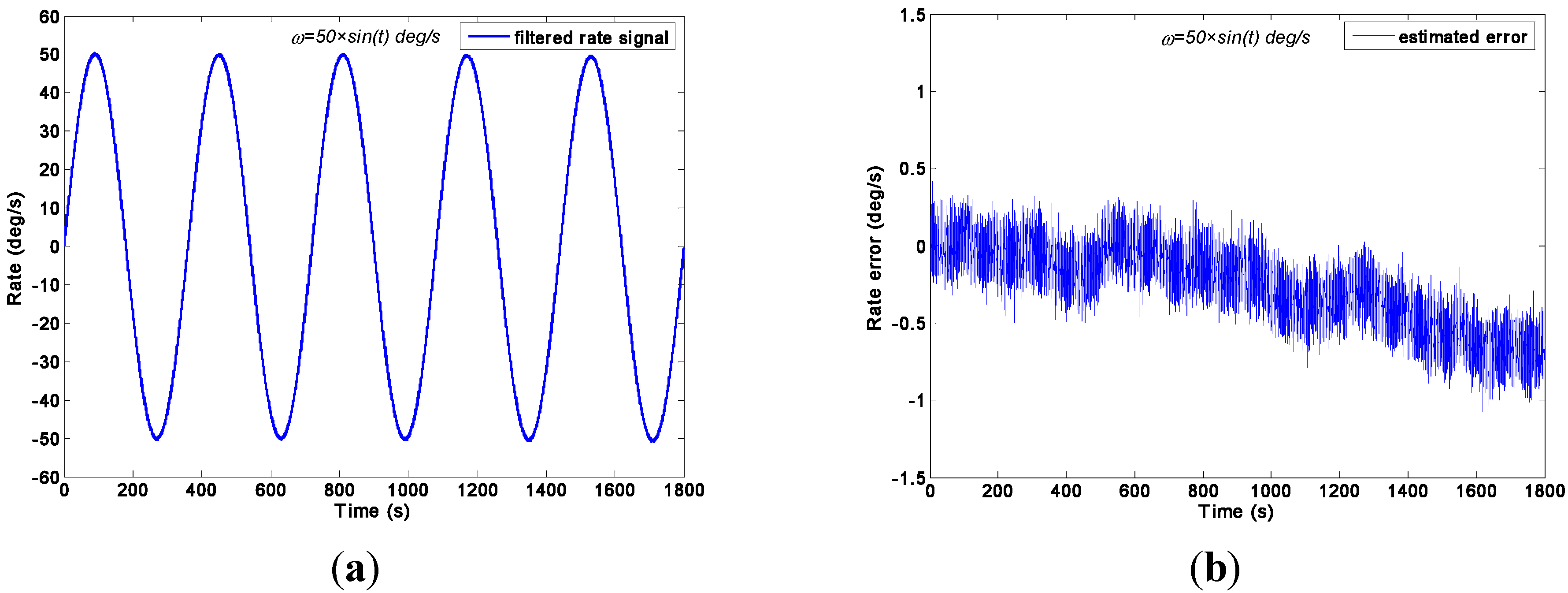
| Virtual Gyroscope KF Model | (°/h) | Amplitude of Rate Signal (°/s) | STD of Estimated Error (1σ, °/s) |
|---|---|---|---|
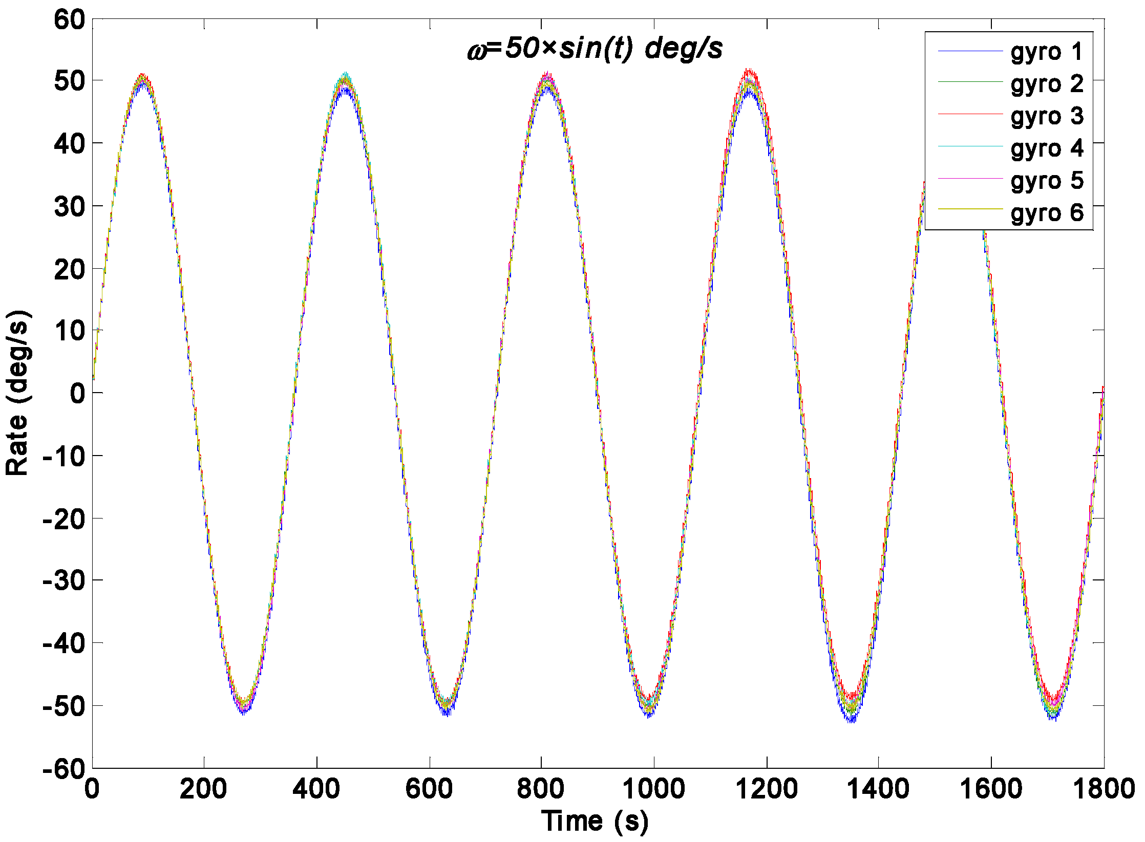
| Direct Estimated Model | 1.0 × 10⁸ | 50.2677 | 0.2506 |
| 1.0 × 10⁴ | 50.2668 | 0.2505 | |
| 1.0 × 10³ | 50.1195 | 0.2480 | |
| 1.0 × 10² | 42.9318 | 5.0860 | |
| Differencing Estimated Model | — | 50.2677 | 0.2506 |
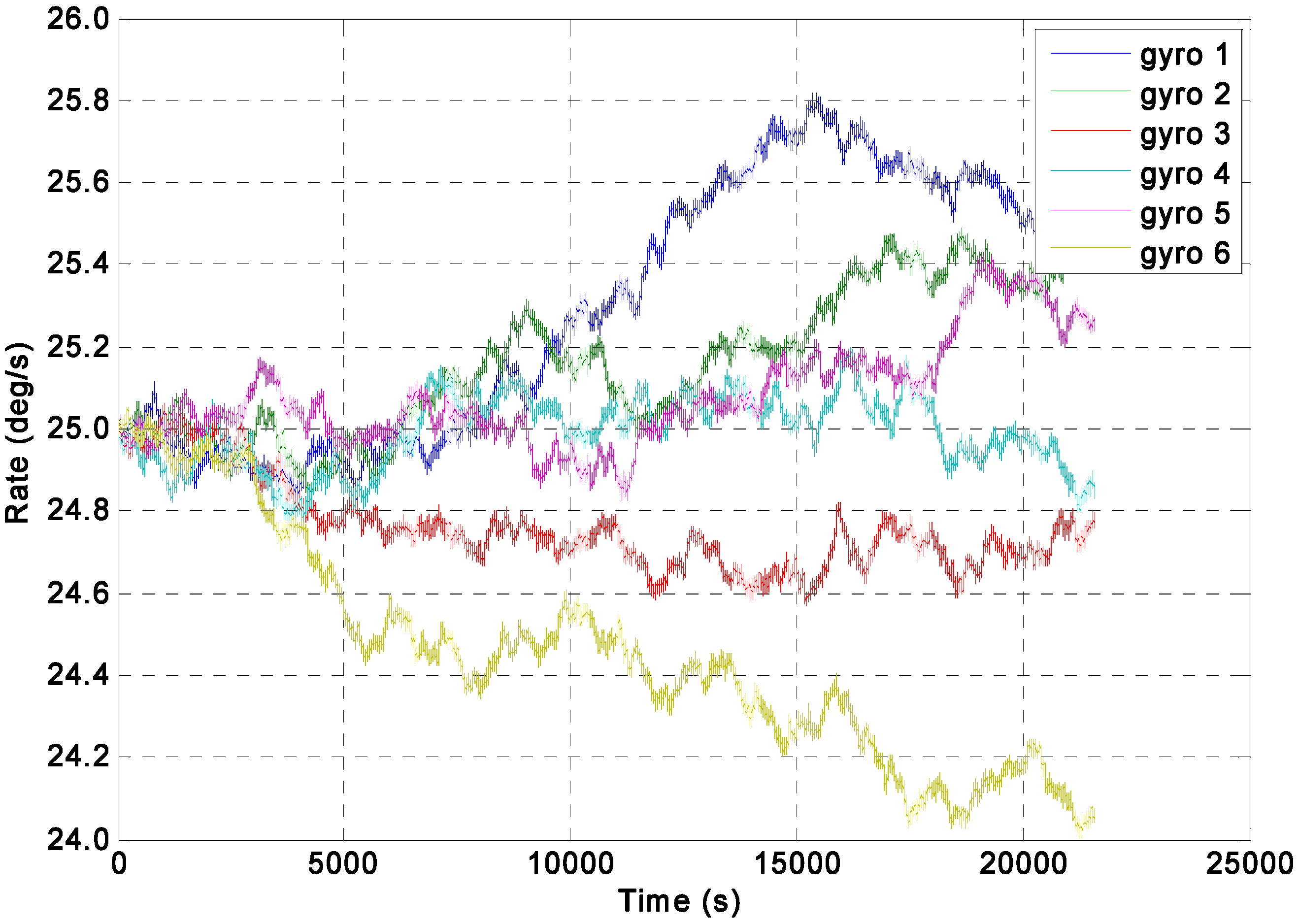
| Original Individual Gyroscope | — | 51.1120 | 0.5072 |
5. Dynamic Experiment Comparison and Discussion

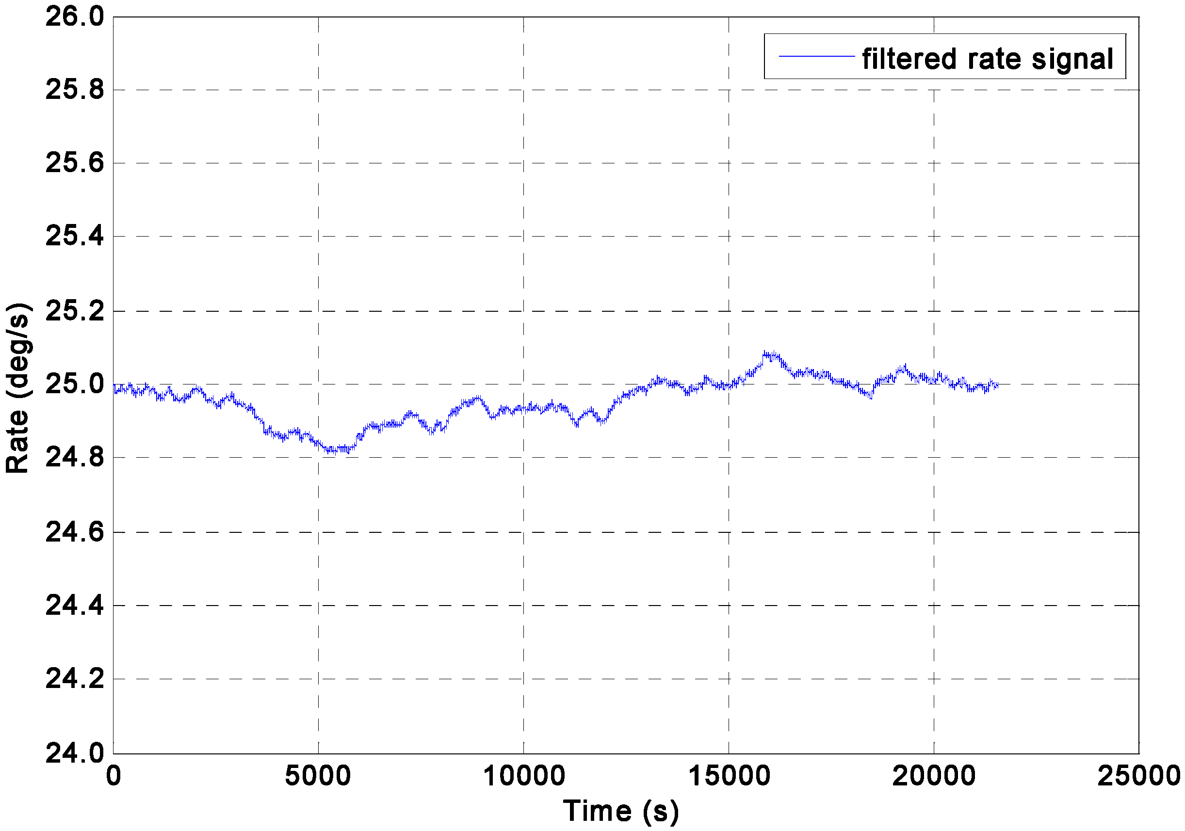
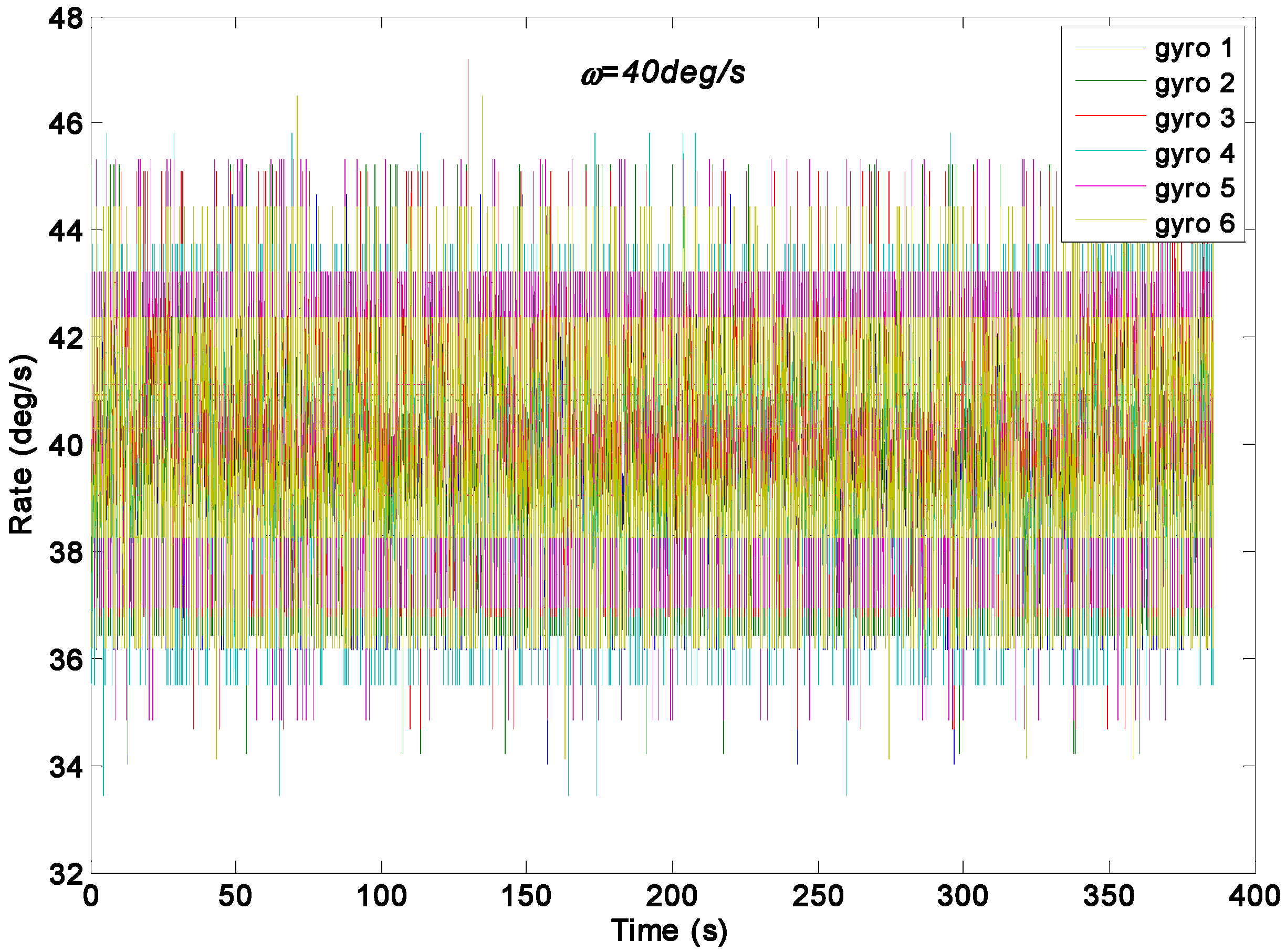
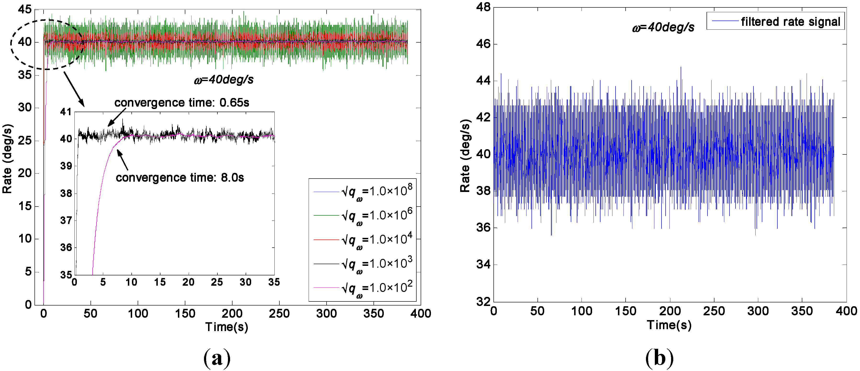
5.1. Constant Rate Signal Test Result


| Virtual gyroscope KF model | (°/h) | Mean of Estimated Signal (°/s) | STD of Rate Error (1σ, °/s) |
|---|---|---|---|
| Direct Estimated Model | 1.0 × 10⁸ | 40.1457 | 0.5960 |
| 1.0 × 10⁶ | 40.1457 | 0.5857 | |
| 1.0 × 10⁴ | 40.1445 | 0.5235 | |
| 1.0 × 10³ | 40.1301 | 0.1203 | |
| 1.0 × 10² | 39.9752 | 0.0832 | |
| Differencing Estimated Model | — | 40.1457 | 0.5974 |
| Original Individual Gyroscope | — | 40.2457 | 1.4558 |
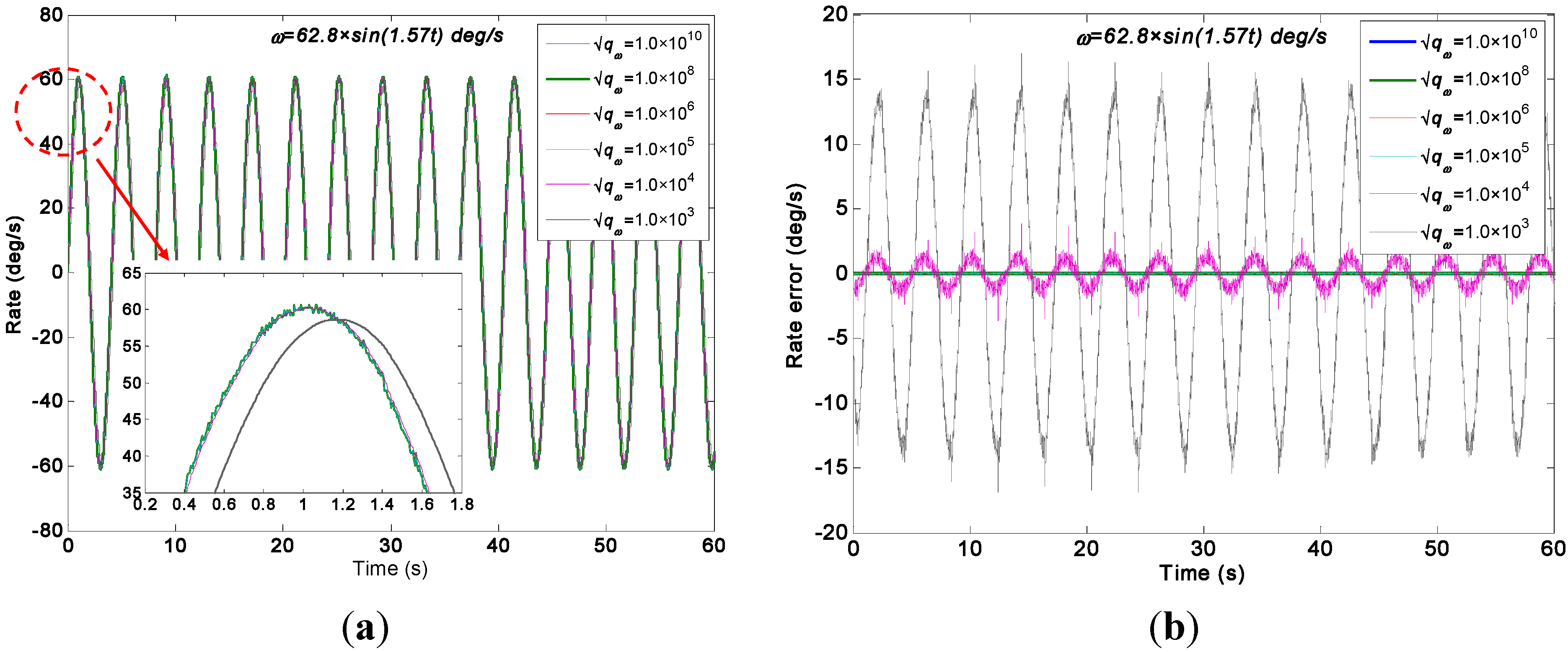
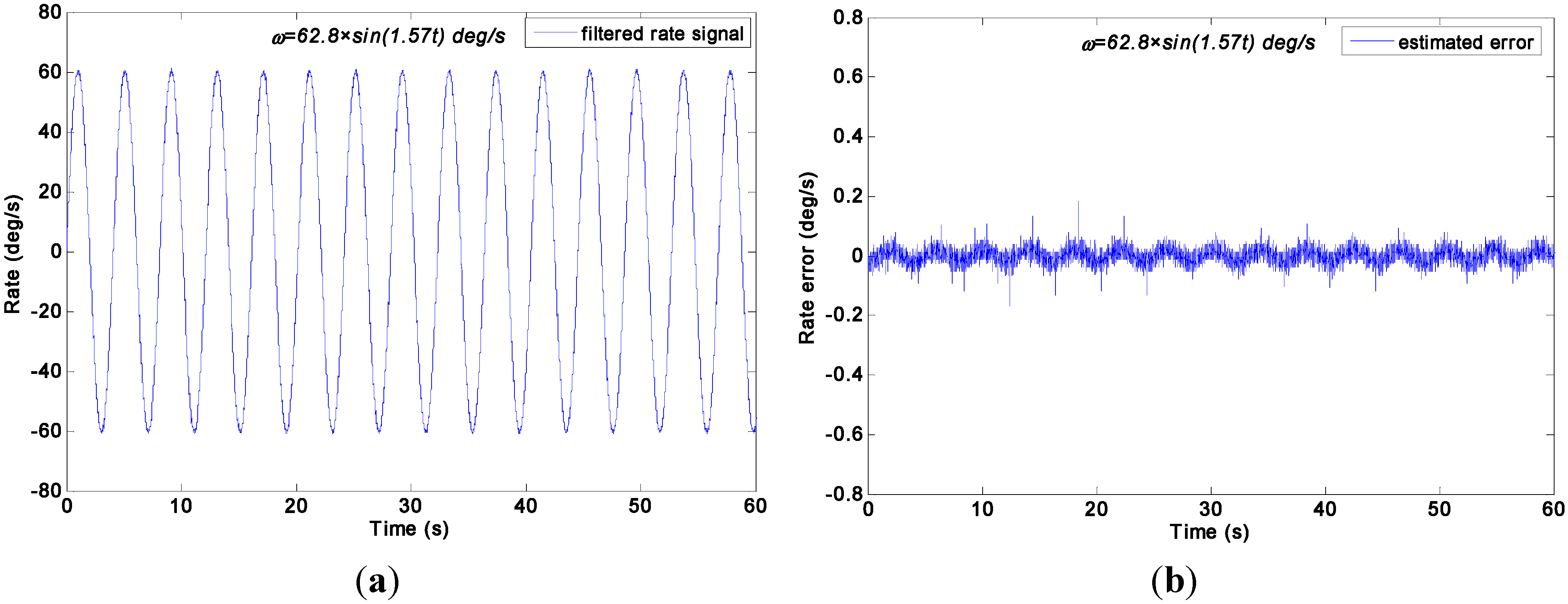
5.2. Swing Rate Signal Test Result
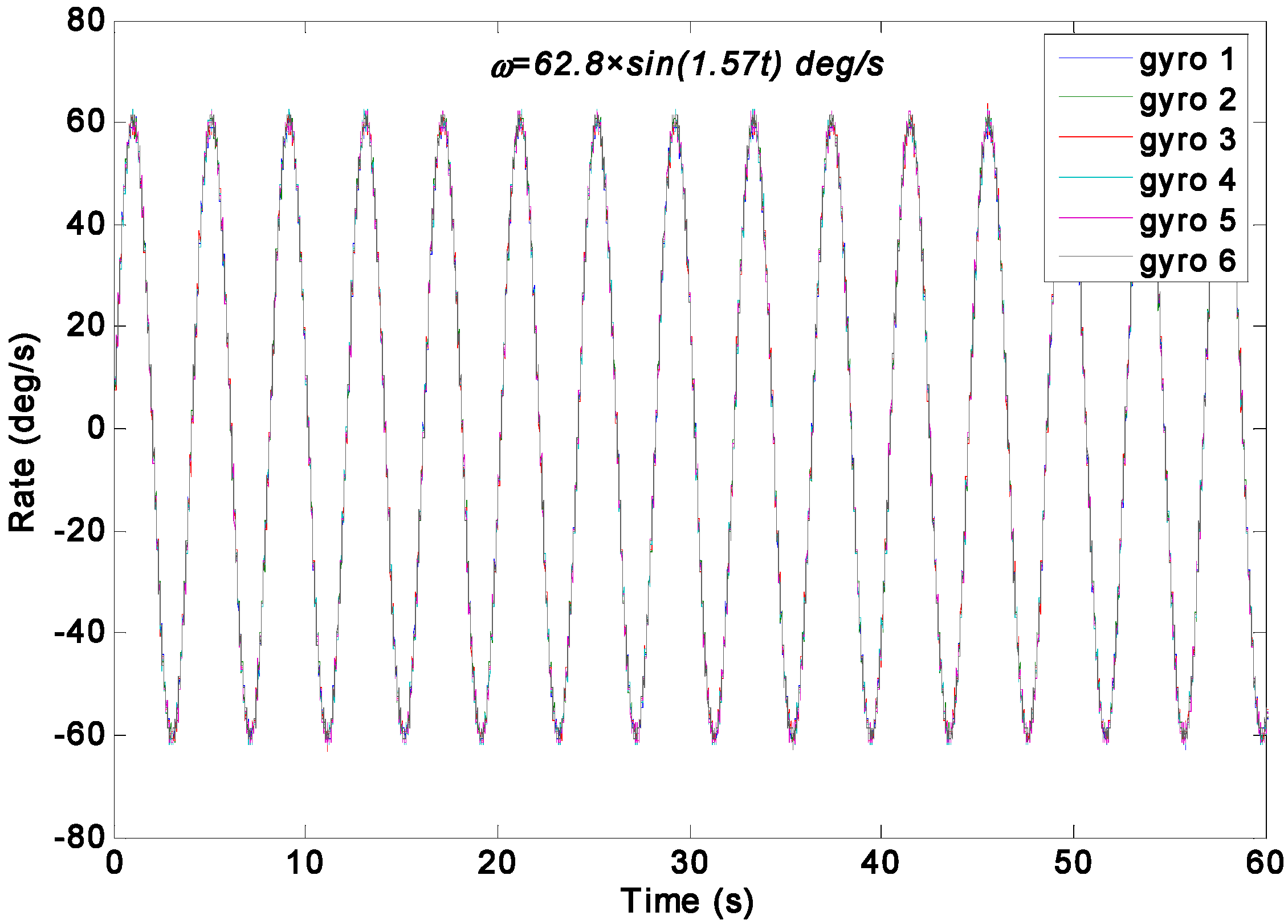


| Virtual Gyroscope Model | (°/h) | Amplitude of Rate Signal (°/s) | STD of Rate Error (1σ, °/s) |
|---|---|---|---|
| Direct Estimated Model | 1.0 × 10¹⁰ | 61.2876 | 0.6195 |
| 1.0 × 10⁸ | 61.2876 | 0.6011 | |
| 1.0 × 10⁶ | 61.2876 | 0.5428 | |
| 1.0 × 10⁵ | 61.2554 | 0.5202 | |
| 1.0 × 10⁴ | 60.6423 | 0.9140 | |
| 1.0 × 10³ | 58.7606 | 9.7288 | |
| Differencing Estimated Model | — | 61.2876 | 0.6079 |
| Original Individual Gyroscope | — | 62.6428 | 1.6231 |
6. Conclusions
Acknowledgments
Author Contributions
Conflicts of Interest
References
- Sonmezoglu, S.; Alper, S.E.; Akin, T. An automatically mode-matched MEMS gyroscope with wide and tunable bandwidth. J. Microelectromech. Syst. 2014, 23, 284–297. [Google Scholar] [CrossRef]
- Ahn, C.H.; Ng, E.J.; Hong, V.A.; Yang, Y.; Lee, B.J.; Flader, I.; Kenny, T.W. Mode-matching of wineglass mode disk resonator gyroscope in (100) single crystal silicon. J. Microelectromech. Syst. 2015, 24, 343–350. [Google Scholar] [CrossRef]
- Tatar, E.; Mukherjee, T.; Fedder, G.K. Tuning of nonlinearities and quality factor in a mode-matched gyroscope. In Proceedings of the IEEE 27th International Conference on Micro Electro Mechanical Systems, San Francisco, CA, USA, 26–30 January 2014; pp. 801–804.
- Liu, K.; Zhang, W.P.; Chen, W.Y.; Li, K.; Dai, F.Y.; Cui, F.; Wu, X.S.; Ma, G.Y.; Xiao, Q.J. The development of micro-gyroscope technology. J. Micromech. Microeng. 2009, 19, 157–185. [Google Scholar] [CrossRef]
- Bayard, D.S.; Ploen, S.R. High Accuracy Inertial Sensors from Inexpensive Components. U.S. Patent No. 20030187623A1, 2 October 2003. [Google Scholar]
- Chang, H.L.; Xue, L.; Qin, W.; Yuan, G.M.; Yuan, W.Z. An integrated MEMS gyroscope array with higher accuracy output. Sensors 2008, 8, 2886–2899. [Google Scholar] [CrossRef]
- Xue, L.; Jiang, C.Y.; Chang, H.L.; Yang, Y.; Qin, W.; Yuan, W.Z. A novel Kalman filter for combining outputs of MEMS gyroscope array. Measurement 2012, 45, 745–754. [Google Scholar] [CrossRef]
- Chang, H.L.; Xue, L.; Jiang, C.Y.; Kraft, M.; Yuan, W.Z. Combining numerous uncorrelated MEMS gyroscopes for accuracy improvement based on an optimal Kalman filter. IEEE Trans. Instrum. Meas. 2012, 61, 3084–3093. [Google Scholar] [CrossRef]
- Xue, L.; Jiang, C.Y.; Wang, L.X.; Liu, J.Y.; Yuan, W.Z. Noise reduction of MEMS gyroscope based on direct modeling for an angular rate signal. Micromachines 2015, 6, 266–280. [Google Scholar] [CrossRef]
- Colomina, I.; Giménez, M.; Rosales, J.J.; Wis, M.; Gomez, A.; Miguelsanz, P. Redundant IMUs for precise trajectory determination. In Proceedings of the 20th International Society for Photogrammetry and Remote Sensing Congress, Istanbul, Turkey, 12–23 July 2004; pp. 1–7.
- Waegli, A.; Skaloud, J.; Guerrier, S.; Parés, M.E.; Colomina, I. Noise reduction and estimation in multiple micro-electro-mechanical inertial systems. Meas. Sci. Technol. 2010, 21. [Google Scholar] [CrossRef]
- Xue, L.; Wang, L.X.; Xiong, T.; Jiang, C.Y.; Yuan, W.Z. Analysis of dynamic performance of a Kalman filter for combining multiple MEMS gyroscopes. Micromachines 2014, 5, 1034–1050. [Google Scholar] [CrossRef]
- Chang, H.L.; Zhang, P.; Hu, M.; Yuan, W.Z. On improving the accuracy of the micromachined gyroscopes based on the multi-sensor fusion. In Proceedings of the International Conference on Integration and Commercialization of Micro and Nanosystems, Sanya, China, 10–13 January 2007; pp. 213–217.
- Jiang, C.; Xue, L.; Chang, H.; Yuan, G.; Yuan, W. Signal processing of MEMS gyroscope arrays to improve accuracy using a 1st order Markov for rate signal modeling. Sensors 2012, 12, 1720–1737. [Google Scholar] [CrossRef] [PubMed]
- Lam, Q.M.; Hunt, T.; Sanneman, P.; Underwood, S. Analysis and design of a fifteen state stellar inertial attitude determination system. In Proceedings of the AIAA Guidance, Navigation, and Control Conference and Exhibit, Austin, TX, USA, 11–14 August 2003; p. 5483.
- Stearns, H.; Tomizuka, M. Multiple model adaptive estimation of satellite attitude using MEMS gyros. In Proceedings of the American Control Conference, San Francisco, CA, USA, 29 June–1 July 2011; pp. 3490–3495.
- El-Sheimy, N.; Hou, H.Y.; Niu, X.J. Analysis and modeling of inertial sensors using Allan variance. IEEE Trans. Instrum. Meas. 2008, 57, 140–149. [Google Scholar] [CrossRef]
- Vaccaro, R.J.; Zaki, A.S. Statistical modeling of rate gyros. IEEE Trans. Instrum. Meas. 2012, 61, 673–684. [Google Scholar] [CrossRef]
- Guerrier, S.; Skaloud, J.; Stebler, Y.; Victoria-Feser, M.-P. Wavelet variance based estimation for composite stochastic processes. J. Am. Stat. Assoc. 2013, 108, 1021–1030. [Google Scholar] [CrossRef] [PubMed]
- Grewal, M.S.; Andrews, A.P. Kalman Filtering Theory and Practice Using Matlab, 2nd ed.; John Wiley & Sons: New York, NY, USA, 2001; pp. 119–121. [Google Scholar]
- Analog Devices, ADXRS300. Available online: http://www.analog.com/static/imported-files/data_sheets/ADXRS300.pdf (accessed on 10 March 2015).
© 2015 by the authors; licensee MDPI, Basel, Switzerland. This article is an open access article distributed under the terms and conditions of the Creative Commons Attribution license (http://creativecommons.org/licenses/by/4.0/).
Share and Cite
Yuan, G.; Yuan, W.; Xue, L.; Xie, J.; Chang, H. Dynamic Performance Comparison of Two Kalman Filters for Rate Signal Direct Modeling and Differencing Modeling for Combining a MEMS Gyroscope Array to Improve Accuracy. Sensors 2015, 15, 27590-27610. https://doi.org/10.3390/s151127590
Yuan G, Yuan W, Xue L, Xie J, Chang H. Dynamic Performance Comparison of Two Kalman Filters for Rate Signal Direct Modeling and Differencing Modeling for Combining a MEMS Gyroscope Array to Improve Accuracy. Sensors. 2015; 15(11):27590-27610. https://doi.org/10.3390/s151127590
Chicago/Turabian StyleYuan, Guangmin, Weizheng Yuan, Liang Xue, Jianbing Xie, and Honglong Chang. 2015. "Dynamic Performance Comparison of Two Kalman Filters for Rate Signal Direct Modeling and Differencing Modeling for Combining a MEMS Gyroscope Array to Improve Accuracy" Sensors 15, no. 11: 27590-27610. https://doi.org/10.3390/s151127590
APA StyleYuan, G., Yuan, W., Xue, L., Xie, J., & Chang, H. (2015). Dynamic Performance Comparison of Two Kalman Filters for Rate Signal Direct Modeling and Differencing Modeling for Combining a MEMS Gyroscope Array to Improve Accuracy. Sensors, 15(11), 27590-27610. https://doi.org/10.3390/s151127590