Software for Correcting the Dynamic Error of Force Transducers

Abstract

Software which corrects the dynamic error of force transducers in impact force measurements using their own output signal has been developed. The software corrects the output waveform of the transducers using the output waveform itself, estimates its uncertainty and displays the results. In the experiment, the dynamic error of three transducers of the same model are evaluated using the Levitation Mass Method (LMM), in which the impact forces applied to the transducers are accurately determined as the inertial force of the moving part of the aerostatic linear bearing. The parameters for correcting the dynamic error are determined from the results of one set of impact measurements of one transducer. Then, the validity of the obtained parameters is evaluated using the results of the other sets of measurements of all the three transducers. The uncertainties in the uncorrected force and those in the corrected force are also estimated. If manufacturers determine the correction parameters for each model using the proposed method, and provide the software with the parameters corresponding to each model, then users can obtain the waveform corrected against dynamic error and its uncertainty. The present status and the future prospects of the developed software are discussed in this paper.

1. Introduction

Force transducers are widely used in both the industrial and research areas. However, at present only static force calibration methods using static standard forces are available. As a result of this fact it is very difficult for users to estimate the dynamic errors of force transducers and correct those errors.

A method, i.e., the Levitation Mass Method (LMM), has been proposed for dynamic force calibration [1,2]. In the LMM, varying forces, such as an impact force, an oscillation force and a step force, are applied to the transducer as the inertial forces of a mass supported using an aerostatic linear bearing, i.e., the moving part of the bearing. Then, the forces measured as the inertial force are compared with the output signal of the transducer. In the method, only the Doppler frequency shift of the laser light reflected on the mass is accurately measured using an optical interferometer. Then all the other quantities, such as velocity, acceleration, displacement and inertial force, are calculated from the frequency.

Xu et al. proposed a method in which the inertial mass of a part of the transducer itself is supposed to be the error source and its value is estimated from the free oscillation of the transducer after applying an impact load [3]. However, in the method, the real force during the impact is unknown and that is not used in the calibration.

Using the LMM, Fujii et al. experimentally showed that the error in impact force measurement is almost proportional to the acceleration at the sensing point of an S-shaped strain-gage force transducer, and further, it can be explained as the effect of the inertial force of a part of the transducer itself. The difference between the static and dynamic characteristics of the force transducer is well explained as the inertial force of a part of the transducer itself [4]. This result suggests that the dynamic measurement errors can be corrected by measuring the acceleration at the sensing point.

Based on this result, a force sensor, which consists of a strain-gage force transducer and an accelerometer, is proposed [5]. The effect of the inertial mass of a part of the sensor is corrected using the acceleration measured using the accelerometer.

Then, it is shown that the dynamic errors of force transducers can be corrected using their own output signal [6]. It is experimentally confirmed that the acceleration at the sensing point of the transducer is almost proportional to the differential coefficient of the second order of the output signal of the transducer itself. This can be understood by the fact that the deformation of the transducer is almost proportional to the force applied. However, only one transducer is used in the experiment.

In this paper, the validity of the proposed method for correcting the dynamic error and for evaluating its uncertainty is experimentally evaluated using three force transducers of the same model. Based on the experimental results, software, which corrects the dynamic error of force transducers using their own output signal, has been developed. We suggest that if the sensor manufacturers provide the software with sets of the parameters corresponding to their models, then the users can obtain the corrected waveforms and reduce the uncertainty in dynamic force measurements.

2. Experiment

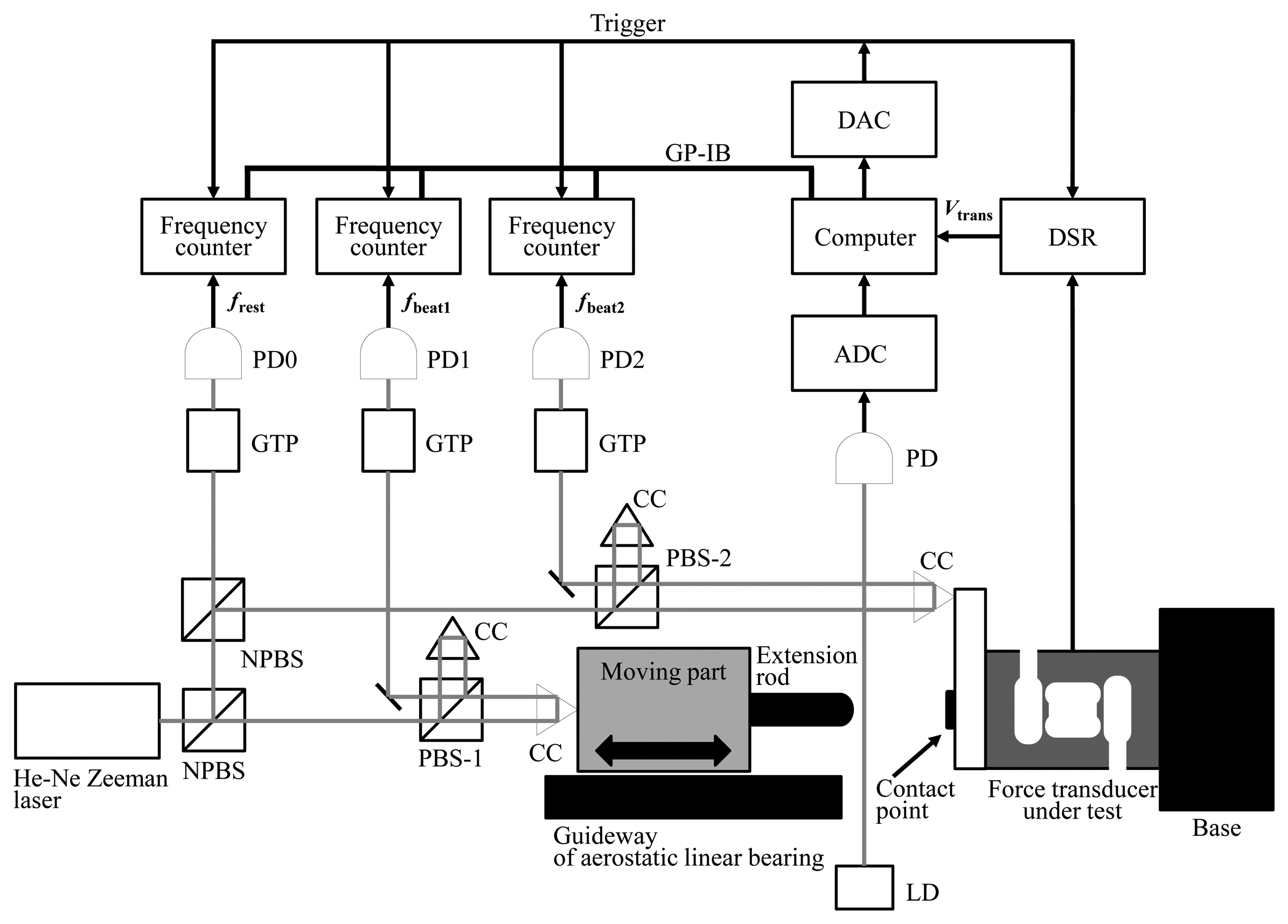
Figure 1 shows schematic diagram of the experimental setup for measuring the impact response of force transducers. The transducer under test is fixed on a large metal base of 10³ kg. An aerostatic linear bearing is used in order to obtain a linear motion with sufficiently small friction acting on the mass, i.e., the moving part of the bearing. The initial velocity is given to the moving part by hand.

A rubber block of sufficiently small mass is attached at the sensing point in order to adjust the steepness of the impact. The velocity of the mass v₁ and the velocity of the sensing point of the transducer v₂ are measured using two optical interferometers named Interferometer-1 and Interferometer-2, respectively. The force acting on the sensing point is obtained by the equation of motion, F = ma, where m is the mass and a is the acceleration.

The mass of the moving part including the cube corner prism (CC) and the extension rod, M₁, is approximately 2.653 kg. The mass of the contact point of the transducer, including the CC and their base plate, M₂, is approximately 0.082 kg.

Three conventional S-shaped strain-gage type transducers (model: DB-200N, capacity: 200N manufacturer: Showa Measuring Instruments Co. Ltd., Tokyo, Japan)—Transducer-1, Thransducer-2 and Transducer-3—are used in the experiment. The year of manufacture of Transducer-1 is 2000, and that of the other two transducers is 2008.

A Zeeman-type two-frequency He-Ne laser is used as the light source of the optical interferometers. The interferometers have three photo-detectors: PD0, PD1 and PD2. The frequency difference between the two orthogonal polarization states emitted from the laser, f_rest, is monitored using a Glan-Thompson prism (GTP) and the first photo-detector, PD0.

The total force acting on the moving part of the aerostatic linear bearing, F_mass, is calculated as the product of its mass, M₁, and its acceleration, a₁, as follows:

$$F_{\text{mass}}=M_1{a}_1$$

(1)

In the measurement, the total force acting on the mass, F_mass, is considered to be the same as the force acting on the mass from the force transducer being tested, since the frictional force acting on the mass is negligible [7]. The acceleration is calculated from the velocity of the levitated mass. The velocity of the mass, i.e., of the moving part of the aerostatic linear bearing, v₁, is measured as the Doppler shift frequency, f_Doppler1, which can be expressed as follows:

$$v_1={\mathrm{\lambda }}_{\text{air}}(f_{\text{Doppler}1})/2$$

(2)

$$f_{\text{Doppler}2}=-(f_{\text{beat}1}-f_{\text{rest}})$$

(3)

where λ_air is the wavelength of the signal beam under the experimental conditions, and f_beat1 is the beat frequency, which is the frequency difference between the signal beam and the reference beam and appears as the beat frequency at PD1. The position of the mass x₁, the acceleration of the mass a₁ and the force acting on the mass, F_mass, are numerically calculated from the velocity.

On the other hand, the velocity of the sensing point of the force transducer, v₂, is measured as the Doppler shift frequency, f_Doppler2, which can be expressed as follows:

$$v_2={\mathrm{\lambda }}_{\text{air}}(f_{\text{Doppler}2})/2$$

(4)

$$f_{\text{Doppler}2}=-(f_{\text{beat}2}-f_{\text{rest}})$$

(5)

The beat frequency f_beat2 is measured using PD2. The position x₂ and the acceleration a₂ of the actuator are numerically calculated from the velocity v₂.

For simultaneous measurement, three frequency counters and the dynamic strain recorder (DSR) are triggered by a single signal originated by a light switch composed of a laser diode (LD) and a PD.

The force measured by the transducer, F_trans, is calculated using the output signal of the transducer V_trans stored by a dynamic strain recorder (DSR; model: DC-204R, Tokyo Sokki Kenkyujo, Tokyo, Japan) and its static calibration result. The force calculated using the output signal of the transducer and its static calibration result, F_trans is compared with the force measured as the inertial force of the mass, F_mass.

In the experiments, one set of experiment consists of 20 impact measurements. The first set of the experiments using Transducer-1, Set_A1, is conducted for evaluating the parameters for dynamic error correction. Then, additional three sets of experiments using all the three transducers are conducted for evaluating the validity of the estimated parameters. These additional three sets of the experiments using Transducer-1, Transducer-2 and Transducer-3, are described as Set_B1, Set_B2 and Set_B3, respectively.

3. Estimation of the Parameters for Dynamic Error Correction

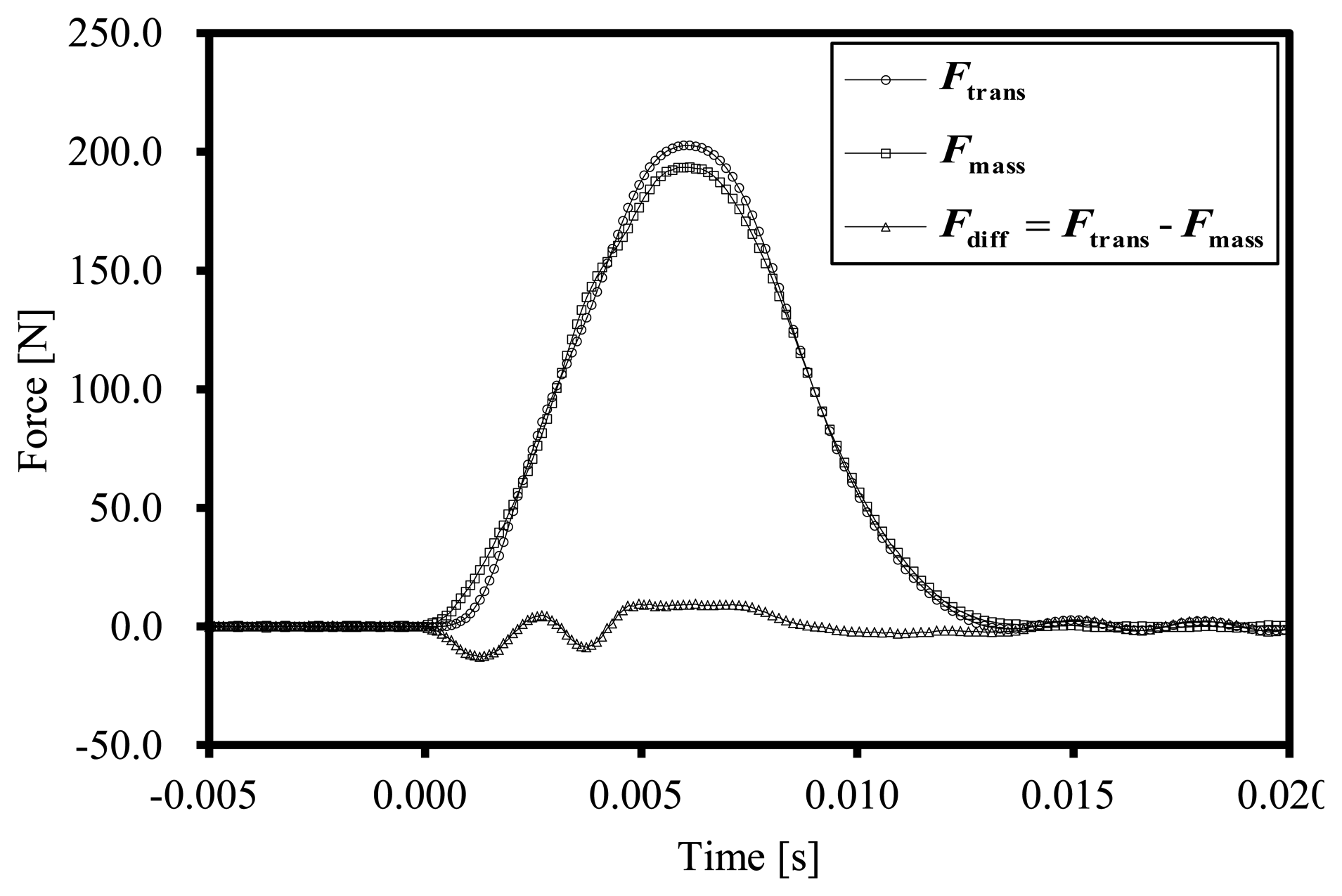
Figure 2 shows the result of a single set of the impact tests of Transducer-1. Figure 2 shows the force measured by the force transducer F_trans, and the force acting on the mass F_mass and their difference F_diff:

$$F_{\text{diff}}=F_{\text{trans}}-F_{\text{mass}}$$

(6)

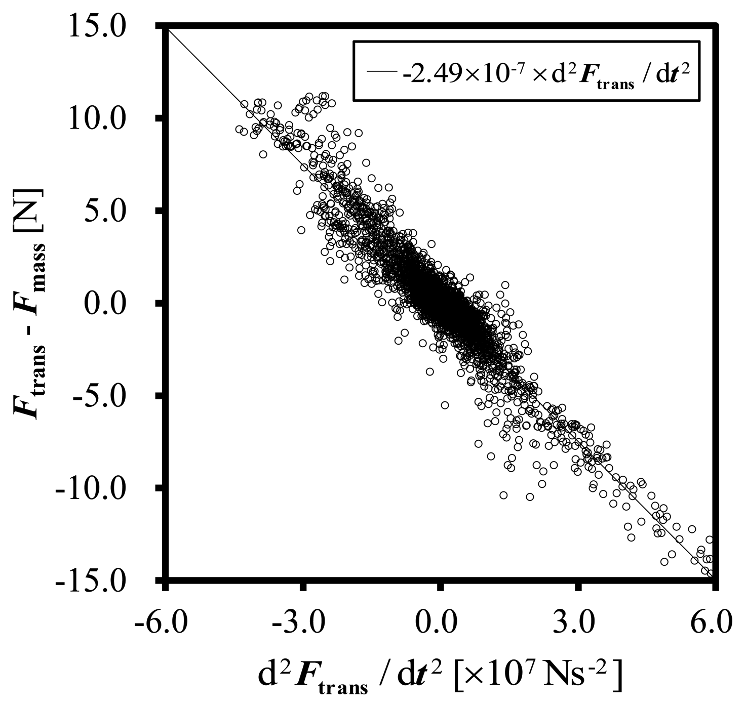
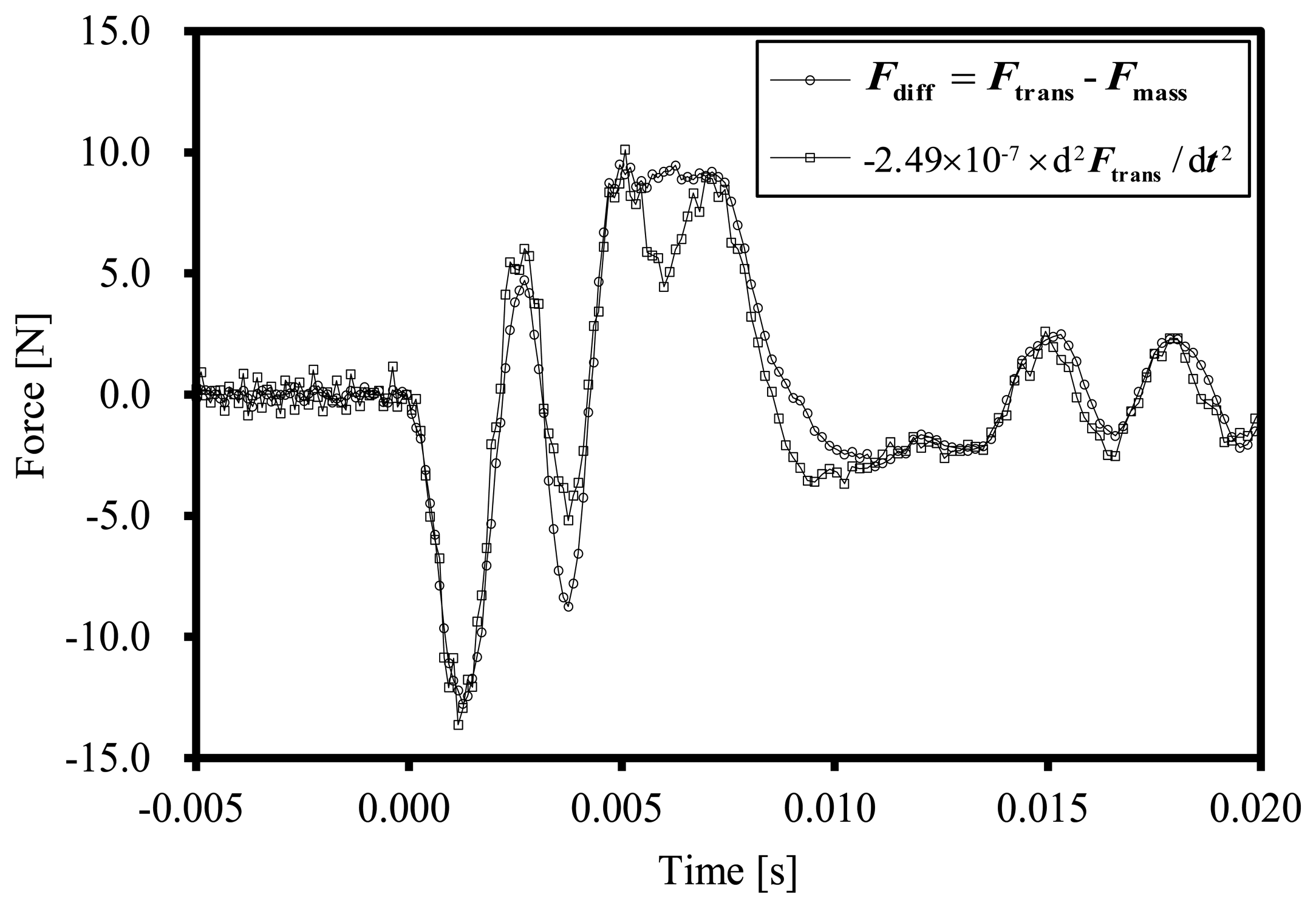
The figure shows the electric response of the force transducer under the impact load. The difference between F_trans and F_mass is derived mainly from the difference between the static and dynamic characteristics of the transducer. The root mean square (RMS) value of the difference between F_trans and F_mass during the collision period, 0 ms < t < 14 ms, was approximately 6.2 N. Figure 3 shows the relationship between the second time derivative of the force measured using the force transducer, d²F_trans/dt², and F_diff, for Set_A1.

The plots show a linear relationship between d²F_trans/dt² and F_diff. The solid line in Figure 3 shows a regression line of the following equation.

$$F_{\text{reg}}=C({\text{d}}^2{F}_{\text{trans}}/\text{d}{t}^2)$$

(7)

The parameter for dynamic error estimation C is obtained as the slope of the regression line. Here, the regression line is determined by a least-square method and resulted in C = −2.49 × 10⁻⁷ s². The measured plots coincide well with the regression line.

Figure 4 shows the difference between F_trans and F_mass and inertial forces of the transducer estimated with the parameter C, F_reg. The measurement error, F_diff, is almost the same as the result of the regression analysis, F_reg. From this result, the corrected force, F_corrected, can be calculated using following equation:

$$F_{\text{corrected}}=F_{\text{trans}}-F_{\text{reg}}=F_{\text{trans}}-C({\text{d}}^2{F}_{\text{trans}}/\text{d}{t}^2)=F_{\text{trans}}-(-2.49\times {10}^{-7})({\text{d}}^2{F}_{\text{trans}}/\text{d}{t}^2)$$

(8)

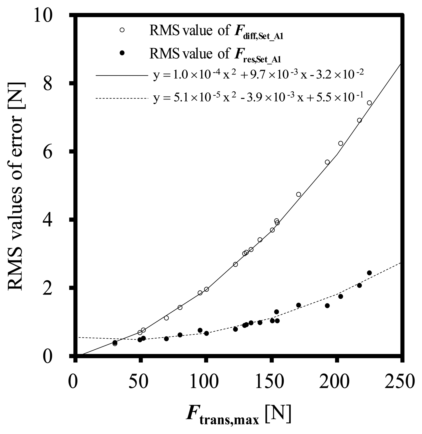
Figure 5 shows RMS values of the dynamic errors F_diff and that of residual errors after dynamic correction F_res:

$$F_{\text{res}}=F_{\text{corrected}}-F_{\text{mass}}$$

(9)

for Set_A1. The RMS values of F_diff and F_res seem to be almost square functions of the maximum force F_trans,max.

Solid and dashed curves in Figure 5 are regression curves of the RMS values of F_diff and F_res, respectively. The RMS value of the differences between F_diff and its regression line and that between F_res and its regression line are 1.34 × 10⁻¹ N and 3.58 × 10⁻¹ N, respectively. This results show that the RMS values of the F_diff and F_res can be estimated from the F_trans,max.

4. Evaluation of the Validity of the Estimated Parameters

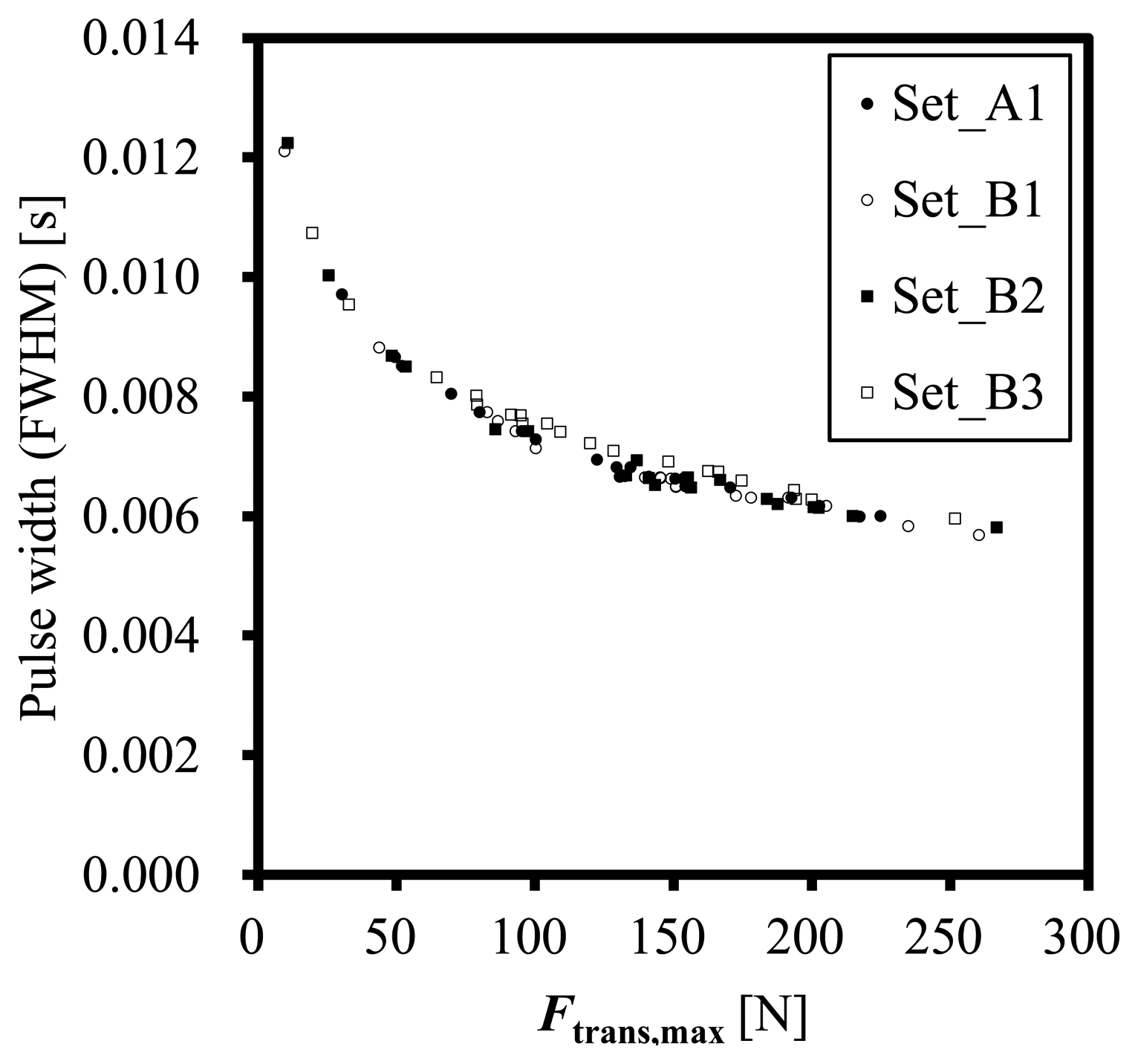
To evaluate the validity of the dynamic error correction using the parameter C estimated using Transducer-1, the dynamic error correction is applied to the other sets of experiments performed by the three transducers, i.e., Set_B1, Set_B2 and Set_B3. Figure 6 shows relations between the full width at half maximum (FWHM) of F_trans and the maximum force, F_trans,max for all the four sets of the experiments. All the sets show the similar relation.

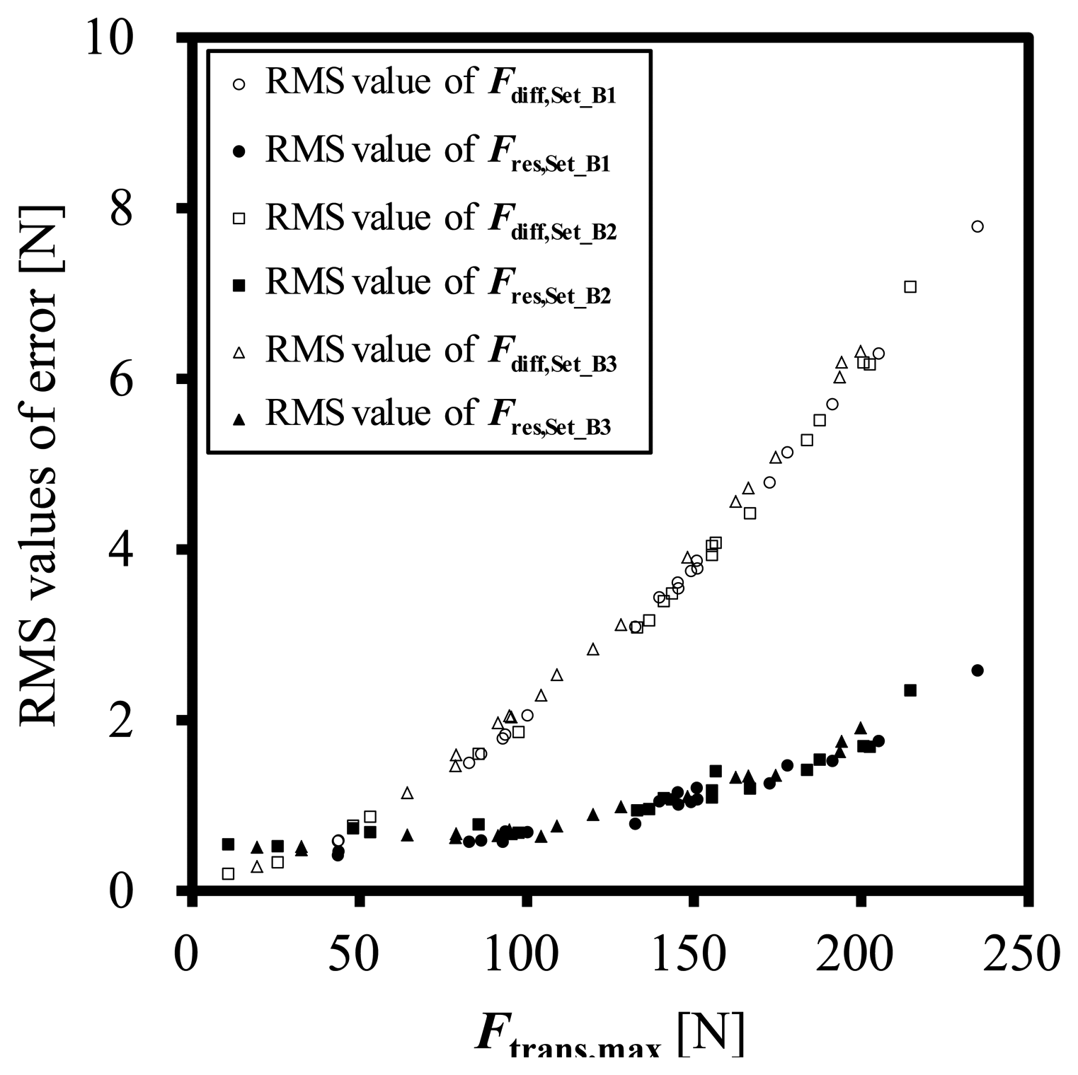
Figure 7 shows the RMS values of the dynamic error F_diff and that of residual error after dynamic correction F_res, about Set_B1, Set_B2 and Set_B3. The RMS values of F_res are effectively smaller than that of F_diff. The correction with the parameter C has enough of a result even though Transducer-1 is 8 years older than the other two transducers.

5. Estimation of Uncertainty

The standard uncertainty u_trans in the un-corrected force F_trans is estimated as follows:

$${\mathit{\text{u}}}_{\mathbf{\text{trans}}}=\sqrt{{{\mathit{\text{u}}}_{\mathbf{\text{diff}}}}^2+{{\mathit{\text{u}}}_{\mathbf{\text{LMM}}}}^2}$$

(10)

where u_diff is the RMS value of F_diff during the impact shown in Figure 5. In the experiments, u_LMM is estimated to be 1.2 × 10⁻⁴ N[7] and is negligible. As shown in Figure 5, the u_diff can be assumed as a square function of the peak value of the force F_trans,max as follows:

$${\mathit{\text{u}}}_{\mathbf{\text{trans}}}={\mathit{\text{E}}}_{\mathbf{\text{S}}\mathbf{,}\mathbf{1}}·{\mathit{\text{F}}}_{\mathbf{\text{trans}}\mathbf{,}\mathbf{\text{max}}}^2+{\mathit{\text{E}}}_{\mathbf{\text{S}}\mathbf{,}\mathbf{2}}·{\mathit{\text{F}}}_{\mathbf{\text{trans}}\mathbf{,}\mathbf{\text{max}}}+{\mathit{\text{E}}}_{\mathbf{\text{S}}\mathbf{,}\mathbf{3}}$$

(11)

where the constants E_S,1, E_S,2 and E_S,3 are parameters for estimating the dynamic error in the un-corrected force F_trans calculated based on the conventional static calibration.

As same as the u_trans, the standard uncertainty u_corrected in the corrected force F_corrected is estimated as follows:

$${\mathit{\text{u}}}_{\mathbf{\text{corrected}}}=\sqrt{{{\mathit{\text{u}}}_{\mathbf{\text{res}}}}^2+{{\mathit{\text{u}}}_{\mathbf{\text{LMM}}}}^2}$$

(12)

where u_res is the RMS value of the residual error F_res during the impact shown in Figure 5. The u_res can be assumed as a square function of the peak value of the force F_trans,max as follows:

$${\mathit{\text{u}}}_{\mathbf{\text{corrected}}}={\mathit{\text{E}}}_{\mathbf{\text{D}}\mathbf{,}\mathbf{1}}·{\mathit{\text{F}}}_{\mathbf{\text{trans}}\mathbf{,}\mathbf{\text{max}}}^2+{\mathit{\text{E}}}_{\mathbf{\text{D}}\mathbf{,}\mathbf{2}}·{\mathit{\text{F}}}_{\mathbf{\text{trans}}\mathbf{,}\mathbf{\text{max}}}+{\mathit{\text{E}}}_{\mathbf{\text{D}}\mathbf{,}\mathbf{3}}$$

(13)

where the constants E_D,1, E_D,2 and E_D,3 are parameters for estimating the residual error in the corrected force F_corrected estimated by means of the proposed dynamic correction method.

6. Correction Software

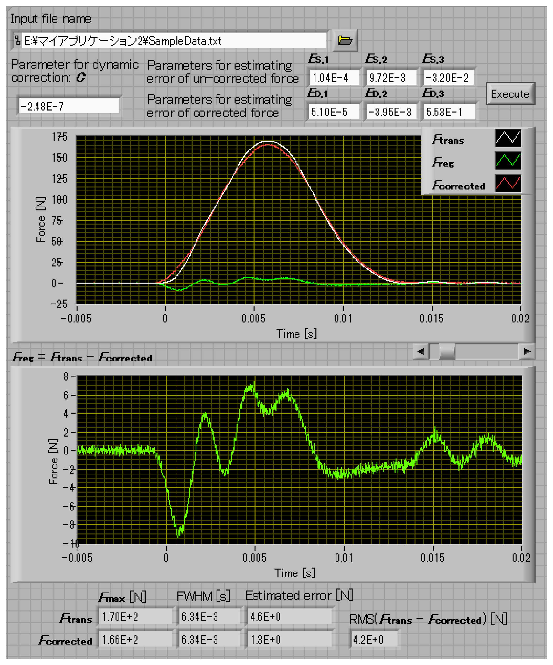
From the knowledge obtained from the above experiments, software that corrects the dynamic error in the impact force measurement is developed [8]. It works in the Microsoft Windows environment. Figure 8 shows a screenshot of the software.

This software processes the input waveform measured by the transducer based on the static calibration result, F_trans, into (a) waveform of dynamic error F_reg [= C(d²F_trans/dt²)]; (b) waveform of corrected force F_corrected (= F_trans − F_reg); In addition, this software calculates: (c) the standard uncertainty u_trans in the un-corrected force F_trans; and (d) the standard uncertainty u_corrected in the corrected force F_corrected.

The software outputs them to a output file and shows them to the monitor window. The format of the input waveform file is a text format described the sampling interval in time and the sequence of force in newton calculated based on the static calibration result. The format of the output data file is a CSV format. The input data and the output data of the developed software are as follows,

(A)

Input data, which should be manually input from the operational window.

(1)

Name of input text-file, in which the data set of the force calculated based on the static calibration results F_trans(i) with the measurement time t(i) contains: [t(i), F_trans(i)] (0 ≤ i < N − 1).

(2)

Parameter for dynamic error correction: C.

(3)

Parameters for estimating the dynamic error in the un-corrected force F_trans calculated based on the conventional static calibration: E_S,1, E_S,2 and E_S,3.

(4)

Parameters for estimating the residual error in the corrected force F_corrected estimated by means of the proposed dynamic correction method: E_D,1, E_D,2 and E_D,3.

(B)

Output data, which is written in a CSV-file and shown on the display:

(1)

Waveform of F_trans, F_reg [= C(d²F_trans/dt²)] and F_corrected (= F_trans − F_reg).

(2)

Parameters for F_trans: the maximum value F_trans,max, the pulse width FWHM_trans and estimated error u_trans.

(3)

Parameters for F_corrected: the maximum value F_{corrected,max}, the pulse width FWHM_corrected and estimated error u_corrected.

(4)

RMS value of the difference between F_trans and F_corrected.

7. Conclusion

The validity of the proposed method for correcting the dynamic error in the impact force measurement is experimentally evaluated using three force transducers of the same model. Based on the experimental results, software, which corrects the dynamic error of force transducers using their own output signal, has been developed. Because there are no dynamic calibration methods for force transducers available at this moment, we believe that the work described in this paper is very valuable.

There are, however, still residual errors in the corrected force. For example, there is a small error factor which is assumed to result from the viscosity of the internal structure of the transducer. For more accurate correction and more accurate estimation of the uncertainty of measurement, our group is working on more accurate measurement of the force with the LMM and investigating the causes of the residual errors. Additionally, we will apply this correction method to transducers of other types and other models with wider ranges of forces in the future.

In this paper, the dynamic error correction is performed considering only with the inertial force of a part of the transducer itself. If a certain part is attached to the sensing point of the transducer and the force acting to the opposite side of the attached part should be measured, then the correction parameter should be modified for the mass of the attached part.

If the sensor manufacturers were to determine the correction parameters for each model using the proposed method; and provide the software with the parameters corresponding to each model; then the users could obtain waveforms corrected against dynamic errors and their uncertainty. We believe that in the near future; all the manufacturers of force transducers will provide similar software and the parameters corresponding to their products, so that transducer users will be able to perform dynamic error corrections and remove their uncertainty easily.

References

- Fujii, Y. Toward establishing dynamic calibration method for force transducers. IEEE Trans. Instrum. Meas. 2009, 58, 2358–2364. [Google Scholar]
- Djamal, M.; Watanabe, K.; Irisa, K.; Prayogi, I.; Takita, A.; Yamaguchi, T.; Fujii, Y. Dynamic characteristics measurements of a force transducer against small and short-duration impact forces. Metrol. Meas. Syst. 2014, 21, 59–66. [Google Scholar]
- Xu, K.-J.; Jia, L. One-stage identification algorithm and two-step compensation method of Hammerstein model with application to wrist force sensor. Rev. Sci. Instrum. 2002, 73, 1949–1955. [Google Scholar]
- Fujii, Y. Measurement of the electrical and mechanical responses of a force transducer against impact forces. Rev. Sci. Instrum. 2006, 77, 085108. [Google Scholar]
- Fujii, Y. Method for correcting the effect of the inertial mass on dynamic force measurements. Meas. Sci. Technol. 2007, 18, N13–N20. [Google Scholar]
- Fujii, Y.; Maru, K. Self-correction method for dynamic measurement error of force sensors. Exp. Tech. 2011, 35, 15–20. [Google Scholar]
- Fujii, Y. Frictional characteristics of an aerostatic linear bearing. Tribol. Int. 2006, 39, 888–896. [Google Scholar]
- Fujii Lab Homepage. Available online: http://www.el.gunma-u.ac.jp/∼fujii/main_e.htm (accessed on 4 July 2014).
© 2014 by the authors; licensee MDPI, Basel, Switzerland. This article is an open access article distributed under the terms and conditions of the Creative Commons Attribution license ( http://creativecommons.org/licenses/by/3.0/).
Share and Cite
Miyashita, N.; Watanabe, K.; Irisa, K.; Iwashita, H.; Araki, R.; Takita, A.; Yamaguchi, T.; Fujii, Y. Software for Correcting the Dynamic Error of Force Transducers. Sensors 2014, 14, 12093-12103. https://doi.org/10.3390/s140712093
Miyashita N, Watanabe K, Irisa K, Iwashita H, Araki R, Takita A, Yamaguchi T, Fujii Y. Software for Correcting the Dynamic Error of Force Transducers. Sensors. 2014; 14(7):12093-12103. https://doi.org/10.3390/s140712093
Chicago/Turabian StyleMiyashita, Naoki, Kazuhide Watanabe, Kyouhei Irisa, Hiroshi Iwashita, Ryosuke Araki, Akihiro Takita, Takao Yamaguchi, and Yusaku Fujii. 2014. "Software for Correcting the Dynamic Error of Force Transducers" Sensors 14, no. 7: 12093-12103. https://doi.org/10.3390/s140712093
APA StyleMiyashita, N., Watanabe, K., Irisa, K., Iwashita, H., Araki, R., Takita, A., Yamaguchi, T., & Fujii, Y. (2014). Software for Correcting the Dynamic Error of Force Transducers. Sensors, 14(7), 12093-12103. https://doi.org/10.3390/s140712093