Cooperative MIMO Communication at Wireless Sensor Network: An Error Correcting Code Approach

Abstract
: Cooperative communication in wireless sensor network (WSN) explores the energy efficient wireless communication schemes between multiple sensors and data gathering node (DGN) by exploiting multiple input multiple output (MIMO) and multiple input single output (MISO) configurations. In this paper, an energy efficient cooperative MIMO (C-MIMO) technique is proposed where low density parity check (LDPC) code is used as an error correcting code. The rate of LDPC code is varied by varying the length of message and parity bits. Simulation results show that the cooperative communication scheme outperforms SISO scheme in the presence of LDPC code. LDPC codes with different code rates are compared using bit error rate (BER) analysis. BER is also analyzed under different Nakagami fading scenario. Energy efficiencies are compared for different targeted probability of bit error pb. It is observed that C-MIMO performs more efficiently when the targeted pb is smaller. Also the lower encoding rate for LDPC code offers better error characteristics.1. Introduction
Recent advances in micro-electro-mechanical systems technology have enabled the development of wireless sensor nodes in a wireless sensor network (WSN). These tiny sensor nodes are able to sense, process and communicate with each other [1,2]. Since the battery capacity in each node is limited and the goal is to maximize the lifetime of the network, there are strict energy consumption constraints in WSNs [3]. The size of sensors is typically small but the functions inside the sensor are complex. Recent hardware advancements allow more signal processing functionality to be integrated into a single sensor chip. RF transceiver, A/D and D/A converters, base band processors, and other application interfaces are integrated into a single device to be used as a smart wireless node. A wireless sensor network typically consists of a large number of sensor nodes distributed over a certain region. Monitoring node (MN) monitors its surrounding area, gathers application-specific information, and transmits the collected data to a data gathering node (DGN) or a gateway. Energy issues are more critical in the case of MNs rather than in the case of DGNs since MNs are remotely deployed and it is not easy to frequently change the energy sources. Therefore, the MNs have been the principal design issue for energy limited wireless sensor network design. One prospective solution is the use of MIMO [4,5] for energy efficient design with a targeted probability of bit error at the receiver. Also LDPC-coded MIMO optical communication is mentioned in [6]. But the MIMO techniques require complex transceiver circuitry and signal processing leading to large power consumptions at the circuit level. Moreover, physical implementation of multiple antennas at a small-size sensor node may not be feasible. The solution came in the form of cooperative MIMO (C-MIMO) [4–8]. C-MIMO is a kind of MIMO technique where the multiple inputs and outputs are formed via cooperation in a network of single antenna nodes. The sensors cooperate with each other to form a MIMO structure and in fact lead to better energy efficiency and smaller end-to-end delay. The basic idea of C-MIMO was first proposed by S. Cui in [4]. Later this idea has been improved in [5] by Jayaweera considering channel estimation (training overhead) in the DGN side and is further modified in [9] by Y. Gai and in [8] by M. Rakibul.
The issue of applying error control codes in WSNs is the topic of recent interest. The performance of block codes and Viterbi decoded convolutional codes is investigated in [10,11]. The iterative decoding algorithm using turbo code is used to prolong the network lifetime [12]. Low-density parity-check (LDPC) codes are more reliable than the block and convolutional codes and are serious competitors of turbo codes. In particular, LDPC codes exhibit an asymptotically better performance than turbo codes and admit a wide range of trade-offs between performance and decoding complexity [13]. Sartipi and Fekri [14] compare the performance of the LDPC codes and the Reed Solomon (RS) codes [15]. From the recent works, it is known that LDPC codes are attractive in WSNs because of their applications in compression, joint sourcechannel coding and distributed source coding [14,16]. However, to the best knowledge of the authors, there has been no document on the implementation of LDPC encoder/decoder in a wireless sensor node using cooperative communication. More precisely, none of the recent works have addressed the problem of reducing the energy consumption using error control coding. In this paper, LDPC code is incorporated in cooperative communication as an error control code. Later the idea is compared with SISO communication. In Section 2, the system model is shown and the error correction using LDPC code is analyzed in Section 3. Section 4 shows the energy model for both cooperative MIMO and SISO considering error correction codes. In Section 5, simulation results are shown and discussed. Finally, Section 6 concludes the paper.
2. Cooperative MIMO Communication
2.1. System Model
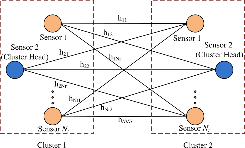
The system model for C-MIMO communication is a centralized wireless sensor network where there is a data gathering node (DGN) and several clusters with several sensors in each cluster. Sensors in one cluster transmit the data to the sensors in adjacent cluster and step by step the data reach the DGN. Figure 1 shows the cluster to cluster communication where two clusters are shown. The system considers Nt number of sensors in the transmitting cluster, Nr number of sensors in the receiving cluster and one antenna is placed at one sensor. Also, each element in the channel matrix H is assumed to be a zero-mean circularly symmetric complex Gaussian random variable with unit variance and can be considered as follows.
The problem here is stated from the receiver point of view, so a loss model is used to estimate the received energy. To calculate the total energy consumption, both the circuit and transmitter power are taken into count. The same transmitter and receiver blocks shown in [4] are used in this paper. Source coding, pulse shaping, and modulation block are as well omitted from the design. Throughout the paper, a system with narrowband, frequency-flat Rayleigh fading channels and perfectly synchronized transmission/reception between wireless sensor nodes is assumed. The fading is assumed constant during the transmission of each frame. In our model, a sensor with high residual energy is deployed as a cluster head and it remains the cluster head until the network dies. The cluster head broadcasts its status to the other sensors in the network. Each sensor node determines to which cluster it wants to belong by choosing the cluster head that requires the minimum communication energy. Once all the nodes are organized into clusters, each cluster head creates a schedule for the nodes in its cluster. This allows the radio components of each non-cluster-head node to be turned off at all times except during its transmit time, thus minimizing the energy dissipated in the individual sensors.
2.2. Cooperative Communication
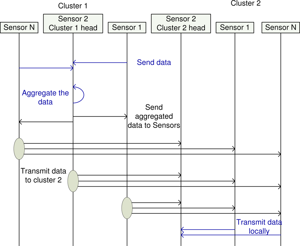
The physical phenomena monitored by sensor networks, e.g., forest temperature, water contamination, usually yield sensed data that are strongly correlated. Data aggregation is the tool by which the correlated data size can be significantly reduced depending on the correlation factor. Figure 2 explains the cooperative communication where the sensors at cluster 1 send the information data to the cluster head os cluster 2. At the first step, the sensors at cluster 1 send the data to their cluster head. The cluster head then aggregates the data in the second step. After the aggregation, the cluster head send the aggregated data back to all the sensors in that cluster. This is the step three in cooperative communication. At this stage, all the sensors at cluster 1 have the same information data. At the fourth step, the sensors transmit the aggregated data to the cluster 2. After receiving the data at the receiving cluster, sensors at cluster 2 transmit the received data to their cluster head locally and complete the cooperative communication.
3. Error Correction Codes in Wireless Sensor Network
Error control coding (ECC) introduces redundancy into an information sequence u of length k by the addition of extra parity bits. Several different types of ECC exist, but we may loosely categorize them into two divisions: (1) block codes, which are of a fixed length nC, with nC − k parity bits, and are decoded into one block or codeword at a time; (2) convolutional codes, which, for a rate k/nC code, input k bits and output nC bits at each time interval, but are decoded in a continuous stream of length L >> nC. Block codes include repetition codes, Hamming codes [17], Reed Solomon codes, and BCH codes [18]. Short block codes like Hamming codes can be decoded by syndrome decoding or maximum likelihood (ML) decoding by either decoding to the nearest codeword or decoding on a trellis with the Viterbi algorithm or maximum a posteriori (MAP) decoding with the BCJR algorithm. Algebraic codes such as Reed Solomon and BCH codes are decoded with a complex polynomial solver to determine the error locations. Convolutional codes are decoded on a trellis using either Viterbi decoding, MAP decoding, or sequential decoding.
Another categorization is based on the decoding algorithms: (1) non-iterative decoding algorithms, such as syndrome decoding for block codes or maximum likelihood (ML) nearest codeword decoding for short block codes, algebraic decoding for Reed Solomon and BCH codes, and Viterbi decoding or sequential decoding for convolutional codes; (2) iterative decoding algorithms, such as turbo decoding with component MAP decoders for each component code, and the sum product algorithm (SPA) [19] or its lower complexity approximation, min-sum decoding [20], for low density parity check codes (LDPCs). The non-iterative decoding category may be further divided into hard and soft decision decoders; hard decision decoders output a final decision on the most likely codeword, while soft decision decoders provide soft information in the form of probabilities or log-likelihood ratios (LLRs) on the individual codeword bits. Viterbi decoding can be either hard decision or soft decision, with a 2dB gain in performance for soft decision decoding. Category (2) are all soft decision algorithms by nature, as iterative decoding requires soft information as a priori input for each iteration. Iterative decoding algorithms provide significant coding gain, at the cost of greater decoding complexity and power consumption. With the recent technological advancements, all these ECC techniques can be used in WSN. However, LDPC code is considered in this paper as an ECC tool at WSN for its superior error correcting capabilities.
3.1. Low Density Parity Check Codes
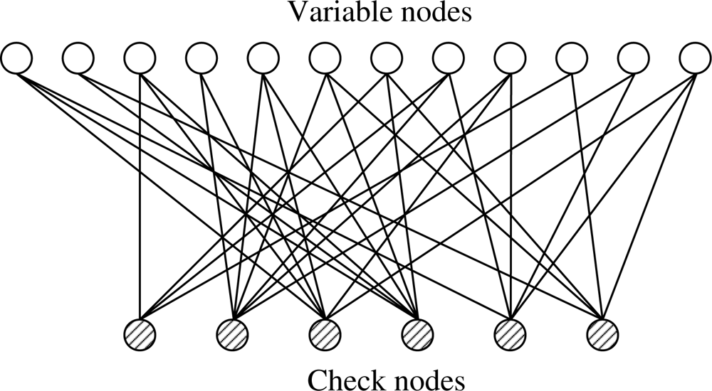
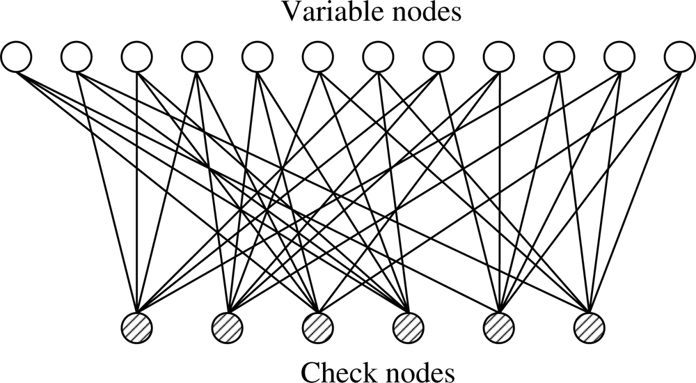
Low density parity check codes are codes specified by a matrix containing mostly 0’s and relatively few 1’s. A standard bipartite graph based ensemble which is shown in [21,22] is used in this paper. The code length is designated by n and number of constraints by m. Therefore, there are n variable nodes and m check nodes. Each variable node corresponds to one bit of the codeword and each check node corresponds to one parity check equation. Edges in the graph connect variable nodes to check nodes and represents the nonzero entries in H matrix. The term “low density” conveys the fact that the fraction of nonzero entries in H is small, in particular it is linear in the block length n, as compared to “random” linear codes for which the expected fraction of ones grows like n2 [23].
For regular codes, the corresponding H matrix has δr ones in each row and δc ones in each column. It means that every codeword bit participates in exactly δc parity-check equations and that every such check equation involves exactly δr codeword bits. Low density parity check codes have been constructed mostly using regular random bipartite graphs.
Example 1. Here is an example of a regular parity check matrix with δr = 6 and δc = 3.
The bipartite graph corresponding to this parity check matrix is shown in Figure 3.
For irregular codes, δr and δc are not fixed for every row and column of the parity check matrix. We consider that the irregular bipartite graph has a maximum variable side degree δr and a maximum check side degree δc.
Example 2. The following H matrix is an example of an irregular parity check matrix with a maximum δr = 6 and a maximum δc = 3.
The bipartite graph corresponding to this parity check matrix is shown in Figure 4.
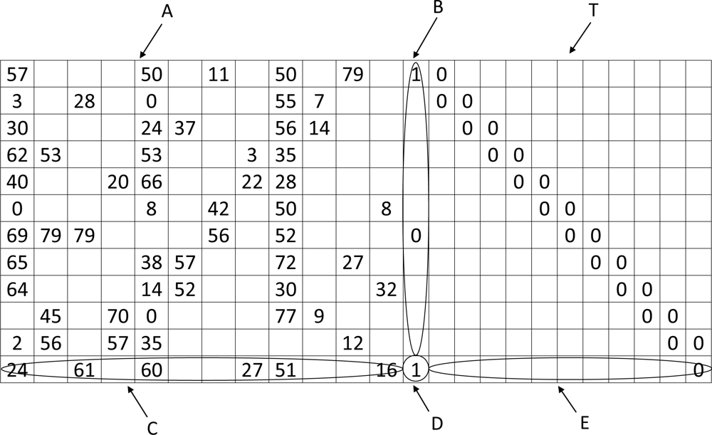
For this paper, H matrix shown in Figure 5 is used for simulation. This H matrix is a special matrix used in 802.11n standard. WSN is energy constraint in nature and the sensors work as intermediate devices when the data are transferred from a designated area to the data gathering node (DGN). Since decoding can be performed in the DGN, energy efficient decoding technique is not a concern for this paper. Encoding is one critical issue considered in the wireless sensor network. In this paper, Richardson encoding scheme is used as a tool for using LDPC code in WSN and is explained in the next subsection.
3.2. Richardson Scheme as the Encoding Technique
The encoding method proposed by Richardson et al. [13] assumes that H can be converted to an approximate lower triangular matrix. The authors worked on an m × n parity check matrix H over F where n is the number of variable nodes and m is the number of check nodes. The parity check matrix H is transformed in the form of
And the H matrix is found as
They then break the codeword as x = (s, p1, p2) where s denotes the systematic part, p1 and p2 denote the parity part, p1 has length g, and p2 has length (m − g). After that, the equation HxT = 0T is used to state the following two equations
Taking (−ET−1B + D) as nonsingular, it is concluded that
By using the step by step procedure, it is shown that the complexity of calculating p1 and p2 are O(n + g2) and O(n) respectively. The matrix used in our simulation can also be written in ALT form and is shown in Figure 5.
4. Energy Model for Cooperative Communication Using LDPC Code
The total power consumption PT for a single node consists of two main parts, namely, the power consumption of all the power amplifiers PPA which is a function of transmission power Pout, and the power consumption of all other circuit blocks PC. Thus one can write
The power consumption in the circuit block includes transmitter and receiver power consumption Pct and Pcr, respectively. This power consumption is due to several power blocks such as Pmix, Psyn, Pfilt, Pfilr, PLNA, PIFA, PDAC, and PADC which are the power consumption values of the mixer, the frequency synthesizer, the active filters at the transmitter and at the receiver side, the low noise amplifier, the intermediate frequency amplifier, the D/A and A/D converter, respectively. The power consumption block for error correction is not considered as it is same for cooperative case and SISO case. The total energy consumption per bit can be written as
The total energy consumption in cooperative case is modeled as
The energy per bit is needed to transmit the data from sensors to the cluster head. Eda is the energy dissipation per bit required in the cluster head for data aggregation. It depends on the algorithm complexity and can be expressed as
For the SISO approach, sensors transmit their data to the cluster head and as there is no burden for channel estimation, the cluster head will transmit all the aggregated data directly to the destination node without any cooperation. So the total energy consumption becomes
5. Simulation Results and Discussion
In order to get the total communication energy consumption, the average energy per bit required for a given BER Pb, Ēb needs to be determined. In this approach, the value of Ēb is found by using a numerical search. Ten thousand randomly generated channel samples are taken and averaged to find the desired bit error rate at each transmission distance. The value of the constellation size is kept fixed. For the long haul communication, SISO is taken as a special case of MIMO structure. A list of system parameters used in our simulation is shown in Table 1 where the power consumption values of various circuit blocks are quoted from [4].
5.1. Energy Issue
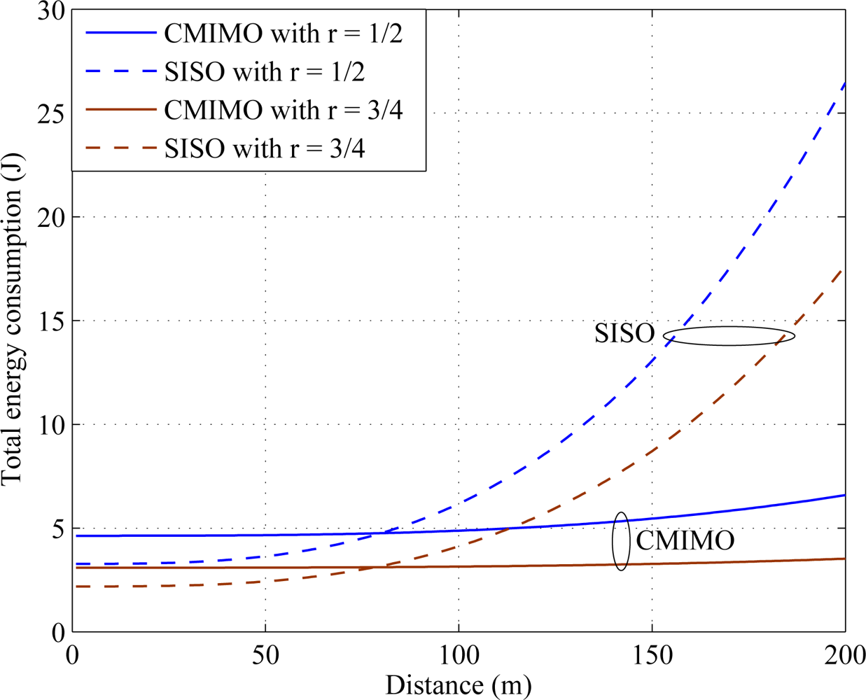
Total energy consumption and energy efficiency are the key terms to evaluate the energy efficient performance. For simulation, it is considered that all the sensors in a cluster are transmitting the same data size of Li = 10 kb. The simulation is performed based on the cluster size of Nt = 4. In Figure 6, the total energy consumption over distance is shown for cluster to cluster data transmission. From Figure 6 it is clear that the cooperative MIMO is more energy efficient than SISO transmission. The simulation is taken for two different code rates r = 1/2 and r = 3/4. When the code rate increases, parity bits compared to message bits are reduced. Therefore, total energy consumption reduces. This is verified in Figure 6.
5.2. Delay Issue
The total delay required is defined as the total transmission delay. For a fixed transmission bandwidth B, we assume that the symbol period is approximately TS ≈ 1/B. The total delays in the case of SISO communication is defined as
Where blt is the transmission bit size at the transmitter side local communication and bSISO is the transmission bit size for long haul SISO transmission. tda is the time taken for data aggregation.
The total delays in the case of cooperative MIMO communication is defined as
Where tch and tda are the channel estimation and data aggregation delays respectively. The term is for the delay due to the local transmission from sensors to the cluster head. The next term is due to the local transmission from cluster head to the sensors. term is caused by the long haul MIMO transmission. The next term is due to the local transmission at the receiver side. The assisting nodes first quantize each symbol they receive into nr bits, then transform all the bits into symbols using blr and transmit to the cluster head to do the joint detection.
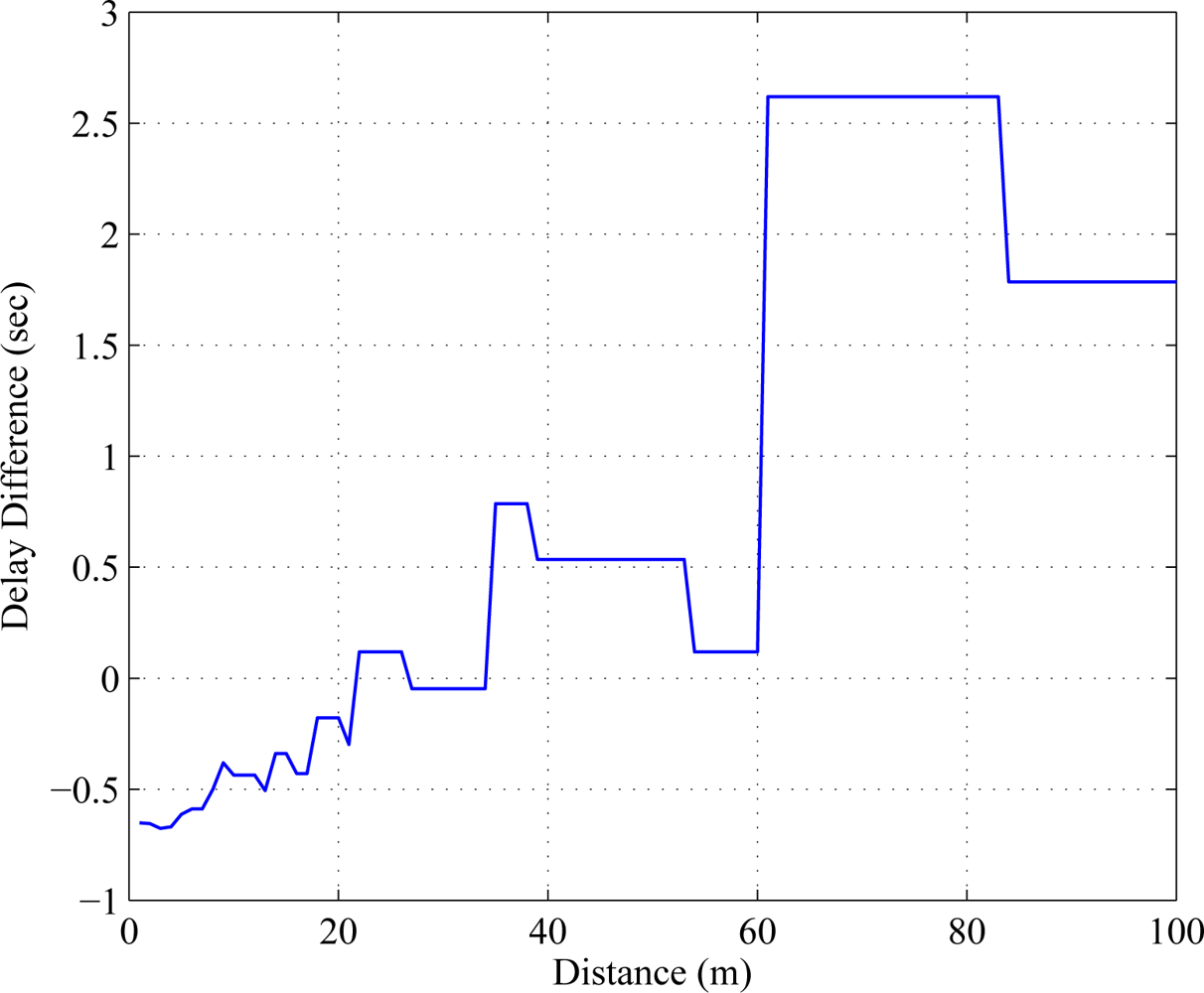
The delay difference is calculated using the following equation. We assume the value of tch ≈ 0.
The value of nr is chosen at the receiver based on the optimized transmitted constellation size. The delay difference is a measure of delay performance by which the cooperative MIMO can be compared with SISO. Positive delay difference indicates the SISO is facing larger delay compared to C-MIMO. In Figure 7, delay difference is compared where proposed C-MIMO outperforms SISO after 60 meters.
5.3. Constellation Size Issue
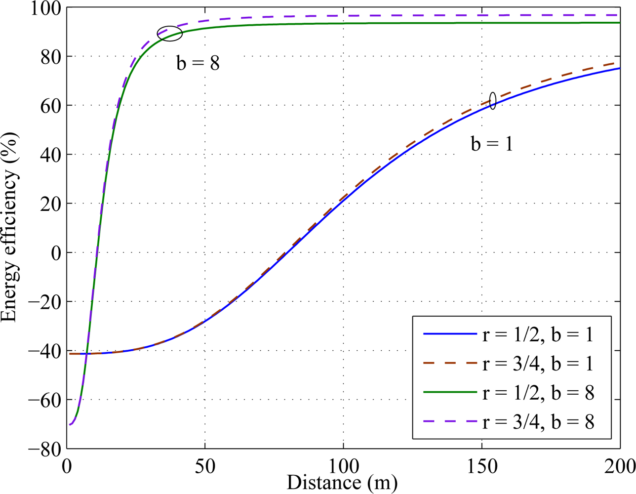
Since Energy efficiency = {ESISO − EC−MIMO}/ESISO, positive energy efficiency indicates {ESISO > EC−MIMO}. In Figure 8, energy efficiency is simulated over distance for different constellation sizes. The simulation results show that for rate r = 1/2, cooperative MIMO outperforms SISO after 80 meters for constellation size b = 1 whereas it takes 10 meters for constellation size b = 8.
5.4. Bit Error Rate Issue
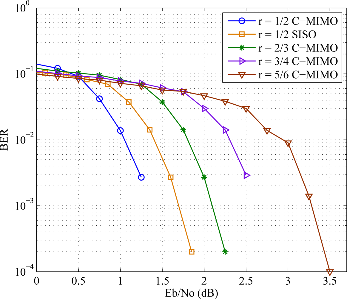
Using the parity check matrix provided in IEEE 802.11n standard shown in Figure 5, comparative error performance studies have been taken for different encoding rates and are shown in Figure 9. Also the C-MIMO is compared with SISO in the rate case. The codeword length is kept fixed and the number of decoder iteration is taken as 100. Bit error rate (BER) is taken as performance parameter in this paper. BPSK modulation and AWGN channel are used for the simulation. Like the other wireless channels, simulation using cooperative MIMO shows similar outcomes.
The same BER analysis is taken in Figure 10 in a Nakagami fading channel scenario. The result shows that the decrease in Nakagami coefficient m degrades the error performance.
5.5. Reception Quality Issue
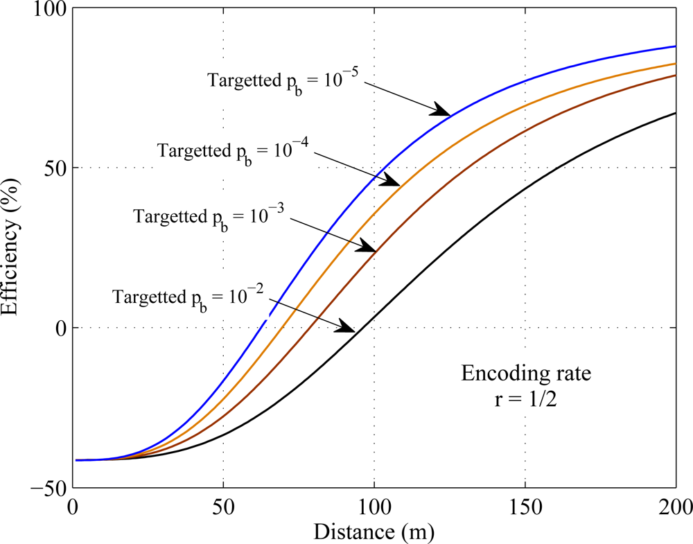
Targeted BER is the parameter that indicates the reception quality of the signal. The cooperative MIMO communication used in this paper is simulated with a fixed value of targeted BER. Figure 11 shows that the change in targeted BER changes the efficiency of cooperative communication over SISO transmission. Result shows that the cooperative communication is more energy efficient than SISO transmission in smaller targeted BER.
6. Conclusions
Energy efficient data transmission is one of the key factors for energy constraint wireless sensor network. An energy efficient cooperative technique considering low density parity check codes is modeled and simulated using Matlab. The results show that the cooperative communication outperforms SISO transmission at the presence of error correction code. The energy efficiency remains almost unchanged in different encoding rates but it largely varies with the change in constellation size. BER analysis is also taken to show the similar error characteristics in the cooperative MIMO environment. Data with smaller encoding rate shows better BER results than larger encoding rate for a fixed SNR. Simulation is also performed in the situation of a fading environment. It is also found that cooperative communication is more energy efficient than SISO transmission in smaller targeted BER. Therefore it can be concluded that cooperative MIMO with LDPC can be a good choice for high reception quality signals.
Acknowledgments
This work was supported by the Basic Research Program through the National Research Foundation of Korea (NRF) funded by The Ministry of Education, Science and Technology (2011-0379000).
References
- Anna, H. Wireless Sensor Network Design; John Wiley & Sons Ltd: Chichester, West Sussex, UK, 2003; p. 410. [Google Scholar]
- Akyildiz, I; Su, W; Sankarasubramaniam, Y; Cayirci, E. Wireless sensor networks: A survey. Comput. Netw. J 2002, 38, 393–422. [Google Scholar]
- Karvonen, H; Pomalaza-Raez, C. Coding for energy efficient multihop wireless sensor networks. Proceedings of Nordic Radio Symposium 2004/Finnish Wireless Communications Workshop 2004, (NRS/FWCW 2004), Oulu, Finland, 16–18 August 2004; pp. 1–5.
- Cui, S; Goldsmith, AJ; Bahai, A. Energy-efficiency of MIMO and cooperative MIMO techniques in sensor networks. IEEE J. Select. Areas. Commun 2003, 22, 1089–1098. [Google Scholar]
- Jayaweera, SK. Virtual MIMO-based cooperative communication for energy-constrained wireless sensor networks. IEEE Trans. Wirel. Commun 2006, 5, 984–989. [Google Scholar]
- Djordjevic, IB. LDPC-coded MIMO optical communication over the atmospheric turbulence channel using Q-ary pulse-position modulation. Opt. Express 2007, 15, 10026–10032. [Google Scholar]
- Li, X. Energy efficient wireless sensor networks with transmission diversity. IEEE Electron. Lett 2003, 39, 1753–1755. [Google Scholar]
- Islam, MR; Anh, HT; Kim, J. Energy efficient cooperative technique for IEEE 1451 based Wireless Sensor Network. Proceedings of IEEE Wireless Communications and Networking Conference (WCNC), Las Vegas, NV, USA, 31 March 2008.
- Gai, Y; Zhang, L; Shan, X. Energy Efficiency of cooperative MIMO with data aggregation in wireless sensor networks. Proceedigns of IEEE Wireless Communications & Networking Conference (WCNC), Hong Kong, China, 14 March 2007.
- Kashani, ZH; Shiva, M. BCH coding and multi-hop communication in wireless sensor networks. Proceedigns of Wireless and Optical Networks Conference (WOCN), Bangalore, India, 11–13 April 2006; pp. 1–5.
- Sankarasubramaniam, Y; Akyildiz, IF; McLaughlin, SW. Energy efficiency-based packet size optimization in wireless sensor networks. Proceedigns of 1st IEEE International Workshop on Sensor Networks Protocols and Applications (SNPA03), Anchorage, AK, USA, 11 May 2003.
- Vasudevan, S; Goeckel, D; Towsley, D. Optimal power allocation in channel-coded wireless networks. Proceedings of Annual Allerton Conferenec Communication, Control and Computing, Urbana Champaign, IL, USA, 29 September–1 October 2004.
- Richardson, T; Urbanke, R. Efficient encoding of low-density parity-check codes. IEEE Trans. Inf. Theory 2001, 47, 638–656. [Google Scholar]
- Sartipi, M; Fekri, F. Source and channel coding in wireless sensor networks using LDPC codes. Proceedings of IEEE Communications Society Conference Sensor and Ad Hoc Communications and Networks, Santa Clara, CA, USA, 4 October 2004; pp. 309–316.
- Reed, IS; Solomon, G. Polynomial codes over certain finite fields. SIAM J. Appl. Mathematics 1960, 8, 300–304. [Google Scholar]
- Liveris, AD; Lan, CF; Narayanan, KR; Xiong, Z; Georghiades, CN. Slepian-Wolf coding of three binary sources using LDPC codes. Proceedings of 3rd International Symposium Turbo Codes, Brest, France, 1–5 September 2003; pp. 63–66.
- Hamming, RW. Error detecting and error correcting codes. Bell Syst. Tech. J 1950, 29, 147–160. [Google Scholar]
- Bose, RC; Ray Chaudhuri, DK. On a class of error correcting binary group codes. Inform. Contr 1960, 3, 68–79. [Google Scholar]
- Pearl, J. Probabilistic Reasoning in Intelligent Systems Networks of Plausible Inference; Morgan Kaufmann: San Mateo, CA, USA, 1988. [Google Scholar]
- Wiberg, N. Codes and Decoding on General Graphs. Ph.D. Dissertation,. Linkoping University, Linkoping, Sweden, 1996. [Google Scholar]
- Luby, M; Mitzenmacher, M; Shokrollahi, A; Spielman, D. Analysis of low density codes and improved designs using irregular graphs. Proceedings of 30th Annu ACM Symposium on Theory of computing, Dallas, TX, USA, 23–26 May 1998; pp. 249–258.
- Luby, M; Mitzenmacher, M; Shokrollahi, A; Spielman, D. Improved low-density parity-check codes using irregular graphs. IEEE Trans. Inf. Theory 2001, 47, 585–598. [Google Scholar]
- Richardson, T; Urbanke, R. The capacity of low-density parity-check codes under message-passing decoding. IEEE Trans. Inf. Theory 2001, 47, 599–618. [Google Scholar]
- Tan, TK; Raghunathan, A; Lakshminarayana, G; Jha, NK. High-level Software Energy Macro-Modeling. Proceedings of Design Automation Conference, Las Vegas, NV, USA, June 2001; pp. 605–610.
- Rappaport, TS. Wireless Communications Principles and Practices, 2nd ed; Prentice Hall: Upper Saddle River, NJ, USA, 2002. [Google Scholar]
- Kashani, ZH; Shiva, M. Power optimised channel coding in wireless sensor networks using low-density parity-check codes. IET Commun 2007, 1, 1256–1262. [Google Scholar]


| fc = 2.5 GHz | η = 0.35 |
| GtGr = 5 dBi | N0 = −171 dBm/Hz |
| B = 10 KHz | k = 2 for local com |
| Pb= 10−3 | k = 3 for long haul com |
| Nf = 10 dB | Ml = 40 dB |
| Psyn = 50.0 mW | Pmix = 30.3 mW |
| Eda = 5 nJ/bit/signals | PLNA = 20 mW |
| Pfilt = 2.5 mW | Pfilr = 2.5 mW |
© 2011 by the authors; licensee MDPI, Basel, Switzerland. This article is an open access article distributed under the terms and conditions of the Creative Commons Attribution license (http://creativecommons.org/licenses/by/3.0/).
Share and Cite
Islam, M.R.; Han, Y.S. Cooperative MIMO Communication at Wireless Sensor Network: An Error Correcting Code Approach. Sensors 2011, 11, 9887-9903. https://doi.org/10.3390/s111009887
Islam MR, Han YS. Cooperative MIMO Communication at Wireless Sensor Network: An Error Correcting Code Approach. Sensors. 2011; 11(10):9887-9903. https://doi.org/10.3390/s111009887
Chicago/Turabian StyleIslam, Mohammad Rakibul, and Young Shin Han. 2011. "Cooperative MIMO Communication at Wireless Sensor Network: An Error Correcting Code Approach" Sensors 11, no. 10: 9887-9903. https://doi.org/10.3390/s111009887
APA StyleIslam, M. R., & Han, Y. S. (2011). Cooperative MIMO Communication at Wireless Sensor Network: An Error Correcting Code Approach. Sensors, 11(10), 9887-9903. https://doi.org/10.3390/s111009887