Abstract
The endemic plant species with extremely narrow geographical range (<100 km2) often have few populations of small size and tend to be more vulnerable to extinction by genetic drift and inbreeding effects. For these species, we tested if intraspecific genetic diversity can be applied to identify conservation priorities. The biological model was Mammillaria albiflora—a Mexican cactus that numbers ~1000 individuals distributed in four nearby patches covering 4.3 km2. A total of 96 individuals were genotyped with 10 microsatellite loci to describe the genetic substructure and diversity. There is significant population substructure: the genetic diversity is distributed in three genetic neighbors and varies among the patches, the genotypes are not randomly distributed and three genetic barriers restrict the gene flow. The current population size is 15 times smaller than in the past. The restricted gene flow and genetic drift are the processes that have shaped population substructure. To conserve the genetic diversity of this cactus we recommend that two patches, which are not private property, be legally protected; to include M. albiflora in the Red List Species of Mexico in the category of extinction risk; and a legal propagation program may help to diminish the illegal harvesting.
1. Introduction
Ecologically, the criteria used for identifying narrow, rare and endangered plant species are: (1) restricted distribution ranges; (2) small populations size; (3) few populations; and (4) high habitat specialization [1,2]. The species listed in any of these categories must be considered of conservation concern; however, for a high proportion of them there is not available information and consequently they cannot be legally protected [3,4].
Today, worldwide quantitative criteria to classify a plant species as of narrow geographic distribution do not yet exist. However, in the practice of conservation this criterion is widely applied to those endemic plant species those that have areas of 20–100 km2 [5] or those that occupy less than five localities [1,5,6]. Consequently, most of the endemic plant species of narrow distribution range are also threatened [5]; however, not all cases of narrow endemic plant species deserve equal conservation concern. In this type of species, it is important to highlight to the extremely narrow endemic species (ENEs) that are defined as those that inhabit only one or very few localities [6]. In the literature, there are many examples of ENEs, although these have not been formally named as such in the original publications. For example, it has been mentioned that some species of the complex Stylidium caricifolium show <0.5 km in their total range [7], and 10.55% of 2930 assessed species of New Caledonia are distributed along distances of <10 km and occupy one locality [8]. In addition, most of the ENEs have counted only a few dozen individuals as their total population size [6,8]. So, an additional conservation concern for most of the ENEs is related to their extremely small population size, which potentially increases their extinction risk in their natural habitats [4].
Now, since the development of the genetic point of view, genetic diversity and population structure can be correlated to the geographic distribution range. Then, in species of small population size, the lowest population genetic diversity has been estimated [9]. Consequently, the endemic plants with narrow distribution range have been analyzed traditionally within the framework of the theoretical predictions of small populations. In these taxa, the lowest population genetic diversity levels are expected [9,10,11], and many study cases confirm such predictions (e.g., Table 5 [12], Table 1 [6]). These low levels of genetic diversity are explained by the effects of genetic drift, which bring out a severe loss of allele number in small populations [10,13]. Eventually, these extant alleles will have a common ancestor causing high levels of inbreeding and homozygosity [13].
In relation to the genetic structure, the narrow plant species may be analyzed within the framework of the isolation by distance model [11,14] along with autocorrelation analyses [15]. Therefore, a general prediction is that those plants with narrow geographic range have either reduced or absent genetic structure [9,15,16]. Today, most of the study cases confirm this prediction (e.g., [12]); however, in a few cases, the plant species of narrow geographic distribution may show similar structure than their widespread relatives [17], or they can even have higher levels [7,14]. These apparently contradictory results suggest that the available studies of ENEs of extremely small size populations are not enough to understand which processes are involved and how they influence the genetic structure levels of these species. Consequently, we are not ready to propose a conservation strategy for the ENEs based on genetic structure levels, as is usual in the case of relatively widespread species (e.g., [18,19,20]). Moreover, the relative importance of factors and processes that could be involved in shaping the genetic structure in ENEs are not understood.
The Cactaceae family represents a group of angiosperms that includes ca. 2000 taxa ubiquitously spread across deserts and arid regions of the American continent [21,22]. The list of Cactaceae included 1477 taxa in the Red List of Species of the International Union for Conservation of Nature (IUCN) [23], which is an indicator of the conservation concern for this family. In particular, the genus Mammillaria bears the highest species richness (ca. 200 species) in the family [22]. Most of the species of Mammillaria are referred to as endemic due to their restricted distribution range [23,24], and a total of 168 species are listed in a risk category [23]. Most of these threatened Mammillaria species are endemic to Mexico and their distribution range is mentioned as restricted or narrow.
However, formal population genetic studies have been only carried out in M. crucigera [20], M. huitzilopochtli [25], M. kraehenbuelii, M. napina [26], M. solisioides [27], and M. supertexta [25]. In addition, some preliminary studies have been undertaken for M. albiflora [28], M. hernandezii [26], M. rekoi [29], and M. zephyranthoides [30]. These studies have concluded that genetic drift and gene flow patterns are the main evolutionary processes that have shaped their levels of genetic diversity and structure.
Most of these Mammillaria species show restricted distribution ranges that are wider than those of the ENEs; except for M. albiflora, which is described as a narrow species in the Red List of IUCN [31]. For this cactus, a recent study [32] modeled 37.3 km2 in its extension range and 4.3 km2 of occupancy area; however, the direct field measurements summed an occupancy surface of ~0.05 km2. In addition, this study recorded three new sites occupied by this species, and a total population of ~1000 individuals. That ecological study [32] concluded that the three new sites recently discovered, together with the site that was already documented, are part of the same population, based on their observations that these four sites have no evident geographic discontinuities and these are separated by geographic distances of 0.2 to 4.2 km. However, this study also concluded a poor dispersion of seeds and strongly aggregated distribution of the individuals, two factors that are recognized to promote the genetic structure in plants [9,11,16]. The significant level of inbreeding and the low levels of genetic diversity previously estimated [28] suggested that the population studied has a presumably small population size, because of the relationship between the low levels of genetic diversity and the low effective population size [33].
In the present study, we have chosen M. albiflora as a biological model of ENEs potentially with small population size, since, for assessing the genetic diversity and the levels of the genetic structure in the ENEs, it is important to consider traits of the breeding system [11,34]. In M. albiflora the maturation of pollen and stigma is not synchronous in its hermaphroditic flowers, which, besides the herkogamy (stigma is higher than the anthers), suggest cross-fertilization [32]. In the present study, in order to analyze the genetic diversity and the levels of genetic structure in M. albiflora, we included all the known sites where the species lives, and we asked the following questions: (1) is there a threshold in the geographic distances between patches that can promote the population genetic structuring in ENEs of small size population? (2) is the isolation by distance model appropriate for explaining the genetic structure in ENEs? Consequently, on the basis of these questions, we propose to test the following hypotheses: (1) in M. albiflora, there is an absence of genetic structure; and (2) in M. albiflora, there are low levels of allele variation, but not for heterozygosity, since the former is associated with genetic drift and the latter depends on an outbreeding pollination system.
2. Materials and Methods
2.1. Study Area
The fieldwork was carried out in the arid region of the northern part of Guanajuato state, located at the Mexican Central Plateau (Figure 1a). The available climatic data from 1951 to 2010 [35] show that the warmest temperatures (31–33 °C) were recorded between April and May, and the coldest ones (2–3 °C) in December and January. The mean precipitation rate per year is 400 mm and the rainy season occurs during the summer (June to September), with a peak of rain (80–90 mm) occurring in July, with February and March being the driest months (7–8 mm) of the year. The vegetation in the study area corresponds to a xerophyte shrubland, with dominant species of the genera Opuntia, Acacia, Prosopis and Mimosa [36].
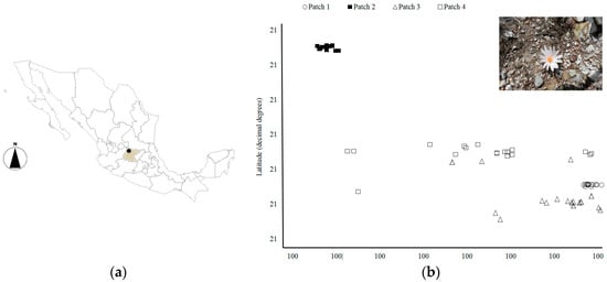
Figure 1.
Location of the study area in the Mexican Republic. In (a) the shaded area indicates the Guanajuato state and the dark point the approximate location of the arid hills occupied by Mammillaria albiflora; in (b) the real geographic distribution of the sampled individuals and the patch in which they were collected is marked with a symbol. The precise geographic coordinates are omitted in the axes due to the critical conservation concern of the species (photo by Sofia Solórzano).
2.2. Sampling Tissue
We collected tissue samples in the total four patches in which M. albiflora lives (Figure 1b). A total of six expeditions were carried out from September 2011 to April 2012, and an additional visit occurred in July 2016. From 20 to 35 different individuals were sampled in each patch, reaching a total of 96 tissue samples (collecting permissions SGPA/DGVS701833/11; SGPA/DGVS/06880/16) of different adult individuals (>1.5 cm in diameter) obtained. For all individuals, geographic coordinates were recorded during the fieldwork. All tissue samples were individually labeled and stored in liquid nitrogen immediately after they were collected.
2.3. Genotyping and Genetic Analyses
To obtain high concentrations of DNA with a quality of 1.80 at an absorbance of 260/280, only the superficial green living tissue (photosynthetic parenchyma) of the stem was collected. All the spines attached to the tissue were mechanically eliminated before starting the DNA isolation protocol. Total genomic DNA was isolated for 70 to 100 mg of the frozen vegetative tissue that was analyzed, according to the instructions of DNAeasy Plant MiniKit (Qiagen, Valencia, CA, USA). The quality of PCR products was not altered if the EB buffer included in this kit was replaced with water pH 8.
The fresh DNA was immediately frozen at −20 °C and an aliquot of 5 μL of each of the 96 samples was charged in horizontal gels of agarose 0.8%, which were run during 30 min at 90 V. They were stained with ethidium bromide and visualized with UV light to visualize the DNA of the samples.
In total, 11 loci of microsatellites were initially assayed using the same PCR conditions described for M. crucigera [37], and later by the specific conditions that were established (Table 1).

Table 1.
Genetic diversity described for M. albiflora based on 10 polymorphic loci and 96 individual samples across four patches. The table indicates the specific alignment temperature for each locus; total number of alleles (NT); the effective number of alleles; the observed heterozygosity (HO) and expected heterozygosity (HE) by locus; inbreeding coefficient (FIS); and the p-value < 0.05 after Bonferroni correction indicates Hardy-Weinberg Disequilibrium.
The PCR reactions were prepared by locus for each of the 96 samples; these were run in the Thermocycler VERITI (Applied Biosystems, Carlsbad, CA, USA). The locus MamVTC14 was discarded by monomorphism across the four patches. The locus MamVTC9 was monomorphic in patch 3, but polymorphic in the rest of the patches, so it was included in the statistical analyses. None locus showed null alleles according to Microchecker analysis [38]. All forward primers of the l0 loci were tagged with NED or FAM fluorochromes (for primers details see [37]). The electrophoresis of the PCR fragments was carried out in the sequencer ABI 3100; the size of the alleles was determined with ROX 500 with the software Gene Mapper (Applied Biosystems).
2.4. Population Structure
For assessing the genetic structure, we based our predictions within the framework of the isolation by distance model and the statistical tests followed the perspective of fine-scale structure analysis recommended for species that occupy small geographic areas [15]. Initially, we searched for population structure applying the ancestry model Admixture implemented in STRUCTURE v.2.3.2 [39]. This model was run assuming allele frequencies correlated, a burning period of 10 and Markov chain Monte Carlo reps of 10,000. The number of K tested was of 1 to 4 with 200 replicates for each one. The value of ΔK was calculated in STRUCTURE HARVESTER [40]. The gene flow (Nm) levels and the coefficient of differentiation were based on 110 permutations and these were calculated as an average among the four patches and paired comparisons between patches using Arlequin V. 3.5 [41]. The spatial autocorrelation genetic analyses were based on 1000 random permutations and were carried out in GenAlEx V.6 [42]. These described the relatedness based on standardized Nei’s genetic distance between the genotypes and their geographical location, which were plotted on the Principal Coordinate Analysis (PCoA); the Mantel test tested the magnitude of the correlations (R2) between the matrices of geographical distance and those of genetic distances of the genotypes. Mantel tests were applied to identify the thresholds geographic distances in which the autocorrelations became statistically significant. The population differentiation (FST) among patches was estimated on pairwise distances that were calculated with the software GDA [43] and plotted as a dendrogram with MEGA 7.0.18 [44]. Finally, the search of genetic barriers to gene flow was carried out with software Barrier 2.2 [45]. To test the robustness of these barriers, a total of 1000 matrices of FST were generated by bootstrapping in MSA [46]. These matrices were run in Barrier 2.2 [45] in order to test the number of matrices that supported each of the barriers identified.
2.5. Genetic Diversity
The statistical analyses were hierarchized by species, patches and locus. The Hardy-Weinberg equilibrium (HWE) and linkage equilibrium (LE) were calculated on the Markovian model with 10,000 steps demorization and a seed of 1,000,000 steps using Arlequin V. 3.5 [41]. The p-values of these estimators were corrected with the Bonferroni test [47]. The allele diversity, the total number of alleles, the number of private alleles, and the effective number of alleles were calculated using the program GDA V.1 [43]. The occurrence of bottleneck was tested with the software Bottleneck 1.2.02 [48], which is based on the mutation models TPM, SMM and IAM. These models were based on 1000 iterations, and their statistical support was according to the sign rank and Wilcoxon tests. Finally, we estimated the past population size using the Tajima’s test based on the mutation model of infinite sites (Θ = 4Neµ, [49]) implemented in Arlequin V. 3.5 [41].
3. Results
3.1. Population Structure
The highest value for ΔK was estimated for K = 2, followed by K = 3 (Figure 2). Clearly the individuals of patch 3 were clustered together, and when K = 3, there is a clearer potential allele migration among different patches according to the geographical origin of the individuals (Figure 1b). The average of the genetic differentiation is significant among the four patches (average FST = 0.17, p < 0.05). The paired comparison showed that only there is no genetic differentiation between patches 1 and 4 (FST = 0.002, p =0.21), whereas the rest of the comparisons between patches were significant (1 vs. 2 (FST = 0.20, p =0.00); 1 vs. 3 (FST = 0.25, p = 0.02); 2 vs. 3 (FST = 0.27, p = 0.01); and 2 vs. 4 (FST = 0.18, p = 0.01)). These levels of genetic differentiation between patches increase when the gene flow reduces (R2 = 0.85, p = 0.005); the gene flow levels between patches decrease as the geographic distance increases (R2 = 0.70, p = 0.001). The Mantel tests showed that the correlations between geographic distances and genotypes’ genetic distances are significant when they are ≥1100 m. The PCoA analysis revealed a distribution of the genotypes distinct to that described by the geographical origin of the individuals (Figure 1b and Figure 3) and showed potential genotype migration according to the geographic distances that separate the patches. Three main genetic neighborhoods are described according to the autocorrelation of the genotypes. Most of the genotypes of the patch 2 are segregated in the axis 1, which also clustered most of the genotypes of patch 3 where 10 individuals had identical genotypes. In the axis 2, genotypes of the patches 1 and 4 are clustered. A total of six genotypes are sparsely distributed. This PCoA analysis separates the genotypes of the patches 2 and 3 (the most geographically distant), and in the dendrogram based on pairwise distances, patch 3 showed the largest genetic distance with respect to the other 3 patches (Figure 4). Additionally, three genetic barriers that restrict the gene flow between the four patches were identified, but these had different robustness. One barrier was supported by 100% of the FST bootstrapped matrices, and the other two by <60% of these matrices (Figure 5).
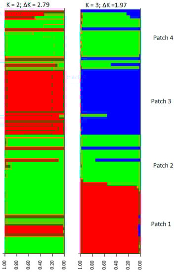
Figure 2.
Genetic structure of the individuals into 2 and 3 genetic groups. The highest value of ΔK is estimated for K = 2. In K = 3, an unweighted pair group method arithmetic average (UPGMA) analysis confirmed the clustering of the individuals of patch 3. Potential migration of alleles among patches is visualized by entire or partial intercalated bars.
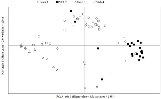
Figure 3.
Genetic relatedness revealed by the spatial analysis of Principal Component Analysis. The two first axes added 60% of the variance that determines the spatial distribution among the genotypes.
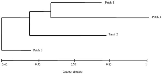
Figure 4.
The cluster that describes the genetic relationships among patches constructed with the UPGMA model.
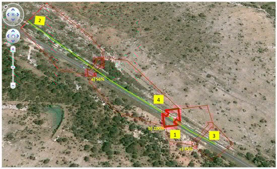
Figure 5.
The three genetic barriers (a, b, c) to gene flow identified among the four patches (1, 2, 3, 4) of M. albiflora are indicated by the rows. The percentage beside each label of the barrier indicates the bootstrapped matrices that support them. The polygon constructed by barrier was drawn on a true image of the study area downloaded on September 2016 with the free application Google Maps. The geographic distance between patch 2 and 3 is of 4.2 km.
3.2. Genetic Diversity
For M. albiflora, the observed heterozygosity (0.33) was lower than the expected one (0.43), and the average inbreeding coefficient over the four patches was significant (FIT = 0.21, p = 0.01). After corrections for multiple comparisons the linkage disequilibrium was detected between locus MamVTC6 and the loci MamVTC7 and MamVTC12; and MamVTC12 to MamVTC7 and MamVTC8. Two loci (MamVTC5 and MamVT7) were in HWE, but the other eight were in HWD (Table 1). The average of inbreeding coefficient (FIS) is significant among patches (FIS = 0.10, p = 0.003), but only patches 3 and 4 have significant values of FIS differing of zero (Table 2). In the 96 samples of M. albiflora, a total of 51 alleles across 10 loci were identified. The allele diversity is low in the four patches and the average number of alleles by locus was five. Although all of them have private alleles (Table 2), they share 84% of the alleles.
Table 2.
Genetic diversity is described by patch based on the observed heterozygosity (HO) and expected heterozygosity (HE), inbreeding coefficient (FIS), the mean number of alleles by locus (NA), and the number of private alleles (AP). SE = Standard Error. In parenthesis are the individuals sampled by patch.
The linkage disequilibrium was estimated in patch 1 between the alleles of MamVTC2 with those of the loci MamVTC6 and MamVTC7. In addition, LD was also estimated between the alleles of MamVTC12 with those of the loci MamVTC8 and MamVTC6 with MamVTC7. The three mutation models did not support the existence of a bottleneck effect in M. albiflora since the p-values for both the sign and Wilcoxon tests were >0.05. Finally, the Tajima model predicted that the population effective size in the past was ~15,114 individuals.
4. Discussion
The hypothesis established in this study about the low allele diversity but relatively high values of heterozygosity is confirmed. The allele variation in a population is strongly influenced by genetic drift, which accelerates the loss of alleles when the effective population size is small. The natural populations can have small effective sizes by the drastic reduction in their size (bottleneck) or by a founder event [10,34,50]. Here, the bottleneck effects were not statistically supported for M. albiflora, but this may be related to the fact that we did not have the 20 sampled loci as the software demands [48]. Another explanation is that in M. albiflora an event of bottleneck effectively occurred but, as has been shown for other species [51], if this was very ancient it could not be detected since the mutation-drift equilibrium was already restored. Also, it may be that the bottleneck has been occurring gradually for a long time in a diffuse mode, which causes a relatively low number of alleles with relatively discordant levels of heterozygosity [52], like the results here obtained. However, the population effective size modeled was nearly 15 times larger than the current total censed population size [32], which suggests decrement in the population size of M. albiflora.
The concern of the low allele variation is that it if continues diminishing, eventually over generations the levels of homozygosity and inbreeding will gradually increase [10,13,50] by the fact that the current population has a small population size, a situation that could increase the extinction risk in M. albiflora.
Respect to the levels of genetic diversity evaluated in other nine endemic Mammillaria species M. albiflora has the lowest values of genetic diversity (Table S1 of Supplementary File). Although the number of individuals, populations and microsatellite loci sampled influences the descriptors of the genetic diversity [16], it is evident that M. albiflora did not increase its genetic diversity, though it had more sampling than in M. hernandezii and M. zephyranthoides. These 10 compared species are of conservation concern by their low population densities and by their restricted distribution range, but M. albiflora is the species with the smallest geographic range [32], and this factor may be considered a key criterion in a conservation plan to protect this species and its habitats.
In relation to the second hypothesis related to genetic differentiation, the results obtained for M. albiflora were unexpected, since they do not represent the general pattern predicted for the species of restricted distribution [9] and even less for the ENEs of small population size, like M. albiflora. This strong differentiation of M. albiflora adjusted to isolation by distance model; however, the fact that we had only four points (patches) for the statistical analyses suggest caution. Other Mammillaria species also adjusted to this model [20], but other did not [20,25], which point out that not all the species of narrow/restricted range will have gene flow patterns predicted by this model. We consider that the genetic structure of this species is caused by the poor dispersion of seeds and pollen previously documented [32]. Consequently, the individuals of the four patches are segregating in very small areas founding genetic neighborhoods. It seems that the movement of the alleles is limited by three genetic barriers that might be represented in (1) the highway that has been isolating patch 1 from the other ones; (2) though the patches 2, 3 and 4 are located on the same side of the highway and they are not geographically separated, the barrier is the severe land transformation that has caused unsuitable habitats, in which the seed germination and seedling establishment probably cannot occur; (3) we interpreted the third genetic barrier in the small but dense aggregations of arboreous vegetation causing a shading microenvironment, in which no individuals of M. albiflora are present.
In addition, other process involved in the genetic population subdivision is genetic drift, which may be promoting the genetic structuring, since it increases the variances of the allelic frequencies inversely to the population size (σ2 = poqo/2N; confirm [10]). Thus, our results indicate that the isolation by distance model is appropriate for explaining the genetic structure levels of the ENEs, such as M. albiflora, and this theoretical platform also allows inferring evolutionary and ecological processes that are occurring in them.
According to the results of the genetic structure, patches 1 and 2 are the most genetically differentiated and these should be considered for conservation issues. The number of private alleles also addressed the patch 2 for conservation concern. In fact, patch 1 is the only one that is in the other side of the highway. It seems that patch 2 is increasing in genetic differentiation and it potentially receives migrants of patch 4, whose genotypes are also represented in patch 1. The land (0.04 km2) of patch 3 represents the only area advocated to protect this species but here the high adults harvesting is also documented [32], and the individuals from this patch tend to cluster, while alleles from this area are also potentially migrating to the other patches. However, patch 1 is private land, and deserves government intervention with the land owner for rescuing this area. Then, in order to accelerate the conservation of M. albiflora, firstly it is necessary to undertake a legal protection of patches 2 and 3 that are not private lands. The second action should be to formally list the species in the Mexican National Species Red List in the category of risk of extinction. The third action should maintain M. albiflora in the red list of IUCN, in the category of critically endangered, as is already classified [29]. Finally, the last recommendation is to start a program for promoting the legal in vitro propagation of M. albiflora, as a strategy for reducing its illegal harvesting from its natural habitats. The latter has been already proposed to rescue the ENEs with extremely small population sizes, and often these programs also include the conservation of seeds [4].
Supplementary Materials
The following are available online at www.mdpi.com/1424-2818/8/4/31/s1. Table S1: Comparison of the genetic diversity levels (heterozygosity and allele richness) of M. albiflora and other Mammillaria species (in parenthesis the number of the reference cited in literature). N = total of the sampled individuals; n = number of subpopulations sampled; L = number of polymorphic loci sampled. HO = the observed heterozygosity for the species level (the mean based on the total of the subpopulations analyzed and in the total of the loci used); HE = the expected heterozygosity for the species, NT = the total number of alleles accounted in all loci sampled, NA = the mean number of alleles by locus.
Acknowledgments
This research was supported by the Programa UNAM-DGAPA-PAPIIT (IN220711). We appreciate the help of Emilio Brito for helping in the prospection visits to the study area. We also thank Federico Gama, Head of NGO Can-Te A. C., who allowed the sampling in this land. Thank Cruz-Santos by the 37 individuals amplified with 1–3 loci. The comments of two anonymous reviewers and editor improved the quality of this manuscript. The non-tagged primers were produced at IBT-UNAM (P. Gaytán and Eugenio López). The electrophoresis of the fragments was kindly provided by Laura Márquez Valdelamar, IB-UNAM.
Author Contributions
This study is part of a research projected led by Sofia Solórzano, in which Patricia Dávila and Salvador Arias were collaborators. Sofia Solórzano conducted the field and molecular sampling. Sofia Solórzano and Patricia Dávila obtained the sampling permissions. Sofia Solórzano, Patricia Dávila and Salvador Arias wrote this manuscript.
Conflicts of Interest
The authors declare no conflict of interest. The founding sponsor had not role in the design of the study, in the sampling, analyses, or interpretation of data; in writing of the manuscript, and in the decision to publish the results.
References
- Rabinowitz, D. Seven forms of rarity. In The Biological Aspects of Rare Plant Conservation; Synge, H., Ed.; John Wiley & Sons: New York, NY, USA, 1981; pp. 205–217. [Google Scholar]
- Kunin, W.E.; Gaston, K.J. The biology of rarity: Patterns, causes and consequences. Trends Ecol. Evol. 1993, 8, 298–301. [Google Scholar] [CrossRef]
- Callmander, M.W.; Schatz, G.E.; Lowry, P.P. IUCN Red List Assessment and the Global Strategy for Plant Conservation: Taxonomists must act now. Taxon 2005, 54, 1047–1054. [Google Scholar] [CrossRef]
- Ma, Y.; Chen, G.; Grumbine, R.E.; Dao, Z.; Sun, W.; Guo, H. Conserving plant species with extremely small populations (PSESP) in China. Biodivers. Conserv. 2013, 22, 803–809. [Google Scholar] [CrossRef]
- International Union for Conservation of the Nature (IUCN). IUCN Red List Categories and Criteria. Available online: http://www.iucnredlist.org/static/categories_criteria_3_1 (accessed on 11 September 2016).
- López-Pujol, J.; Martinell, M.C.; Massó, S.; Blanché, C.; Sáez, L. The “paradigm of extremes”: Extremely low genetic diversity in an extremely narrow endemic species, Coristospermum huteri (Umbelliferae). Plant Syst. Evol. 2013, 299, 439–446. [Google Scholar] [CrossRef]
- Coates, D.J.; Carstairs, S.; Hamley, V.L. Evolutionary patterns and genetic structure in localized and widespread species in the Stylidium caricifolium complex (Stylidiaceae). Am. J. Bot. 2003, 90, 997–1008. [Google Scholar] [CrossRef] [PubMed]
- Wulff, A.S.; Hollingsworth, P.M.; Ahrends, A.; Jaffré, T.; Veillon, J.M.; L’Huillier, L.; Fogliani, B. Conservation Priorities in a Biodiversity Hotspot: Analysis of narrow endemic plant species in New Caledonia. PLoS ONE 2013, 8. [Google Scholar] [CrossRef] [PubMed]
- Hamrick, J.L.; Godt, M.J. Allozyme diversity in plant species. In Plant Population Genetics, Breeding and Genetic Resources; Brown, A.H.D., Clegg, M.T., Kahler, A.L., Weir, B.S., Eds.; Sinauer Associates: Sunderland, MA, USA, 1989; pp. 43–63. [Google Scholar]
- Frankham, R.; Ballou, J.D.; Briscoe, D.A. Introduction to Conservation Genetics; Cambridge University Press: Cambridge, UK, 2002. [Google Scholar]
- Rymer, P.D.; Morris, E.C.; Richardson, B.J. Breeding system and population genetics of the vulnerable plant Dillwynia tenuifolia (Fabaceae). Austral Ecol. 2002, 27, 241–248. [Google Scholar] [CrossRef]
- Godt, M.J.W.; Caplow, F.; Hamrick, J.L. Allozyme diversity in the federally threatened golden paintbrush, Castilleya levisecta (Scrophulariaceae). Conserv. Genet. 2005, 6, 87–99. [Google Scholar] [CrossRef]
- Templeton, A.R.; Read, B. Inbreeding: One word, several meanings, much confusion. In Conservation Genetics; Loeschke, J.T., Jain, S.K., Eds.; Birkhäuser Verlag: Basel, Switzerland, 1994; pp. 91–105. [Google Scholar]
- Clarke, L.J.; Jardine, D.I.; Byrne, M.; Shepherd, K.; Lowe, A.J. Significant population genetic structure detected for a new and highly restricted species of Atriplex (Chenopodiaceae) from Western Australia, and implications for conservation management. Aust. J. Bot. 2012, 60, 32–41. [Google Scholar] [CrossRef]
- Vekemans, X.; Hardy, O. New insights from fine-scale spatial genetic structure analyses in plant populations. Mol. Ecol. 2004, 13, 921–935. [Google Scholar] [CrossRef] [PubMed]
- Nybom, H. Comparison of different nuclear DNA markers for estimating intraspecific genetic diversity in plants. Mol. Ecol. 2004, 13, 1143–1155. [Google Scholar] [CrossRef] [PubMed]
- Karron, J.D.; Linhart, Y.B.; Chaulk, C.A.; Robertson, C.A. Genetic structure of populations of geographically restricted and widespread species of Astragalus (Fabaceae). Am. J. Bot. 1988, 75, 1114–1119. [Google Scholar] [CrossRef]
- Filippov, E.G.; Andronova, E.V. Genetic differentiation in plants of the genus Cypripedium from Russia inferred from allozyme data. Genetika 2011, 47, 615–623. [Google Scholar] [CrossRef] [PubMed]
- Nicolè, F.; Tellier, F.; Vivat, A.; Till-Bottraud, I. Conservation unit status inferred for plants by combining interspecific crosses and AFLP. Conserv. Genet. 2007, 8, 1273–1285. [Google Scholar] [CrossRef]
- Solórzano, S.; Dávila, P. Identification of conservation units of Mammillaria crucigera (Cactaceae): Perspectives for the conservation of rare species. Plant Ecol. Divers. 2005, 8, 559–569. [Google Scholar] [CrossRef]
- Gibson, A.C.; Nobel, P.S. The Cactus Primer; Harvard University Press: Cambridge, MA, USA, 1986. [Google Scholar]
- Arias-Montes, S.; Gama-López, S.; Guzmán-Cruz, L.U. Cactaceae, A.L. Juss. In Flora del Valle de Tehuacán-Cuicatlán; Fascículo 14; Universidad Nacional Autónoma de México: Mexico City, Mexico, 1997. (In Spanish) [Google Scholar]
- International Union for Conservation of the Nature (IUCN). The IUCN Red List of Threatened Species. Available online: http://www.iucnredlist.org/ (accessed on 7 October 2016).
- Guzmán-Cruz, L.U.; Arias-Montes, S.; Dávila, P. Catálogo de Cactáceas Mexicanas; Universidad Nacional Autónoma de México, Comisión Nacional para el Conocimiento y Uso de la Biodiversidad: Distrito Federal, Mexico, 2007. (In Spanish) [Google Scholar]
- Solórzano, S.; Cuevas-Alducin, P.D.; Gómez-García, V.; Dávila, P. Genetic diversity and conservation of Mammillaria huitzilopochtli and M. supertexta, two threatened species endemic of the semiarid region of central Mexico. Rev. Mex. Biodivers. 2014, 85, 565–575. [Google Scholar] [CrossRef]
- Solórzano, S.; Téllez, O.; Álvarez-Espino, R.; Dávila, P. Unidades genéticas para la conservación de Mammillaria (Cactaceae). Fitotecnica 2016. under review (In Spanish) [Google Scholar]
- Macías-Arrastio, F.F. Diversidad y Estructura Genética Poblacional de Mammillaria solisioides Backeb. Especie Endémica de la Mixteca de Oaxaca y Puebla. Bachelor Thesis, Universidad Nacional Autónoma de México, Mexico City, Mexico, 21 March 2014. [Google Scholar]
- Cruz-Santos, A. Evaluación de la Diversidad Genética Poblacional de Mammillaria albiflora (Cactaceae): Especie Endémica del Estado de Guanajuato, México. Bachelor Thesis, Universidad Nacional Autónoma de México, Mexico City, Mexico, 8 April 2015. [Google Scholar]
- Quezada-Ramírez, S. Análisis de la Diversidad Genética de Mammillaria rekoi Britton & Rose (Cactaceae: Especie Endémica del Estado de Guanajuato, México. Bachelor Thesis, Universidad Nacional Autónoma de México, Mexico City, Mexico, 1 April 2016. [Google Scholar]
- López-Ortiz, N.M. Diversidad y Estructura Genética Poblacional de Mammillaria zephyranthoides (Cactaceae): Una Especie Endémica de México. Bachelor Thesis, Universidad Nacional Autónoma de México, Mexico City, Mexico, 24 January 2014. [Google Scholar]
- Fitz Maurice, B.; Fitz Maurice, W.A.; Sánchez, E.; Guadalupe-Martínez, J.; Bárcenas-Luna, R. Mammillaria albiflora. In The IUCN Red List of Threatened Species 2013: e.T40824A2934715; IUCN Global Species Programme Red List Unit: Cambridge, UK, 2013; Available online: http://dx.doi.org/10.2305/IUCN.UK.2013-1.RLTS.T40824A2934715.en (accessed on 8 August 2016).
- Solórzano, S.; Téllez, O; Arias, S.; Dávila, P. The ecologic evaluation of the conservation status of Mammillaria albifora (Cactaceae). in preparation.
- Frankham, R. Relationships of genetic variation to population size in wildlife. Conserv. Biol. 1996, 10, 1500–1508. [Google Scholar] [CrossRef]
- Karron, J.D. Patterns of genetic variation and breeding systems in rare plants species. In Genetics and Conservation of Rare Plants; Falk, D.A., Holsinger, K.E., Eds.; Oxford University Press: New York, NY, USA, 1991; pp. 87–98. [Google Scholar]
- Comisión Nacional del Agua (CNA). Databases. 2016. Available online: http://smn.cna.gob.mx (accessed on 23 September 2016). (In Spanish)
- Zamudio, S. Diversidad de ecosistemas del Estado de Guanajuato. In La Biodiversidad en Guanajuato: Estudio de Estado; Comisión Nacional para el Conocimiento y Uso de la Biodiversidad (Conabio)/Instituto de Ecología del Estado de Guanajuato (IEE): Mexico City, Mexico, 2012; Volume II, pp. 21–55. (In Spanish) [Google Scholar]
- Solórzano, S.; Cortés-Palomec, A.C.; Ibarra, A.; Dávila, P.; Oyama, K. Isolation, characterization and cross-amplification of polymorphic microsatellite loci in the threatened endemic Mammillaria crucigera. Mol. Ecol. Res. 2009, 9, 156–158. [Google Scholar] [CrossRef] [PubMed]
- Van Oosterhout, C.; Hutchinson, B.; Wills, D.; Shipley, P. Microchecker: Software for identifying and correcting genotyping errors in microsatellite data. Mol. Ecol. Res. 2004, 4, 535–538. [Google Scholar]
- Pritchard, J.A.; Stephens, M.; Donnelly, P. Inference of Population Structure Using Multilocus Genotype Data. Genetics 2000, 155, 945–959. [Google Scholar] [PubMed]
- Earl, D.A.; von Holdt, B.M. STRUCTURE HARVESTER: A website and program for visualizing STRUCTURE output and implementing the Evanno method. Conserv. Genet. Res. 2012, 4, 359–361. [Google Scholar] [CrossRef]
- Excoffier, L.; Lischer, H.E.L. Arlequin suite ver 3.5: A new series of programs to perform population genetics analyses under Linux and Windows. Mol. Ecol. Res. 2010, 10, 564–567. [Google Scholar] [CrossRef] [PubMed]
- Peakall, R.; Smouse, P.E. GenAlEx V.6, Genetic Analysis in Excel. Population Genetic Software for Teaching and Research. The Australian National University: Canberra, Australia, 2015. Available online: http://www.anu.edu.au/BoZo/GenAlEx/ (accessed on 6 September 2016).
- Lewis, P.; Zaykin, D. Genetic Data Analysis: Computer Program for the Analysis of Allelic Data. 2001. Available online: http://lewis.eeb.uconn.edu/lewishome/software.html (accessed on 12 October 2016).
- Tamura, K.; Stecher, G.; Kumar, S. MEGA 7.0.18. Molecular Evolutionary Genetics Analysis. 1993–2016. Available online: http://www.megasoftware.net/home (accessed on 4 April 2015).
- Dieringer, D.; Schlötterer, C. Microsatellite Analyser (MSA): A platform independent analysis tool for large microsatellite data sets. Mol. Ecol. Resour. 2003, 3, 167–169. [Google Scholar] [CrossRef]
- Manni, F.; Guérard, E.; Heyer, E. Geographic patterns of (genetic, morphologic, linguistic) variation: How barriers can be detected by “Monmonier’s algorithm”. Hum. Biol. 2004, 76, 173–190. [Google Scholar] [CrossRef] [PubMed]
- Sokal, R.R.; Rohlf, J.L. Biometry, 3rd ed.; Freeman: New York, NY, USA, 1995. [Google Scholar]
- Cornuet, J.M.; Luikart, G. Description and power analysis of two tests for detecting recent population bottlenecks from allele frequency data. Genetics 1996, 144, 2001–2014. [Google Scholar] [PubMed]
- Tajima, F. The effect of change in population size on DNA polymorphism. Genetics 1989, 123, 597–601. [Google Scholar] [PubMed]
- Frankham, R. Conservation genetics. Annu. Rev. Genet. 1995, 29, 305–327. [Google Scholar] [CrossRef] [PubMed]
- Nikolic, N.; Chevalet, C. Detecting past changes of effective population size. Evol. Appl. 2014, 7, 663–681. [Google Scholar] [CrossRef] [PubMed]
- Allendorf, F.W. Genetic drift and the loss of the alleles versus heterozygosity. Zoo Biol. 1986, 5, 181–190. [Google Scholar] [CrossRef]
© 2016 by the authors; licensee MDPI, Basel, Switzerland. This article is an open access article distributed under the terms and conditions of the Creative Commons Attribution (CC-BY) license (http://creativecommons.org/licenses/by/4.0/).