Genotyping-By-Sequencing for Plant Genetic Diversity Analysis: A Lab Guide for SNP Genotyping

Abstract

Genotyping-by-sequencing (GBS) has recently emerged as a promising genomic approach for exploring plant genetic diversity on a genome-wide scale. However, many uncertainties and challenges remain in the application of GBS, particularly in non-model species. Here, we present a GBS protocol we developed and use for plant genetic diversity analysis. It uses two restriction enzymes to reduce genome complexity, applies Illumina multiplexing indexes for barcoding and has a custom bioinformatics pipeline for genotyping. This genetic diversity-focused GBS (gd-GBS) protocol can serve as an easy-to-follow lab guide to assist a researcher through every step of a GBS application with five main components: sample preparation, library assembly, sequencing, SNP calling and diversity analysis. Specifically, in this presentation, we provide a brief overview of the GBS approach, describe the gd-GBS procedures, illustrate it with an application to analyze genetic diversity in 20 flax (Linum usitatissimum L.) accessions and discuss related issues in GBS application. Following these lab bench procedures and using the custom bioinformatics pipeline, one could generate genome-wide SNP genotype data for a conventional genetic diversity analysis of a non-model plant species.

1. Introduction

Plant genetic diversity analysis is an important component in studies of plant genetics, breeding, conservation and evolution. Such analysis, however, depends on genome sampling with sufficient and informative genetic markers, such as single nucleotide polymorphism (SNP), and many species of interest are lacking SNP markers. Efforts have been made to develop SNP markers through various approaches, such as chip hybridization or targeting-specific genomic regions [1]. However, such efforts are expensive and labour intensive, as it is technically difficult to develop SNP markers for plant species. Plants usually have large complex genomes with abundant sequence repeats and genome duplications. Furthermore, many species do not have sequenced genomes and are considered to be non-model plants, making the SNP discovery more challenging.

Genotyping-by-sequencing (GBS) has recently emerged as a promising genomic approach for exploring plant genetic diversity on a genome-wide scale [2,3,4,5,6], thanks to the advances in next generation sequencing (NGS) technologies [7,8]. The GBS approach is based on genome reduction with restriction enzymes [9], does not require a reference genome for SNP discovery, is a combined one-step process of marker discovery and genotyping and provides a rapid, high-throughput and cost-effective tool for a genome-wide analysis of genetic diversity for a range of non-model species and germplasm sets [5,10]. These characteristics are advantageous and encouraging for genetic diversity analysis of plants with no informative markers available. The GBS application is more appealing for exploring useful genetic diversity in ex situ plant germplasm, particularly considering 7.4 million accessions of several thousands of non-model species that are conserved worldwide [11].

Despite this promising potential, GBS has not been widely applied to analyze plant genetic diversity as yet, and its application still faces many uncertainties and challenges. GBS is still evolving to address many key technical issues. Robust protocols have been advanced to increase genome coverage; new bioinformatics pipelines have been developed for SNP discovery and genotyping; and effective imputations for missing data have been proposed. These developments have provided more choice in GBS application. Furthermore, the current GBS approach has been developed largely based on model plants (i.e., those species with sequenced genomes), but plant genetic diversity analyses have their focus more toward non-model plants. Existing bioinformatics pipelines need to be modified for generating de novo contigs to be used as a reference for SNP discovery and genotyping. Moreover, GBS is conceptually simple, but in practice involves many steps using a range of molecular biology skills and requiring bioinformatics analyses. An easy-to-follow tool for its application is desired, but largely lacking, for researchers with little experience in NGS research and bioinformatics analysis.

Here, we present a genetic diversity-focused GBS (gd-GBS) protocol that we have developed and are currently using to analyze plant genetic diversity. Our presentation can serve as both an introduction to GBS and as an easy-to-follow lab guide to assist a researcher through sample preparation, library assembly, sequencing and extraction of SNPs from high-throughput data for genetic diversity analysis. Specifically, in this presentation, we provide a brief overview of the GBS approach, describe the gd-GBS procedures, illustrate it with an application to analyze genetic diversity in 20 flax (Linum usitatissimum L.) accessions and discuss related issues in GBS application. It is our hope that researchers can start to take advantage of the power of whole genome sequencing to analyze genetic diversity, particularly in non-model plants, with the help of the published gd-GBS protocol.

2. An Overview of the GBS Approach

GBS was first coined by Rob Elshire and his colleagues as a simple highly-multiplexed system for constructing reduced representation libraries for the Illumina NGS platform [3]. It was inspired by the whole genome sequence effort in rice [2] and builds upon the protocol of restriction site-associated DNA (RAD) tags [12]. Elshire’s system employed the Illumina platform and was equipped with a bioinformatics pipeline for SNP discovery and genotyping. This system can generate a large number of genotyped SNP markers for use in genetic analyses and has been successfully tested on many organisms. However, Elshire’s GBS protocol is not unique, and many similar GBS protocols were also developed following the same idea of genomic reduction [9] and taking advantage of NGS technology [13,14,15,16]. For example, we also developed a similar GBS protocol using the Roche 454 pyrosequencing platform that was capable of generating thousands of genotyped SNP markers specifically for plant genetic diversity analysis [4,10,17].

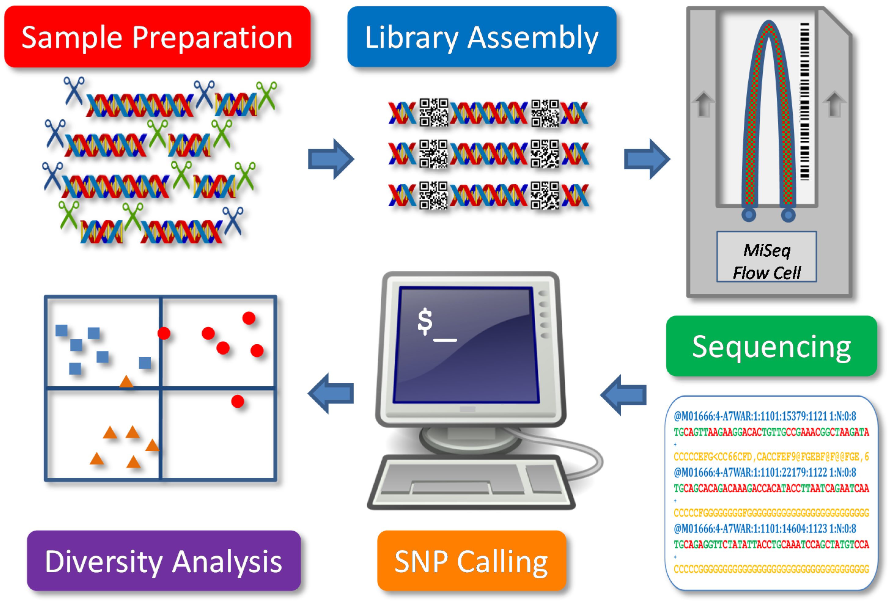
In general, GBS can be regarded as one of several reduced-representation sequencing methods for genotyping. As illustrated in Figure 1, it involves five major components: sample preparation, library assembly, sequencing, SNP calling and diversity analysis. Major steps include DNA extraction and digestion, adapter ligation, PCR amplification, fragment size selection, library pooling, sequencing, data processing, SNP calling and genetic diversity analysis. These steps may vary in restriction endonuclease (RE) use, NGS platform and in bioinformatics analysis for SNP genotyping for different study objectives. The application of GBS for genetic diversity analysis, for example, focuses on genome-wide sampling of a large number of samples, while other genetic analyses, such as genome-wide association studies (GWAS), emphasize the accuracy of SNP calling with read depth to reveal genic signals. Specifically, an informative genetic diversity analysis requires SNP data with large genome coverage, high genotyping accuracy, more balanced observation and less bias, which may be technically introduced from sequence mapping, heterozygote detection and data filtering.

The GBS approach has several major features in favour of plant genetic diversity analysis. First, it combines the processes of marker discovery and genotyping and provides a rapid, high throughput and cost-effective tool for a genome-wide analysis of genetic diversity [5,10]. Second, it requires no prior sequencing of the plant genome and provides direct genotyping of plants with complex genomes without prior SNP discovery, making the approach more accessible to non-model species. Third, and most importantly, it generates a large number of genome-wide SNP data, allowing for better genome sampling. Despite its benefits, the GBS approach also displays some limitations: (1) the presence of large amounts of missing data [4,10,17,18,19] largely due to the use of low coverage sequencing [20]; and (2) uneven genome coverage [21], due to the use of REs and fragment size selection.

Figure 1. Schematic presentation of a genotype-by-sequencing application for plant genetic diversity analysis. Five components are illustrated.

Figure 1. Schematic presentation of a genotype-by-sequencing application for plant genetic diversity analysis. Five components are illustrated.

Figure 2. Flow chart of the genetic diversity-focused genotyping-by-sequencing (gd-GBS) protocol. The gd-GBS protocol consists of five major parts and many steps. Each part (filled box) relates back to the components in Figure 1. Arranged in columns beneath each part are the ordered major steps in outlined boxes of the same colour. Bracketed terms refer to specific equipment, reagents, kits or software used.

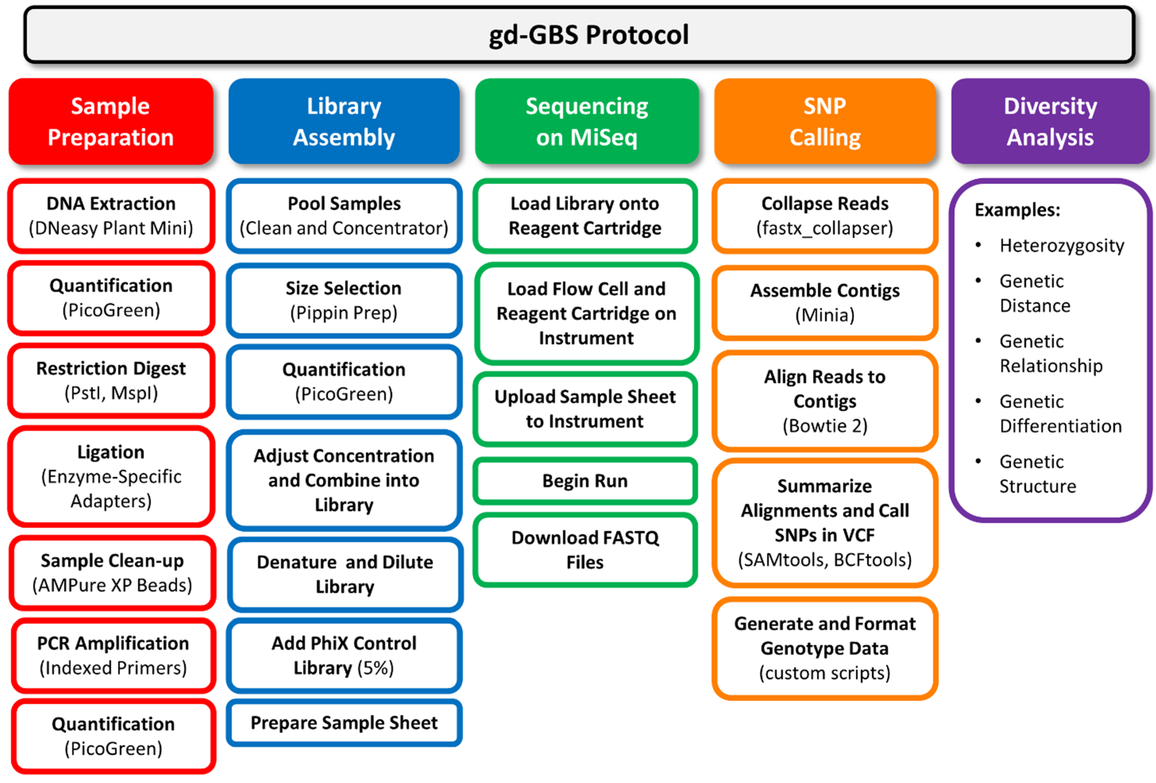
Figure 2. Flow chart of the genetic diversity-focused genotyping-by-sequencing (gd-GBS) protocol. The gd-GBS protocol consists of five major parts and many steps. Each part (filled box) relates back to the components in Figure 1. Arranged in columns beneath each part are the ordered major steps in outlined boxes of the same colour. Bracketed terms refer to specific equipment, reagents, kits or software used.

3. The gd-GBS Protocol

Since 2009, we have explored workable GBS protocols for plant genetic diversity analysis based on the Roche 454 pyrosequencing platform [4,10,17] and Illumina HiSeq and MiSeq sequencing platforms. Our new Illumina-based GBS protocol, named “gd-GBS” to distinguish it from others, yields more SNP genotype data with fewer missing observations than those based on the Roche 454 platform. The major features of gd-GBS are the use of two restriction enzymes to reduce genome complexity, the application of Illumina multiplexing indexes for barcoding and the availability of a custom bioinformatics pipeline for genotyping a diploid species. Specifically, gd-GBS has the same five major components as in others’ methods, shown in Figure 1, with major steps illustrated in Figure 2. The complete gd-GBS protocol, including the bioinformatics pipeline “npGeno” (short for non-model plant genotyping), is provided in the online supporting materials. The use of our GBS protocol assumes a researcher: (1) has general knowledge of plant genetic diversity analysis; (2) has a specific genetic diversity project in mind to pursue; (3) has the plant materials prepared and ready to assay; and (4) can access computing resources, such as a Linux server, and has basic operational skills in a Unix environment.

3.1. Part I: Sample Preparation

Total genomic DNA (gDNA) is extracted from ground, freeze-dried, young leaf tissue and quantified. Restriction enzymes PstI and MspI are used to digest gDNA, and the resulting fragments are directly ligated to a pair of enzyme-specific adapters, applied universally to all samples, consisting of a partially sequence-divergent (i.e., “Y” or forked) MspI-specific “Adapter 1” and a fully complementary PstI-specific “Adapter 2” (Table S1). Both adapters contain specific priming sites for the Illumina MiSeq sequencing chemistry (Figure S1). Since the PstI enzyme cannot be heat inactivated, both adapters were designed not to recreate the restriction sites, allowing for ligation at room temperature directly after digestion. The resulting ligated fragments are cleaned to remove any unincorporated adapters and remaining active enzymes. The resulting population of fragments consist of the Adapter 1/Adapter 2 fragments along with the undesirable Adapter 1/Adapter 1 and Adapter 2/Adapter 2 fragments.

Following ligation, the fragments are PCR amplified with primers that are specific to each adapter (Table S1) and consist of an Illumina index sequence (Table S2) and flow cell annealing (FCA) complementary sequences. The combination of the ligated adapters and the PCR primer sequences forms the “full-length adapter” sequences required by the MiSeq instrument. During the first round of PCR, the Adapter 1 priming site is not present due to the divergent “Y” sequence. Thus, any Adapter 1/Adapter 1 fragments cannot be amplified. The Adapter 2-specific primer will bind to the fragment, resulting in the synthesis of the complementary sequence for Adapter 1 for the subsequent rounds of PCR (Figure S1). Adapter 2/Adapter 2 fragments will be amplified, but are relatively rare in the total population, owing to the infrequently cutting PstI enzyme. Additionally, these fragments tend to be larger than the window used for size selection and are filtered out. Elshire et al. [3] observed that Adapter 2/Adapter 2 fragments sequenced inefficiently and did not impact the overall sequence yield. Once PCR is complete, the indexed amplicons are quantified.

3.2. Part II: Library Assembly

Library assembly begins with the pooling of up to four amplicons with similar concentrations. The Pippin Prep (Sage Science, Beverly, MA, USA) electrophoresis instrument is used for the fractionation selection of amplicons between 400 bp and 600 bp, which consist of 260 bp to 460 bp of original gDNA and 140 bp of Illumina-specific sequences in the full-length adapters. During the first several runs of the protocol, particularly when working with a new species, it is beneficial to determine the size range of the fragments generated by PCR prior to pooling and size selection using a microfluidic analyzer, such as the Bioanalyzer (Agilent, Santa Clara, CA, USA) or Experion (Bio-Rad, Hercules, CA, USA) and to evaluate the amount of the fragments that fall within the selected size range.

Size-selected pooled fragments are quantified, and concentrations are adjusted preferentially to 4 nM and combined to form the sample library. Immediately prior to the sequencing run, the sample library is denatured and diluted to 8 pM according to the Illumina MiSeq protocol [22]. To create the final library, a final volume of 5% denatured PhiX Control Library (Illumina, San Diego, CA, USA) is added to the sample library as a spiked-in control and to increase sample diversity to avoid phasing read errors. A MiSeq sample sheet for the library is required for running the MiSeq instrument, and it consists of the names and index sequences associated with each sample in the library and the adapter sequences.

3.3. Part III: Sequencing on MiSeq

The gd-GBS protocol uses the MiSeq “Generate FASTQ” workflow, the “FASTQ Only” application and “TruSeq HT” assay to generate a de-multiplexed set of FASTQ files with the adapter sequences removed upon completion of the sequencing run. The freshly denatured and diluted library containing PhiX is loaded onto a MiSeq Reagent Kit v3 600-cycle cartridge. The run is initiated and monitored according to the protocol outlined by Illumina [23] for the MiSeq instrument. A MiSeq run typically lasts up to 48 h, and the run data, including the FASTQ files, are downloaded. Each sample has two FASTQ files representing the forward and reverse sequencing reads labelled with the respective terms “R1” and “R2”.

3.4. Part IV: SNP Calling

A computational pipeline, npGeno, was specifically developed for SNP discovery and genotyping from FASTQ files (Figure S3). The script npGeno.sh consists of four shell scripts that automate freely available software and custom Perl scripts. The first constructs contigs from sequence reads from all samples, and the second calls SNPs using the constructed contigs as a reference. The third filters resulting SNPs, and the fourth formats data outputs. To construct contigs, fastx_collapser, part of FASTX tools [24], is used to collapse all identical reads down to single unique sequences. Minia software [25,26] is used to construct the de novo reference contigs for calling SNPs. Bowtie 2 [27] is employed to map the reads from each sample against the reference contigs. SAMtools [28] is used to create a pile-up file summary of the aligned reads relative to the contigs, and BCFtools calls SNPs in a variant call format (VCF) file. Custom Perl scripts are developed to create tab-delimited genotype and haplotype data from VCF files, to remove duplicates and missing data and to re-format output data required for various diversity analyses.

The pipeline takes FASTQ input, along with three other input files, and outputs seven data files (Figure S3). It was developed for use on a Linux operating system, as it is dependent on a number of freely available programs. These programs need to be installed in Linux, including setting their proper execution paths, following their respective documented installation instructions.

3.5. Part V: Conventional Genetic Diversity Analysis

Six output data files generated from the pipeline can be used for a genetic diversity analysis. All_SNP_Genotypes.txt and its corresponding haplotype data All_SNP_hap.txt contain all of the genotype and unphased haplotype data obtained for each sample on all of the reference contigs. Clean_SNP_Genotypes.txt and Clean_SNP_hap.txt are the cleaned data after removing loci that show the same genotypes for all of the samples, have missing observations at zero (default) or a higher level or reside within the first and last 20 base pairs (default) of a reference contig. Two extra formatted datasets, Clean_genotype_STRUCTURE.txt and Clean_haplotype_MEGA.txt, can be used by other software, such as PGDSpider [29], to convert them into different formats required for specific diversity analyses. Using the cleaned data, one could perform a conventional genetic diversity analysis of assayed samples to estimate heterozygosity, infer genetic relationships and structure, or quantify genetic distance and differentiation, using commonly applied population genetic analysis tools, such as GenAlEx, AMOVA, STRUCTURE or R packages, according to the study objectives.

4. An Illustration of the gd-GBS Application with Flax

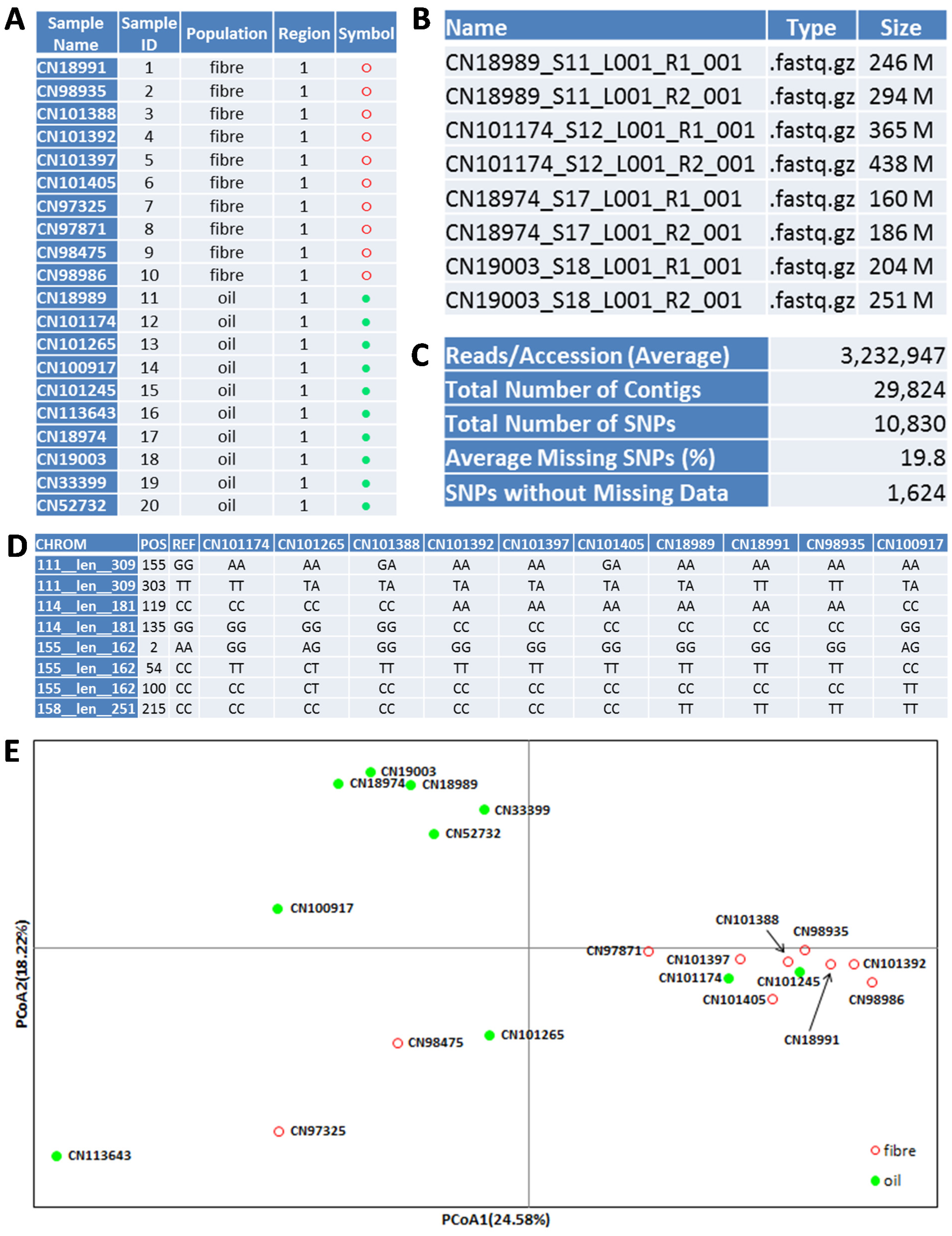
To further illustrate gd-GBS procedures, we present a gd-GBS application in flax. Ten oilseed and 10 fibre flax accessions (Figure 3A) were selected from the flax germplasm collection held at Plant Gene Resources of Canada, Saskatoon, SK, Canada. Seeds were randomly selected from each accession and grown for three weeks in a greenhouse. An individual seedling was randomly selected from each accession, and its leaf tissue was collected, freeze-dried and stored at −20 °C until extracted. Total genomic DNA was extracted using DNeasy Plant Mini Kit (Qiagen, Mississauga, ON, Canada) from 20 mg of powdered leaf tissue. DNA quality was assessed by a 260/280-nm ratio from the Thermo Scientific Nanodrop 8000, and DNA was quantified using the Invitrogen Quant-iT^TM PicoGreen^® dsDNA assay kit (Life Technologies, Burlington, ON, Canada) and adjusted to 20 ng/µL with water.

Restriction enzymes PstI and MspI (New England Biolabs, Whitby, ON, Canada) were selected based on Poland et al. [14], and 200 ng of DNA were digested using Cut Smart Buffer for 3 h at 37 °C. Adapters were designed based on Peterson et al. [13], each containing priming and ligating sites. While the PstI Adapter 2 was a standard double-stranded molecule, the MspI Adapter 1 was a “Y” adapter to prevent the amplification of Adapter 1/Adapter 1 fragments during the PCR (Figure S1). We chose to design adapters without in-line barcodes and instead relied upon Illumina multiplexing indexes designed into the PCR primers (Table S1), allowing the adapters to be universally applied to all samples. Adapters were ligated onto restriction fragments using Invitrogen T4 DNA Ligase (Life Technologies, Burlington, ON, Canada) at 23 °C for 2 h, heat killed at 65 °C for 10 min and stored at −20 °C overnight. The ligation was cleaned to remove unligated adapters using Agencourt^® AMPure^® XP beads (Beckman Coulter, Brea, CA, USA).

Figure 3. An illustration of 20 flax samples (A) and their GBS application outputs: FASTQ file names and sizes (B), major bioinformatics analysis outcomes (C), SNP genotypes (D) and a PCoA plot for sample association (E). Note that (B) and (D) only show a sample of all files and genotypes.

Figure 3. An illustration of 20 flax samples (A) and their GBS application outputs: FASTQ file names and sizes (B), major bioinformatics analysis outcomes (C), SNP genotypes (D) and a PCoA plot for sample association (E). Note that (B) and (D) only show a sample of all files and genotypes.

PCR primers, which include the Illumina FCA and priming sites in addition to an Illumina index, were adapted from the Illumina TruSeq chemistry (Figure S1). Dual indexing (i.e., unique indexes on each end of the fragment) by PCR was used to uniquely identify each of the 20 individual samples. PCR was carried out using 1 U/µL Phusion^® polymerase and HF Buffer (New England Biolabs, Whitby, ON, Canada) using the cycling protocol of 98 °C 30 s, 14 × (98 °C 10 s, 65 °C 30 s, 72 °C 30 s), 72 °C 5 min. PCR amplicons were quantified using PicoGreen^®. Amplicons with equivalent concentrations were combined into groups of four (200 µL total volume) and cleaned to remove unincorporated primers and nucleotides using DNA Clean and Concentrator-5 columns (Zymo Research, Irvine, CA, USA) and eluted in 30 µL with elution buffer (10 mM Tris, pH 8.5, 0.1 mM EDTA).

PCR amplicons were size selected using a Pippen Prep with 2% agarose 100–600-bp cassettes with Marker B and ethidium bromide and set to collect fragments in the range of 400–600 bp. Collected amplicon samples were again quantified by PicoGreen^® and adjusted to 4 nM using 10 mM Tris, pH 8.5, 0.1% Tween 20 (Teknova, Hollister, CA, USA). Groups of four were combined equimolar into the final library, then denatured and diluted to 8 pM, as per the Illumina MiSeq protocol. The PhiX Control Library (Illumina, San Diego, CA, USA) was added to a final concentration of 5% according to the Illumina MiSeq protocol [22]. PhiX was used as a run control and as a control library to reduce phasing estimate read errors [30].

A MiSeq sample sheet for the library is prepared and shown in Figure S2. The library was run using a MiSeq Reagent Kit v3 600-cycle (Illumina, San Diego, CA, USA) and using standard Illumina operating procedures for a paired-end run at 251 bases per read. The run took about two days to complete and generated 40 data files (a forward and reverse paired-end read for each dual indexed sample) in FASTQ format, totaling nearly 30 GB (decompressed) (Figure 3B).

The 40 FASTQ files were copied into the same folder as npGeno resides on a Linux server. The shell script npGeno.sh was executed to initiate the SNP calling npGeno pipeline (Figure S3). Following is a brief overview of the steps involved and associated outputs. The script npGeno.sh executes four shell scripts: AssemblyContig.sh, GTgenerating.sh, Further_deletion.sh and SNP_hap_formats.sh. AssemblyContig.sh performs a de novo assembly of the reads by calling two algorithms: fastx_collapser, which collapses identical FASTQ sequences into a single sequence, and Minia, which uses a de Bruijn graph to assemble the collapsed reads into a set of contigs. GTgenerating.sh calls Bowtie 2 to align all of the reads against the reference contigs produced by Minia. Once aligned, the SAMtools package is used to create a pile-up formatted file summarizing the base calls for all reads relative to each reference contig, followed by the use of BCFtools to call SNPs and to generate VCF files. Several custom Perl scripts convert the VCF files into a tab-delimited data All_SNP_Genotypes.txt. Further_deletion.sh uses custom Perl scripts to clean up the SNP data by removing duplications, SNPs located at the ends of each contig and missing data beyond a set threshold and to produce the output file, Clean_SNP_Genotypes.txt (Figure 3C,D). SNP_hap_formats.sh calls several Perl scripts to generate unphased haplotype data from VCF files, corresponding to SNP genotype data, and to convert the outputs into two formatted datasets Clean_genotype_STRUCTURE.txt and Clean_haplotype_MEGA.txt. The analysis was completed in 13 h in a Linux server.

The flax assay generated 29,824 contigs with sequence lengths ranging from 199 to 494 bp and averaging 243 bp. The pipeline produced 10,830 SNPs with an average of 19.8% and a maximum of 90% missing observations over the 20 samples. Clean_SNP_Genotypes.txt had 1,624 SNPs from 1,042 contigs with no missing observations for the 20 flax samples. Clean_SNP_Genotypes.txt was loaded into Microsoft Excel, and several genetic diversity analyses were performed using GenAlEx 6.5 [31]. Figure 3E shows the genetic relationships of 10 oilseed and 10 fibre flax samples obtained from the principal coordinates analysis (PCoA) of the co-dominant SNP data. The detailed PCoA procedures used are shown in the online Supplementary Materials. The results from other genetic diversity analyses are not shown.

5. Further Considerations on GBS Application

This lab guide was written based on our current understanding and experience in GBS research for a researcher working in the field of plant genetic diversity. It was intended to assist the researcher with a workable kick-start to take advantage of the power of whole genome sequencing. The gd-GBS protocol is applicable mainly for diploid species, and it is still under development as the GBS approach evolves. The following considerations may be needed for a GBS application to analyze genetic diversity.

5.1. Lab Bench Procedures

Our protocol was designed for increased genome coverage and reduced levels of missing data. To do so, we employed two restriction enzymes to fragment genomic DNA, non-barcoded adapters and indexed PCR primers based on the Illumina TruSeq chemistry, as well as fractionation size selection to optimize the fragments in the library for the Illumina MiSeq platform. The combination of PstI and MspI selected for flax meets the criteria outlined in Maughan et al. [32], having no banding indicative of repetitive sequences in the target size range, but may not necessarily be the best option. The efficiency of using this particular pair of restriction enzymes may vary among different species. We are currently exploring other enzyme combinations to increase genome coverage and reduce missing data and have found a number of promising combinations of four and five base-pair cutter restriction enzymes. In spite of these efforts, missing data will occur either due to mutation occurring at a restriction site, bias in size selection or other unanticipated factors.

We designed adapters that differ from other protocols in that our adapters do not have in-line barcodes, but contain a PCR priming site to add any combination of Illumina multiplexing indexes (Table S1). Using Illumina indexes has some advantages. Only one set of high purity adapters needs to be ordered and can be used universally for any sample digested with PstI and MspI, and the indexes can be adjusted for each sample at will. The absence of an in-line barcode adds several extra bases of genomic sequence that would otherwise be consumed for the purpose of multiplexing. Adding Illumina indexes using PCR allows for dual-indexing, permitting the use of fewer indexes to generate a large number of index combinations, and automated de-multiplexing can be achieved on the MiSeq instrument.

We developed the gd-GBS for primary use on the Illumina MiSeq platform, as this platform is more feasible, either in accessibility or affordability, for a small- to medium-scale analysis of plant genetic diversity. However, with an increased number of samples to assay, other efficient platforms, such as the HiSeq or NextSeq, should be considered to increase sequence outcomes. The TruSeq adapter and primer sequences used in gd-GBS are readily adaptable to other Illumina platforms (Genome Analyzer, HiSeq and NextSeq), with extra considerations upon sample size, fragment size and instrument availability. By adjusting the sequence of the adapters and primers, one may be able to extend the use of gd-GBS in other platforms, such as the GS FLX and GS Junior from Roche 454 Sequencing, Ion Proton, Ion PGM and SOLiD from Life Technologies.

To minimize the phasing correction error from Illumina sequencing, we add the 5% PhiX Control Library as part of our final sample library, as suggested by Illumina [30], in combination with the updated Real Time Analysis (RTA) software with empirical phasing correction on the MiSeq instrument. To reduce PCR amplification bias, we pool samples of similar concentrations after PCR and before size selection and make adjustments in concentrations prior to final library pooling. Our experience is that those samples with a low concentration (<1 nM compared to the optimal ≥2 nM) prior to library assembly, despite being added to the same final number of pmol, usually have poor sequence yields.

Like other molecular analyses, GBS also requires high quality DNA and accurate DNA quantification for sequencing. Advanced quantification instruments, such as qPCR or droplet digital PCR [33], should be used to quantify final libraries. To minimize the cost, we employed a NanoDrop for quality estimates and PicoGreen^® for quantification in the flax example and found up to three-fold variation in sequence reads among the libraries. For labs without access to qPCR or droplet digital PCR instruments or lacking in expertise or resources for these quantification methods, one may employ a combination of fluorometry and spectroscopy for quantification. In this case, a larger variation in sequence read per sample is expected.

5.2. Bioinformatics Analysis

It is challenging for many researchers to analyze large NGS data, as it requires access to a computing facility, such as Linux servers, and some operational skill in a Unix environment. To minimize the effort in such an analysis, we developed the bioinformatics pipeline, npGeno, which is specifically targeted for non-model plant SNP genotyping. The pipeline uses the fast, ultra-low memory contig assembler, Minia, with a conservative parameter setting to generate reliable contigs. SNP calling by npGeno is applicable only to diploid species, as it is based on SAMtools and BCFtools, and has several stringent SNP filters to improve genotyping accuracy. SNP genotyping could be biased if npGeno is applied to a polyploid plant, and more research is needed for SNP calling with polyploid species. Lu et al. [34] developed an SNP calling routine called UNEAK to analyze HiSeq GBS data for polyploid species, but its reliability in SNP calling remains to be determined.

To facilitate different diversity analyses with large GBS datasets, we also developed some Perl scripts to generate two formatted output datasets, Clean_genotype_STRUCTURE.txt and Clean_haplotype_MEGA.txt. If needed, these datasets can be used by other software, such as PGDSpider, for format conversions required for specific diversity analyses. These outputs are helpful for those with little experience in formatting large GBS genotype data. Furthermore, it is worth mentioning that npGeno outputs only SNP-based, not gene-based, sequence data; the latter is required for a nucleotide diversity analysis.

It is important to have reliable contigs as a reference for SNP genotyping of non-model plants. Using the proper options of kmer_size and min-abundance to run Minia would help to control contig quality and to minimize data missing. Our experience shows that Minia should be run with the options of a higher kmer_size and larger min_abundance. Generally, kmer_size should be 100–150 for MiSeq data, and min_abundance is half of the sample size or larger.

The bioinformatics analysis of flax MiSeq data was performed in a moderate-sized Linux server (250 GB RAM, 24 processors, 100 GB available hard disk space) without a large memory requirement and could be conducted in an advanced desktop (e.g., 24 GB RAM, six-core processor, 500 GB available hard disk space). However, if the same protocol is used for HiSeq platform, the sequence output per run could be 20–30-times larger in size (>400 GB data), and the sequence analysis may require an advanced Linux server with large memory and storage. npGeno has the option to handle the large GBS data by dividing the whole data into sets of smaller size (normally 10–15 GB/set) without compromising contig reliability.

5.3. Genetic Diversity Analysis

Another challenge facing the diversity analysis is the size of GBS output data, which most existing population genetic tools cannot handle or require long computation time [35]. For example, GenAlEx can handle up to 8,000 SNPs, while STRUCTURE would require weeks or months to analyze more than 10,000 SNPs. Thus, it is desirable to develop more computation-friendly tools, such as fastSTRUCTURE [36], to analyze large GBS data. Alternatively, some other approaches, although with limitations, could be considered to make the analysis feasible and still informative. First, one would take an iterative approach by splitting the whole SNP data into workable parts and integrating results for all partitions. Second, one could sample the SNP data with a workable size, perform the analysis and average the results over all SNP samplings. Third, one could even perform a selective filtering to reduce the SNP data size. For example, SNPs with a 20% or higher level of missing observations were excluded.

We showed only a PCoA outcome in the flax example, but the resulting SNP genotype data can be used for other conventional analyses to evaluate heterozygosity and genetic relationship, to quantify genetic distance and genetic differentiation or to infer genetic structure [37]. Fu [38] performed an empirical assessment of the accuracy in genetic diversity analysis of highly incomplete genotype data with and without imputations. The impact of imputing genotypes from missing data is dependent on the analysis performed. Estimation biases were smaller for data without imputation when estimating heterozygosity and inbreeding, and estimates of genetic differentiation became significantly biased with imputed genotypes.

5.4. Relations to Other GBS Protocols

Our GBS protocol has been applied to assess genetic diversity of flax, barley and crested wheatgrass and can also be applicable for a range of other non-model diploid organisms. Furthermore, it can be explored for use in other genetic studies. Considerations should be given to adjust de novo assembly parameters used by Minia for contig assembly and to relax some SNP filtering criteria in the npGeno pipeline, allowing for some level of missing data, as other genetic studies, such as genomic selection and GWAS, would require different levels of genomic coverage and/or genotyping error tolerance. Further consideration may be needed for experimental design, as genomic selection and GWAS usually involve complicated study materials or mapping populations.

As mentioned above, there are many other GBS protocols also available. As no comprehensive assessments have been made on these GBS protocols yet, we should not exclude their use in plant genetic diversity analysis. However, they vary mainly in restriction digest and size selection and may include different bioinformatics pipelines for SNP genotyping. Before selecting them for use, one needs to consider their advantages and limitations, particularly with respect to genome coverage and read depth, as the focus in SNP data collection for a genetic diversity analysis slightly differs from those for other genetic studies.

The npGeno pipeline requires only some effort to input sample information into the file Sample_sheet.csv and runs automatically with different SNP data outputs, making it more user-friendly for those researchers with little experience in bioinformatics. However, no effort has yet been made to compare all of the bioinformatics tools available for GBS data. Advanced researchers are encouraged to adopt those tools that best fit their research needs by exploring other more commonly used pipelines, such as TASSEL [34] and Galaxy [39].

5.5. GBS-Based Research

Recent advances in NGS have made the genome-wide analysis of plant genetic diversity more feasible than before. Currently, the experimental cost for a MiSeq run of up to 96 samples in our own instrument is about $4,000, and a research project with an assay of up to 300 samples (e.g., 15 to 20 individual samples collected from 20 to 15 populations) could be achieved with a small research grant of $20,000–$30,000. DNA extraction of 300 samples and their library assembly could take up to 10 days, and a MiSeq run may last two days. SNP genotyping using our npGeno from up to 600 FASTQ files may last one or two weeks, depending on sequence outputs, as contig assembly via Minia from so many FASTQ files requires considerable computation time. The diversity analysis may require a few weeks to complete. Realistically, a research project to assay 300 samples can be completed within two months by a researcher with experience in genetic diversity analysis.

We did not optimize sequence read outputs for the gd-GBS protocol with respect to the size of multiplexing and the number of MiSeq runs. To increase read output per sample, multiplexing could be reduced from 96 to 48 or 24 samples per run. Lower multiplexing should be considered for plants with larger genome sizes. More populations with fewer individual samples could be assayed for preliminary research, as individual-wise SNP data is more informative than before.

6. Summary

We have presented a new GBS protocol, gd-GBS, as a guide for GBS application for genetic diversity analysis of non-model plants. It uses two restriction enzymes to reduce genome complexity, relies upon Illumina multiplexing indexes for barcoding and has a custom bioinformatics pipeline for SNP genotyping. The protocol was illustrated with a GBS application in flax. Following the protocol, one could generate genome-wide SNP genotype data to answer questions in the field of plant genetic diversity.