Prediction of the Potential Suitable Habitat of Spartina alterniflora in China and Comparison of Ecological Niches Between Its Native and Invaded Ranges Based on Species Distribution Models

Abstract

Invasive alien species (IAS) threaten coastal wetland ecosystems, and smooth cordgrass (Spartina alterniflora) is among the most damaging invaders along the coast of China. We compiled occurrence records from the invaded range (China) and native range (United States) and retained 358 and 291 spatially thinned occurrences after quality control and definition of coastal-accessible areas. We assembled climatic, topographic, land use, soil and anthropogenic predictors and fitted species distribution models using the biomod2 ensemble-modeling framework, complemented by an ecospat-based comparison of native and invaded niche spaces. The ensemble model (EM) showed high predictive accuracy (China: AUC = 0.98, TSS = 0.99; USA: AUC = 0.99, TSS = 0.94). Elevation (73.6%) and human influence (6.0%) were the strongest predictors, highlighting the role of intertidal geomorphology and human-mediated propagule pressure. Niche overlap between ranges was low (Schoener’s D = 0.13), and the invaded niche showed substantial unfilling (0.36), indicating additional environmental space at risk of colonization in China. The current suitable habitat forms a continuous coastal belt from the Bohai Rim through the Yellow Sea–East China Sea to the South China Sea. Projections under future climate change suggest predominantly stable suitable areas with localized expansions but potential contractions in some periods. Our results may support the early warning, surveillance prioritization, and adaptive management of S. alterniflora under climate change.

1. Introduction

Biological invasions caused by invasive alien species (IAS) have become a defining component of global change, reshaping ecosystems, eroding biodiversity, and generating sustained economic burdens [1]. At the global scale, invasive alien species are widely recognized as a major direct driver of biodiversity loss, with effects ranging from the decline in populations and community reassembly to the disruption of ecosystem processes and services [2,3]. These ecological impacts translate into substantial societal costs: global syntheses based on the InvaCost database indicate that reported economic losses from biological invasions reached at least $1.288 trillion (2017 USD) over 1970–2017, and costs have continued to rise over time [4]. China is particularly exposed because rapid trade growth and extensive coastal development increase both introduction pressure and opportunities for establishment; national and regional assessments consistently emphasize that invasive species pose a serious threat to ecological security and to sectors such as agriculture, forestry, and coastal management [5].

Species distribution models (SDMs) are widely used to relate species occurrence records to environmental gradients and to project habitat suitability, making them valuable tools for invasion risk assessment and early warning [6]. Because predictions may vary among algorithms due to differences in statistical assumptions, model flexibility, and sensitivity to sampling bias, ensemble forecasting has increasingly been recommended to improve predictive robustness and to better capture methodological uncertainty [7,8,9]. In this regard, biomod2 provides a reproducible framework for implementing multi-algorithm SDMs and ensemble projections under standardized procedures [10,11,12,13,14]. However, for S. alterniflora in China, previous studies have mainly focused on current or future suitable habitat patterns, whereas fewer studies have jointly considered native–invaded niche dynamics, future range shifts, and the spatial uncertainty associated with ensemble projections [15,16,17]. As a result, the extent to which future invasion risk is driven by persistence in already-invaded coastal wetlands versus expansion into currently unoccupied but environmentally suitable areas remains insufficiently understood. These limitations highlight the need for an integrated modeling framework that combines native–invaded niche comparison, ensemble SDM projections, and uncertainty assessment.

Spartina alterniflora (smooth cordgrass) is a perennial C4 salt-marsh grass native to the Atlantic and Gulf coasts of North America. In its native range, this species is a dominant component of low-elevation tidal salt marshes, estuarine wetlands, tidal creeks, brackish marshes, and sheltered intertidal mudflats. Its occurrence is closely associated with regular tidal inundation, saline or brackish water, sediment deposition, and salt-spray influence, although local abundance may vary along gradients of salinity, inundation frequency, sediment texture, and wave exposure. Therefore, persistent natural populations are generally confined to coastal or estuarine environments rather than fully inland freshwater habitats [18]. In China, S. alterniflora was intentionally introduced in 1979 for coastal protection, sediment stabilization, and tidal-flat reclamation. Since then, it has spread rapidly along the eastern and southeastern coastline of China and has become one of the most consequential invasive plants in Chinese coastal wetlands. Its current distribution is mainly concentrated in intertidal salt marshes, estuarine mudflats, bay wetlands, abandoned or reclaimed aquaculture ponds, and other low-lying coastal habitats affected by tidal inundation or salinity, including major coastal regions around the Bohai Sea, Yellow Sea, East China Sea, and South China Sea. Its invasion success is commonly attributed to rapid clonal expansion through rhizomes, high seed production, broad tolerance to salinity and tidal inundation, effective hydrochorous dispersal of seeds and plant fragments, and the availability of disturbed or newly formed coastal habitats. Once established, S. alterniflora can form dense monospecific stands, displace native salt-marsh plants, alter benthic habitats, reduce habitat quality for waterbirds and other coastal organisms, and modify sedimentation processes, nutrient cycling, and carbon-related biogeochemical functioning [19].

Despite decades of research and ongoing control efforts, national-scale invasion-risk projections for S. alterniflora in China still face three recurring limitations: (i) many studies rely on a single modeling algorithm and do not evaluate how algorithmic assumptions affect predictions; (ii) niche dynamics are often inferred from distribution maps alone rather than being formally tested in environmental space; and (iii) future projections are frequently reported without an explicit discussion of uncertainty, which constrains their value for management decisions. Here, we address these gaps by integrating native–invaded niche comparisons with multi-algorithm SDMs under present and future climates. Specifically, we ask the following questions: (1) Do climatic niches differ between the native and invaded ranges, and is any difference dominated by niche expansion or unfilling? (2) Which environmental and anthropogenic factors most strongly constrain habitat suitability within coastal-accessible areas? (3) Where are current and future hotspots of suitability in China, and how consistent are these hotspots across modeling algorithms and climate scenarios? By answering these questions, our study provides a more transparent and management-relevant assessment of invasion risk for coastal wetlands.

2. Materials and Methods

2.1. Species Occurrence Data Collection and Preprocessing

Occurrence records of S. alterniflora were compiled for both the invaded range (China) and the native range (United States) by integrating field reconnaissance and targeted surveys (field surveys were conducted from 2023 to 2025 along the eastern and southeastern coastal belt of China, with a focus on major S. alterniflora invasion areas in Jiangsu, Shanghai, Zhejiang, Fujian, and Guangdong, covering multiple typical estuaries, tidal flats, and coastal wetlands), published literature, and online biodiversity platforms. Online records were primarily retrieved from GBIF (https://www.gbif.org, accessed on 15 August 2023) [20], with download data archived to ensure reproducibility, and the iPlant platform was additionally consulted to supplement and cross-check locality information for Chinese records [21]. After merging multi-source datasets, the initial compilation contained 970 records for China and 547 records for the United States. Then we used Google Earth to transfer the specific occurrence sites into longitude and latitude and saved as CSV format file. To improve data quality and reduce biases that can inflate SDM performance, records were standardized and filtered using an ArcGIS10.8.0-based workflow. Records lacking coordinates or with obviously erroneous locations were removed, duplicate points were consolidated, and spatial filtering was applied to minimize clustering and sampling bias. Specifically, occurrences were thinned using a minimum nearest-neighbor distance of 5 km (i.e., retaining only one record within any 5 km neighborhood), implemented via SDMtoolbox in ArcGIS [22].

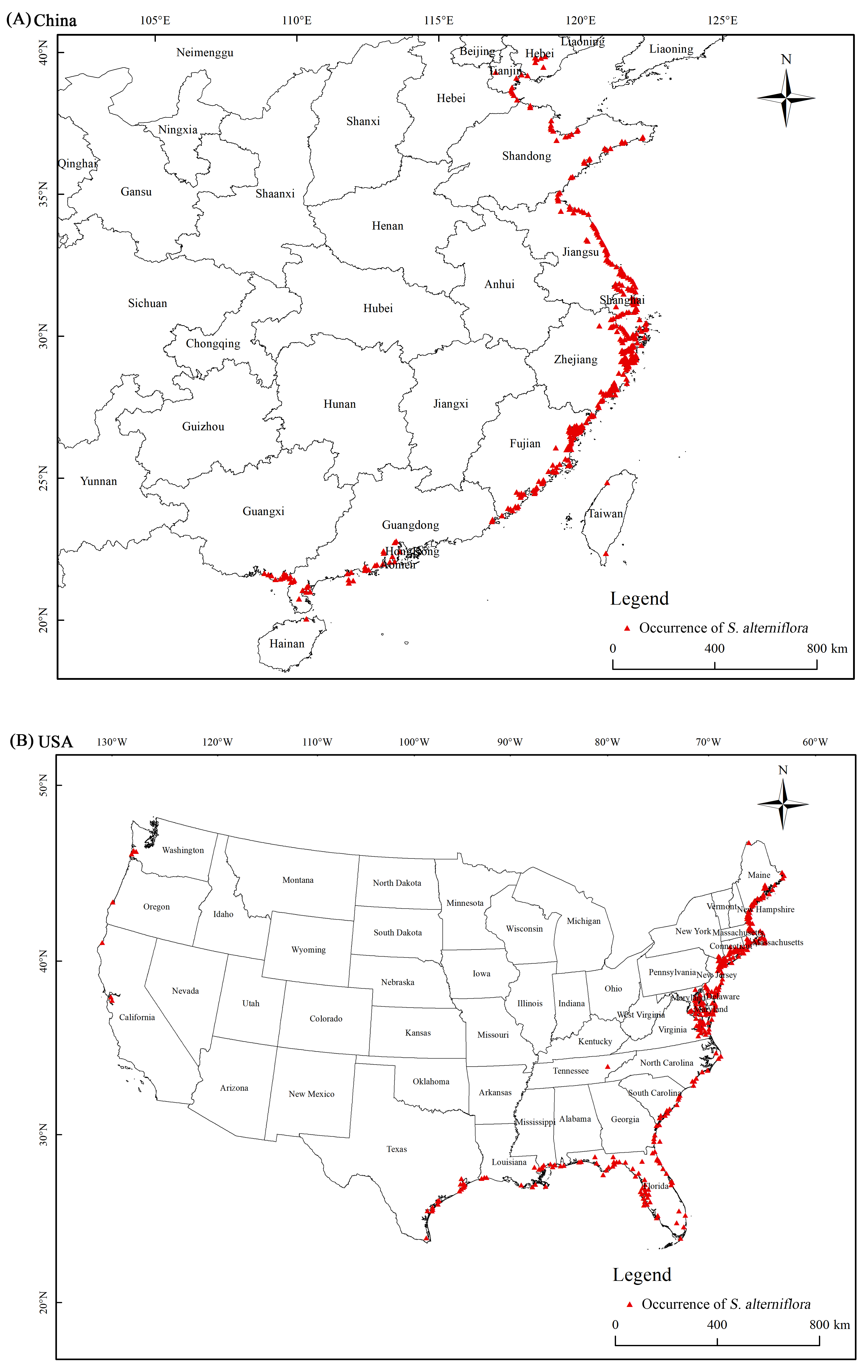
Given that S. alterniflora is largely restricted to coastal intertidal habitats, we further used the Wallace package to build a buffer zone around each effective points with strategy of “bounding box” to constrain the modeling dataset to a coastal buffer representing the species’ accessible area (M) in each region for ecological niche analysis [23], thereby excluding inland records likely attributable to georeferencing errors, cultivation, or non-establishing observations. Occurrence preprocessing and preparation for subsequent niche-comparison analyses were supported by ENMTools1.3 [24]. After all filtering steps, the final datasets comprised 358 occurrences for China and 291 occurrences for the United States for downstream SDM construction and native–invaded niche comparisons (Figure 1).

2.2. Environmental Variable Acquisition and Selection

Environmental predictors were assembled to characterize climatic constraints, coastal topography, anthropogenic pressure, land use context, and edaphic conditions relevant to S. alterniflora establishment and spread. We first obtained the 19 bioclimatic variables (BIO1–BIO19) from the WorldClim database, which summarizes annual trends, seasonality, and extreme or limiting climatic factors commonly used in SDM applications [25]. Topographic predictors were derived from a digital elevation model (DEM), including elevation and terrain derivatives (slope and aspect) computed in GIS from the DEM surface [26]. To capture human disturbance and propagule-pressure-related processes, we incorporated the Human Footprint (HFT) and Human Influence Index (HII) as broad-scale indicators of cumulative anthropogenic pressure [27]. These variables are ecologically relevant because the introduction and spread of S. alterniflora in China have been closely associated with human-mediated activities such as coastal reclamation, aquaculture development, shoreline engineering, transportation, and repeated disturbance of tidal flats. Although the occurrence records were compiled from field surveys conducted during 2023–2025, published literature, and biodiversity databases, the anthropogenic-pressure layers were used as spatial approximations of relatively persistent human influence rather than exact year-matched covariates [28]. Land use variables were included using a global landcover product (reclassified as needed for modeling) to reflect broad habitat structure and coastal land conversion [29]. Edaphic predictors were obtained from SoilGrids (e.g., sand, silt, clay fractions, and bulk density), representing soil texture and compaction conditions potentially affecting rooting and seedling performance [30]. All environmental layers were harmonized to a common geographic reference system (WGS84), clipped to the study extent (including the coastal-accessible-area mask/buffer), and resampled to a consistent spatial resolution prior to analysis (

Table 1. Environmental variables (downloaded in WorldClim; USGS EarthExplorer; NASA earth data; ESA WorldCover and ISRIC SoilGrids, etc.).

Category	Description	Abbreviation	Unit
Bioclimatic	Annual Mean Temperature	BIO1	°C
	Mean Diurnal Range	BIO2	°C
	Isothermality	BIO3	/
	Temperature Seasonality	BIO4	/
	Max Temperature of Warmest Month	BIO5	°C
	Min Temperature of Coldest Month	BIO6	°C
	Temperature Annual Range	BIO7	°C
	Mean Temperature of Wettest Quarter	BIO8	°C
	Mean Temperature of Driest Quarter	BIO9	°C
	Mean Temperature of Warmest Quarter	BIO10	°C
	Mean Temperature of Coldest Quarter	BIO11	°C
	Annual Precipitation	BIO12	mm
	Precipitation of Wettest Month	BIO13	mm
	Precipitation of Driest Month	BIO14	mm
	Precipitation Seasonality	BIO15	/
	Precipitation of Wettest Quarter	BIO16	mm
	Precipitation of Driest Quarter	BIO17	mm
	Precipitation of Warmest Quarter	BIO18	mm
	Precipitation of Coldest Quarter	BIO19	mm
Topographic	Elevation	Elev	m
	Slope	Slope	degrees
	Aspect	Aspect	degrees
Anthropogenic	Human Footprint	HFT	/
	Human Influence Index	HII	/
Land use	Land use	LULC	categorical
Soil	Sand content	Sand	%
	Clay content	Clay	%
	Silt content	Silt	%
	Bulk density	BD	kg·dm3

Note: Bioclimatic variables were included to characterize thermal and moisture constraints relevant to the growth, establishment, and potential spread of S. alterniflora. Topographic variables were used to represent low-lying coastal and estuarine settings, whereas anthropogenic variables were incorporated to capture human disturbance and propagule pressure related processes. Land-use variables reflected broad habitat structure and coastal land conversion, and soil variables were used to describe substrate conditions potentially influencing rooting and seedling establishment.

).

Because multicollinearity among predictors can inflate uncertainty and obscure interpretation in SDMs, we applied a two-step variable screening strategy combining pairwise Pearson correlation and variance inflation factor (VIF) analyses [31]. Following common practice in ecological modeling, we first calculated the Pearson correlation coefficient across candidate variables and removed one predictor from each highly correlated pair (|r| ≥ 0.7), prioritizing variables with clearer ecological relevance or broader interpretability for coastal plant invasions [32]. We then quantified residual multicollinearity using VIF and iteratively excluded variables with high inflation (VIF > 10) until all retained predictors fell below the threshold. This combined approach reduces redundancy while retaining complementary climatic, topographic, anthropogenic, land use, and soil information for subsequent SDM calibration and projection.

2.3. Environmental Space Niche Comparison Between the China and the USA

To quantify niche differences in S. alterniflora between the invaded range (China) and the native range (USA), we conducted an environmental-space niche analysis in R4.4.2 using the ecospat framework [33]. Following the PCA-env approach, niche characterization was based on the same set of predictors for both regions, including bioclimatic variables, topographic factors, anthropogenic pressure indices, and soil properties. To ensure comparability and reduce redundancy, only the final set of selected predictors was used in the niche analysis. Environmental layers were standardized and summarized across the accessible area (M) in each region, which is consistent with the view that realistic niche comparisons should be constrained to areas that have been reachable by the species over relevant timescales.

Environmental space was defined by a principal component analysis (PCA) calibrated on background environmental conditions pooled from both regions (China and USA). Niche occupancy in environmental space was estimated using kernel-smoothed occurrence densities on a grid PCA space, which explicitly accounts for environmental availability when comparing ranges. Niche overlap between China and the USA was quantified using Schoener’s D metric (0 = no overlap; 1 = complete overlap) [34]. To statistically evaluate whether niches were indistinguishable or more similar than expected by chance, we implemented ecospat’s niche equivalency and niche similarity randomization tests comparing the observed overlap against null distributions generated by repeated reshuffling procedures. In addition, niche dynamics were summarized as the proportions of stability, expansion, and unfilling to describe how the realized niche in China relates to that in the USA within the shared environmental space [35].

Although PCA-env niche comparison provides a useful framework for quantifying niche overlap, expansion, stability, and unfilling between the native and invaded ranges, it should be interpreted with caution for invasive species. This is because realized niches in introduced ranges may be affected not only by environmental filtering and dispersal limitation but also by residence time, biotic interactions, propagule pressure, and potential rapid adaptation or niche evolution after introduction. Therefore, the niche-comparison results in this study were interpreted as patterns of realized environmental niche dynamics rather than direct evidence of fixed physiological niche limits.

2.4. Species Distribution Model Construction and Evaluation

We developed ensemble species distribution models (SDMs) in R using the dismo and biomod2 packages. Twelve candidate algorithms were implemented, namely, an artificial neural network (ANN), classification tree analysis (CTA), flexible discriminant analysis (FDA), generalized additive model (GAM), generalized boosted model (GBM), generalized linear model (GLM), maximum entropy model (MaxEnt), maximum entropy model fitted using the maxnet package (Maxnet), multivariate adaptive regression splines (MARS), surface range envelope (SRE), random forest (RF), and extreme gradient boosting (XGBoost) [36]. An ensemble strategy was adopted to reduce dependence on any single algorithm and to improve the robustness and generalizability of suitability projections by integrating predictions from multiple models according to their predictive performance.

Rarefied occurrence records and the selected environmental predictors were used as model inputs. Because true absence data were unavailable, presence–pseudoabsence modeling was adopted, and 5000 pseudo-absence points were generated using the (surface range envelope, SRE) strategy implemented in biomod2. In this strategy, the environmental envelope of the presence records is first defined based on the range of selected environmental variables, and pseudo-absence points are preferentially sampled outside this envelope or in environmentally less suitable conditions. This approach reduces the probability of selecting pseudo-absences from environments that are highly similar to known presences, which is particularly relevant for invasive species whose current distribution may not yet fully occupy all suitable habitats. The number of pseudo-absence points was set to 5000 to provide sufficient background environmental information while maintaining computational efficiency and comparability among modelling algorithms. Model parameterization was implemented using the bm_ModelingOptions function in biomod2 with strategy = “bigboss” [37]. This option applies the biomod2 team’s predefined parameter settings for each candidate algorithm, rather than using algorithm defaults directly. No additional manual tuning was performed in this study. The same modelling settings were applied to the China and USA datasets to ensure comparability between the invaded and native ranges.

Model calibration and validation were repeated 10 times using a spatial block cross-validation procedure. In each replicate, occurrence records were partitioned into spatially structured training (75%) and testing (25%) subsets using 50 km spatial blocks. This block size was used to reduce spatial dependence between calibration and evaluation data while retaining sufficient occurrence records in each subset following the occurrence filtering and 5 km spatial thinning described in Section 2.1. Predictive performance was assessed on withheld evaluation data using three complementary metrics: the area under the receiver operating characteristic curve (AUC), the true skill statistic (TSS), and Cohen’s Kappa [38,39]. Because TSS is widely used in SDM evaluation and is less sensitive to prevalence effects than Kappa, single-model runs were ranked according to TSS, and only models with TSS > 0.90 were retained for ensemble construction, subsequent suitability mapping, and range-change analyses [40]. The final ensemble model was generated using TSS-based weighting, so that better-performing models contributed more strongly to the ensemble prediction.

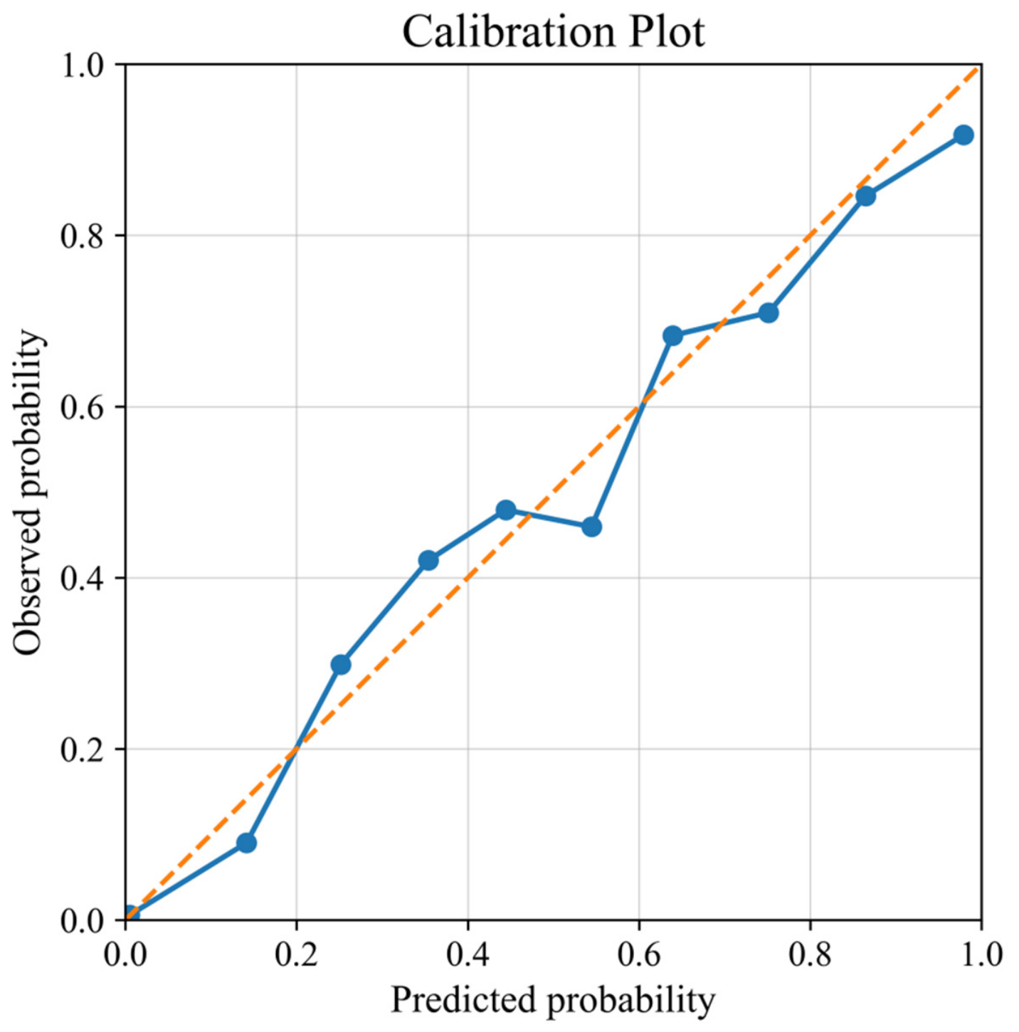
To further evaluate whether the predicted probabilities were consistent with the observed occurrence frequencies, we constructed a calibration plot comparing observed and predicted probabilities. Because discrimination metrics such as AUC and TSS mainly assess the ability of a model to distinguish presences from pseudo-absences, they do not directly evaluate probability calibration. Therefore, predicted suitability values were extracted for occurrence records and background/pseudo-absence points from the continuous prediction raster. The extracted values were grouped into 10 equal-width probability bins. For each bin, the mean predicted probability was calculated and compared with the observed probability, defined as the proportion of presence records in that bin. A 1:1 reference line was added to indicate perfect calibration. Calibration performance was further summarized using the Brier score and expected calibration error (ECE). The Brier score measures the mean squared difference between predicted probabilities and observed binary outcomes, with lower values indicating better probabilistic accuracy and calibration. ECE measures the average discrepancy between predicted probabilities and observed frequencies across probability bins, with lower values indicating better agreement between predicted suitability and observed occurrence frequency [41].

2.5. The Suitable Area Classification and Variation Under Climate Change

For the purpose of visualizing spatial patterns in habitat suitability and enabling comparison with previous studies, the continuous suitability probabilities were reclassified into four categories: 0–0.2 (non-suitable), 0.2–0.4 (low suitability), 0.4–0.6 (moderate suitability), and 0.6–1.0 (high suitability) [42]. These categories were intended only to depict relative gradients in model predicted habitat suitability and should not be interpreted as absolute ecological thresholds of S. alterniflora occurrence, persistence, or ecological performance. Therefore, the continuous probability output was treated as the primary basis for model interpretation, whereas the categorized suitability classes were used principally for map display and comparison with earlier studies.

To quantify suitable-area changes under future climate scenarios, both the present and future suitability rasters were first converted to binary maps by ArcGIS Reclassify, using a TSS-optimized cutoff value as a threshold of suitable (1) and non-suitable (0). Change categories were then derived with Raster Calculator (map algebra) by overlaying present and future binary rasters. Specifically, the raster difference among future and present identified expansion area as +1 (0 → 1) and contraction area as −1 (1 → 0). Pixels with a difference of 0 were subsequently separated into stable area (1 → 1) and persistent non-suitable area (0 → 0) by overlaying or combining the two binary layers where 2 indicates 1 → 1 and 0 indicates 0 → 0. Therefore, the final change classes comprised expansion area (0 → 1), stable area (1 → 1), contraction area (1 → 0), and non-suitable area (0 → 0), enabling pixel-based mapping and area accounting of range dynamics under climate change [43].

2.6. Multivariate Environmental Similarity Surface Analysis

To assess whether the estimated niche unfilling was influenced by environmental non-analogy between the native and invaded ranges, we conducted a multivariate environmental similarity surface (MESS) analysis using the same final set of environmental variables retained for the PCA-env niche comparison. Environmental conditions in the USA were used as the reference environmental space, and environmental conditions in China were projected against this reference to identify regions with analogous and non-analogous environments. The resulting MESS covered the broader environmental background of the invaded range in China, including the area involved in the bounding-box-based PCA-env niche analysis. Positive MESS values indicated analogous environments, where Chinese environmental conditions fell within the range of environmental conditions available in the native range, whereas negative MESS values denoted non-analogous environments, where at least one predictor exceeded the environmental envelope of the native range. This analysis allowed us to identify whether the environmental space associated with the inferred niche-unfilling pattern occurred under comparable or non-comparable environmental conditions between the two ranges.

2.7. Uncertainty

To improve the transparency of uncertainty reporting and further evaluate the robustness of our predictions, we conducted an auxiliary algorithm-related uncertainty analysis by comparing the final ensemble model (EM) with the high-performing single model algorithms retained after model screening (TSS > 0.90), namely, the generalized additive model (GAM), generalized boosting model (GBM), and random forest (RF) in the invaded range. First, the continuous habitat suitability rasters generated by the EM, GAM, GBM, and RF were converted into binary suitable/unsuitable maps using the same thresholding rule applied in the suitable area change analysis. Pairwise spatial overlay analyses were then performed between the EM and each of the three single model predictions (EM vs. GAM, EM vs. GBM, and EM vs. RF). Based on the overlay results, pixels were classified into three categories: (i) unsuitable area, (ii) uncertainty area, and (iii) agreement area. The unsuitable area referred to regions predicted as unsuitable by both models, the uncertainty area referred to regions where the two models differed in suitability prediction, and the agreement area referred to regions predicted as suitable by both models. Within this framework, the uncertainty area was interpreted as the spatial expression of algorithm-related predictive uncertainty, whereas the agreement area was understood to indicate areas where the final ensemble projection was relatively robust and showed high spatial consistency [43].

3. Results

3.1. Niche Analysis Between Native and Invaded Range

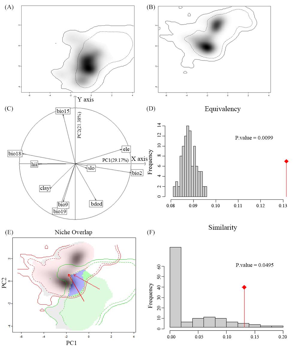
The native and invaded niche shape of S. alterniflora are shown in Figure 2a,b, which clearly show the specific niche characteristics at two places. Principal component analysis (PCA) of the environmental conditions—PC1 (29.17%) and PC2 (21.38%)—can comprehensively explain 50.55% of total environment space. PC1 was positively driven by mean diurnal temperature range (bio2); PC2 was also positively influenced by precipitation seasonality (bio15). It is clear that the ecological niche of invasive S. alterniflora is vulnerable to variations in temperature and precipitation. The niche overlap value of S. alterniflora between the native and invaded range (Schoener’s D) is 0.13. This indicates that the environment space and niche are shifting toward the places with lower temperature and higher precipitation. The equivalency (d) and similarity test (f) obviously support the null hypothesis (p < 0.05), and the niche observed (the red line with a diamond on the right) reveals the differences between the two tests. The observed niche falls outside the 95% confidence interval in the equivalency test; by contrast, the observed niche falls within the 95% confidence interval in the similarity test. Therefore, we can conclude that the environment niches of S. alterniflora, with respect to the native and invaded ranges, are similar but not equal. The unfilling value of S. alterniflora is 0.36, which means that in the invaded range (China), there are many spaces with similar environment conditions that S. alterniflora could occupy in the future.

3.2. Model Evaluation Performance with Ensemble Model

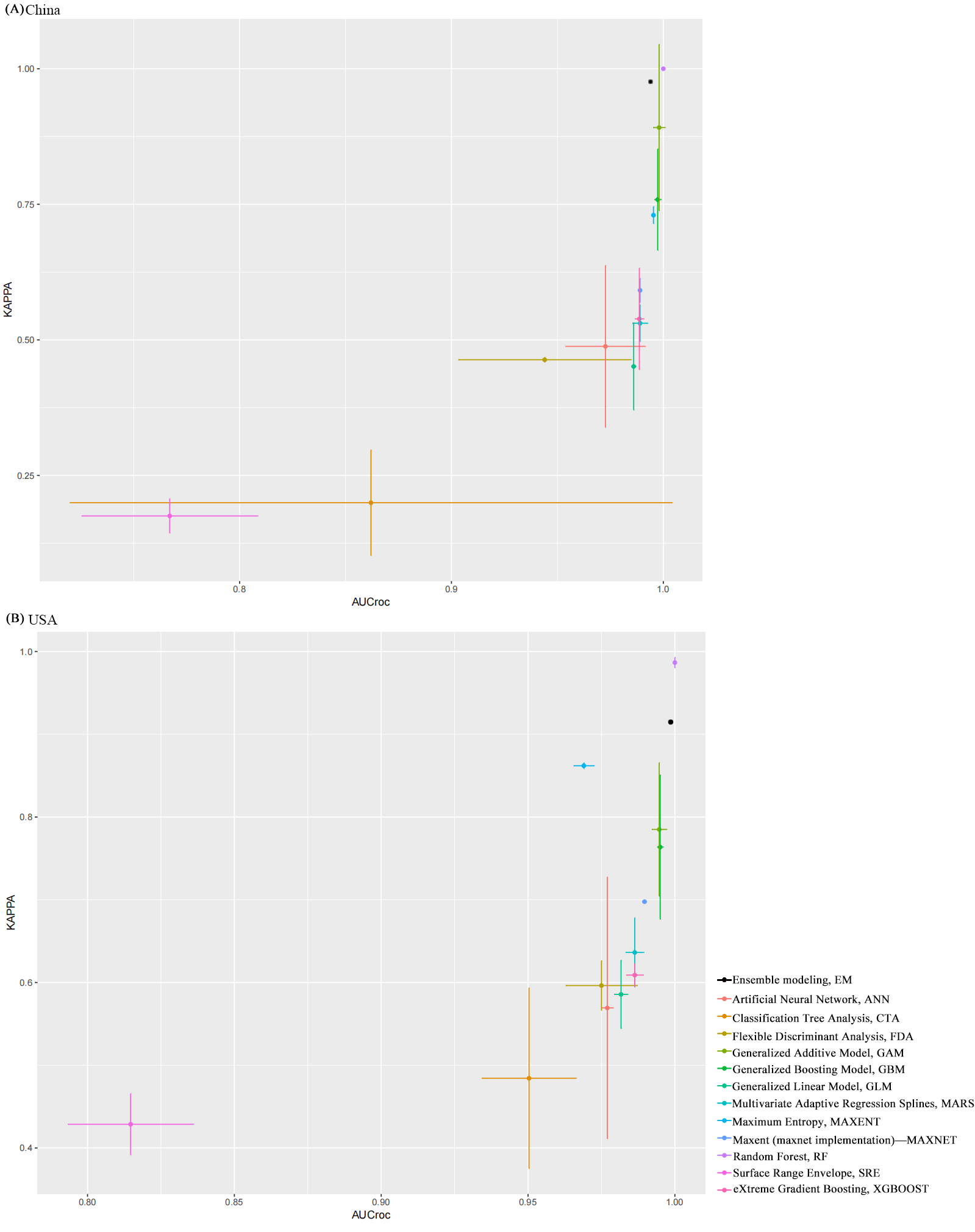
Across both China and the USA, several algorithms have demonstrated strong predictive skill. To ensure consistency between the native and invaded range, only model runs with TSS > 0.90 were retained for subsequent modeling, and all retained runs were integrated using TSS-based weights. This preserved information from multiple high-performing algorithms and ensured that China and the USA were analyzed under the same ensemble framework. The final ensemble model also performed well, with evaluation scores of TSS = 0.994, Kappa = 0.925, and AUC = 0.980 for China, and TSS = 0.935, Kappa = 0.915, and AUC = 0.993 for the USA (Figure 3). Overall, this strategy reduced dependence on any single algorithm and improved the comparability of native and invaded range predictions.

The calibration plot showed a clear positive relationship between predicted probability and observed probability (Figure 4). Across the 10 probability bins, the observed proportion of presences generally increased with mean predicted probability, indicating that higher predicted values corresponded to higher observed occurrence frequencies. The calibration curve was broadly close to the 1:1 reference line, with only moderate deviations in several intermediate probability bins. The Brier score was 0.023, and the expected calibration error was 0.0066, suggesting a low overall calibration error. These results indicate that the high AUC and TSS values were not interpreted solely as discrimination metrics but were further supported by the observed predicted probability relationship. Therefore, the model output provides a reliable relative suitability estimation.

3.3. Analysis of the Dominated Environment Variables

The variable importance analysis, which quantifies the relative contribution of each predictor to the final ensemble model, revealed a pronounced dominance of a single topographic factor in determining the potential distribution of the studied species.

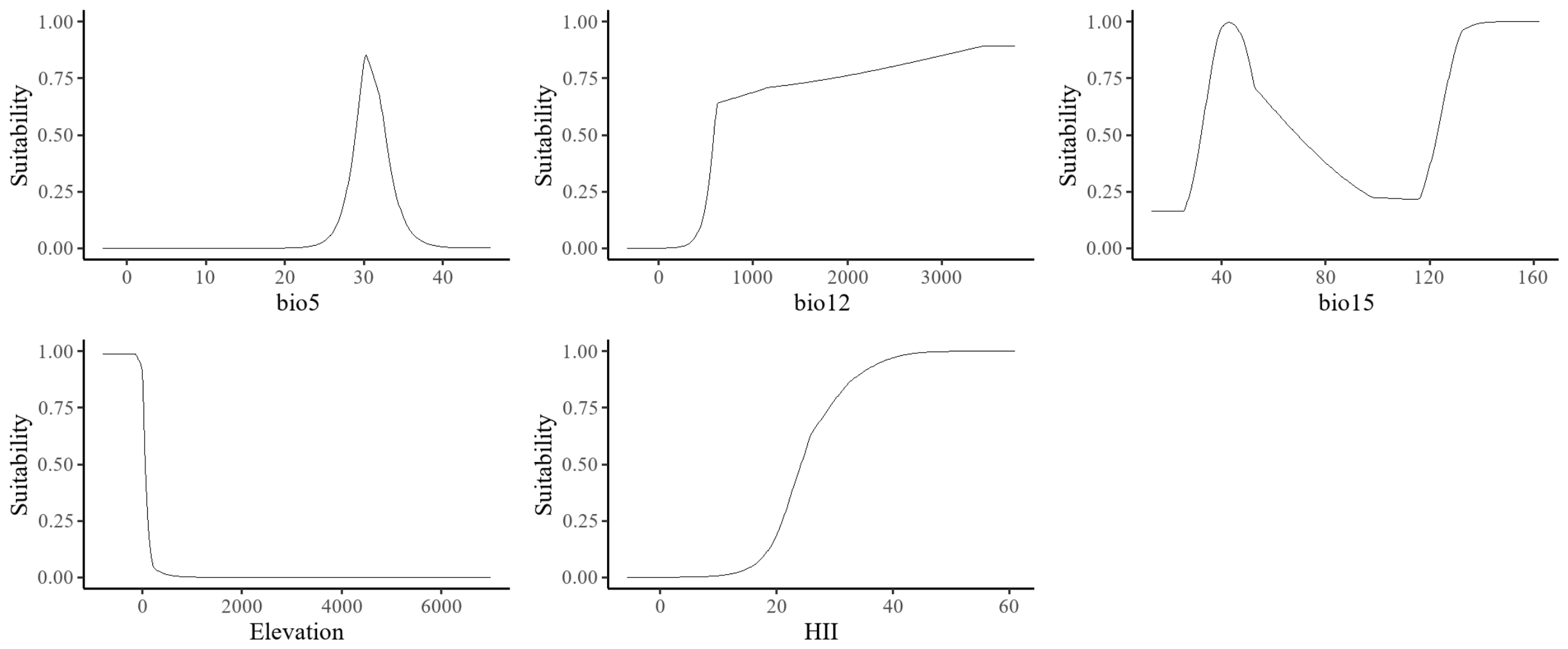
The single factor response curves (Figure 5) indicated that elevation was the strongest predictor of the potential distribution of S. alterniflora. Predicted suitability was the highest in low-elevation areas (below 100 m) and declined rapidly with increasing elevation. This pattern indicates that elevation mainly captured the species’ broad confinement to low-lying coastal and estuarine environments, rather than a fine-scale tidal-height threshold. bio5 showed the highest suitability at approximately 28–33 °C, with a peak near 30 °C. Suitability for bio12 increased markedly above 600 mm annual precipitation and remained relatively high between 600 and 3500 mm. bio15 displayed a bimodal response, with higher suitability mainly within 38–75 and 125–160. The response curve for HII further suggested relatively high suitability in areas with moderate-to-high human influence, especially when HII values exceeded 25.

At the national scale across China, variable percent contribution (

Table 2. Importance of environment variables in China.

Variable	Contribution Rate
Elevation	73.6
Human influence index (HII)	6
Annual precipitation (bio12)	5.2
Max temperature of warmest month (bio5)	4.9
Precipitation seasonality (bio15)	4.3
Slope	3
Land use	1.5
Aspect	0.8
Mean temperature of wettest quarter (bio8)	0.4
Clay	0.2
Isothermality (bio3)	0

) indicates that elevation is the dominant predictor (73.6%), suggesting that the modeled suitable habitat for S. alterniflora is primarily associated with low-lying coastal environments. The next most influential variables were the Human Influence Index (HII, 6.0%), annual precipitation (bio12, 5.2%), maximum temperature of the warmest month (bio5, 4.9%), and precipitation seasonality (bio15, 4.3%), implying that anthropogenic pressure and regional hydrothermal conditions provide additional explanatory power. In contrast, slope contributed relatively little (3.0%), and land use (1.5%), aspect (0.8%), and the remaining soil/climatic variables contributed only marginally (≤0.4%). To evaluate whether the dominant contribution of elevation masked the effects of other predictors, we conducted an additional sensitivity analysis by refitting the China model after excluding elevation. The no-elevation ensemble model still showed acceptable predictive performance (AUC = 0.975, TSS = 0.990, Kappa = 0.930), and the predicted suitable habitats remained mainly concentrated along the coastal belt. After elevation was removed, the relative importance of anthropogenic and hydroclimatic variables increased, with HII (46.5%), BIO12 (31.5%), BIO5 (16.5%), and BIO15 (3.2%) becoming the main predictors, whereas the remaining variables contributed only marginally. These results suggest that although elevation captured the broad coastal and low-lying distributional constraint of S. alterniflora, the overall coastal suitability pattern was also supported by anthropogenic disturbance and regional hydroclimatic conditions.

3.4. The Potential Suitable Range in China at Present

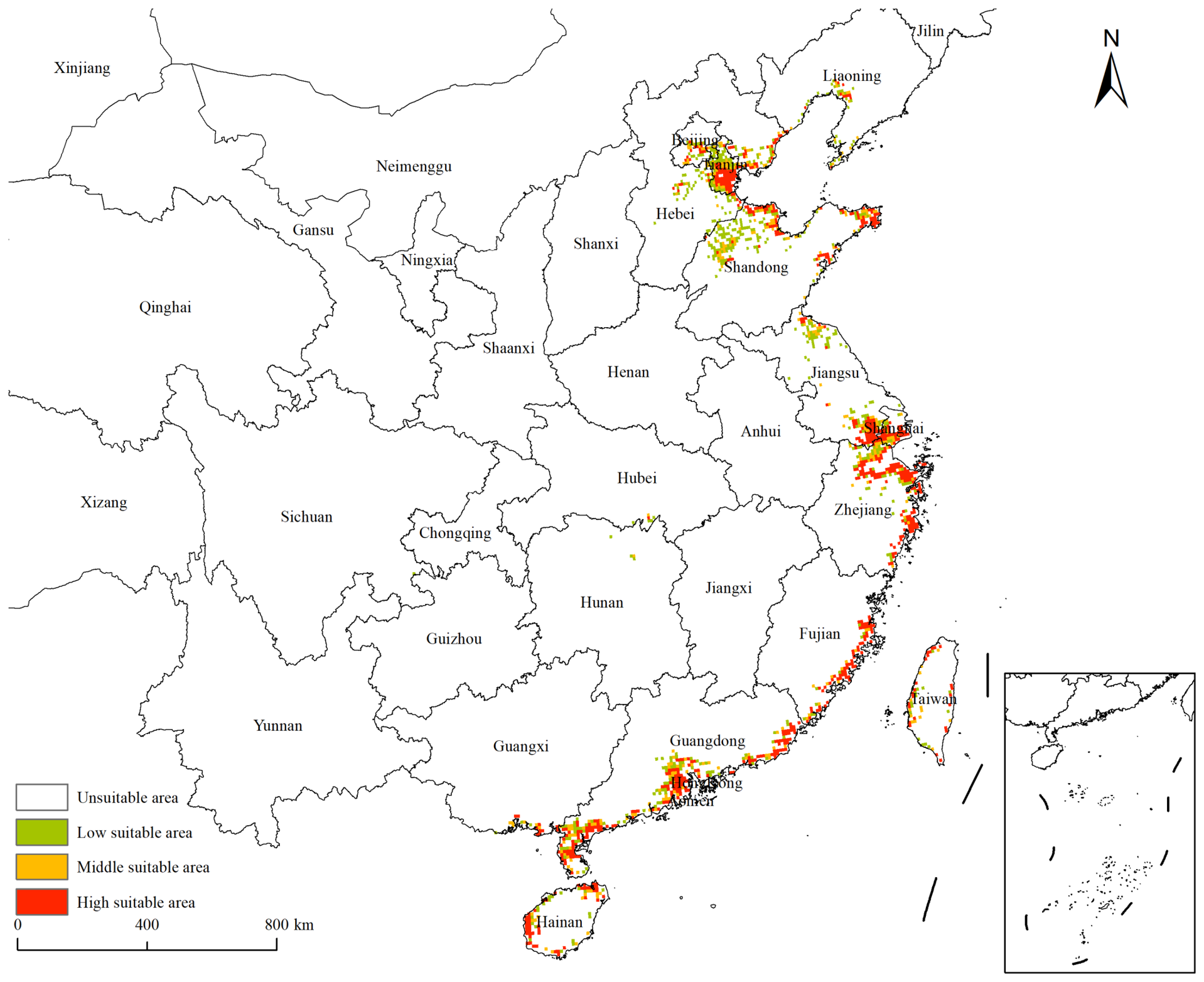
As shown in Figure 6, the potential suitable habitat for S. alterniflora in China exhibits a pronounced coastal belt-like pattern. High suitability is largely confined to the Bohai Rim and the coastal zones of the Yellow Sea, East China Sea, and South China Sea, forming continuous to semi-continuous strips along the shoreline, with clear spatial clustering in major estuarine and bay wetland complexes. In contrast, most inland areas are classified as unsuitable, indicating that the species’ potential distribution at the national scale is strongly constrained by coastal wetland habitat conditions.

In terms of suitability classes, the low-suitability area covers 3.78 × 10⁴ km², the middle-suitability area covers 2.3 × 10⁴ km², and the high-suitability area covers 5.25 × 10⁴ km², yielding a total potential suitable area of 11.42 × 10⁴ km². These correspond to 33.10%, 20.93%, and 45.97% of the total suitable area, respectively. Spatially, low- and medium-suitability zones generally form relatively continuous marginal and transitional belts along the coast, linking discrete high-suitability patches. High-suitability zones are more spatially concentrated yet account for the largest share of the suitable area, and they are primarily associated with key estuaries, embayments, and well-developed intertidal wetland segments, representing core areas where establishment and further expansion are most likely and should be prioritized for management attention. Although the predicted suitable habitats were mainly concentrated along the coastline, a small number of suitable patches also appeared in areas relatively far from the coast in the current suitability map. These inland or weakly coast-connected patches should not be directly interpreted as confirmed suitable habitats for natural establishment of S. alterniflora. Instead, they may reflect environmental similarity in the predictor space and should be regarded as areas with higher interpretative uncertainty that require further field verification.

3.5. The Variation in Potential Distribution Area in China Under Climate Change

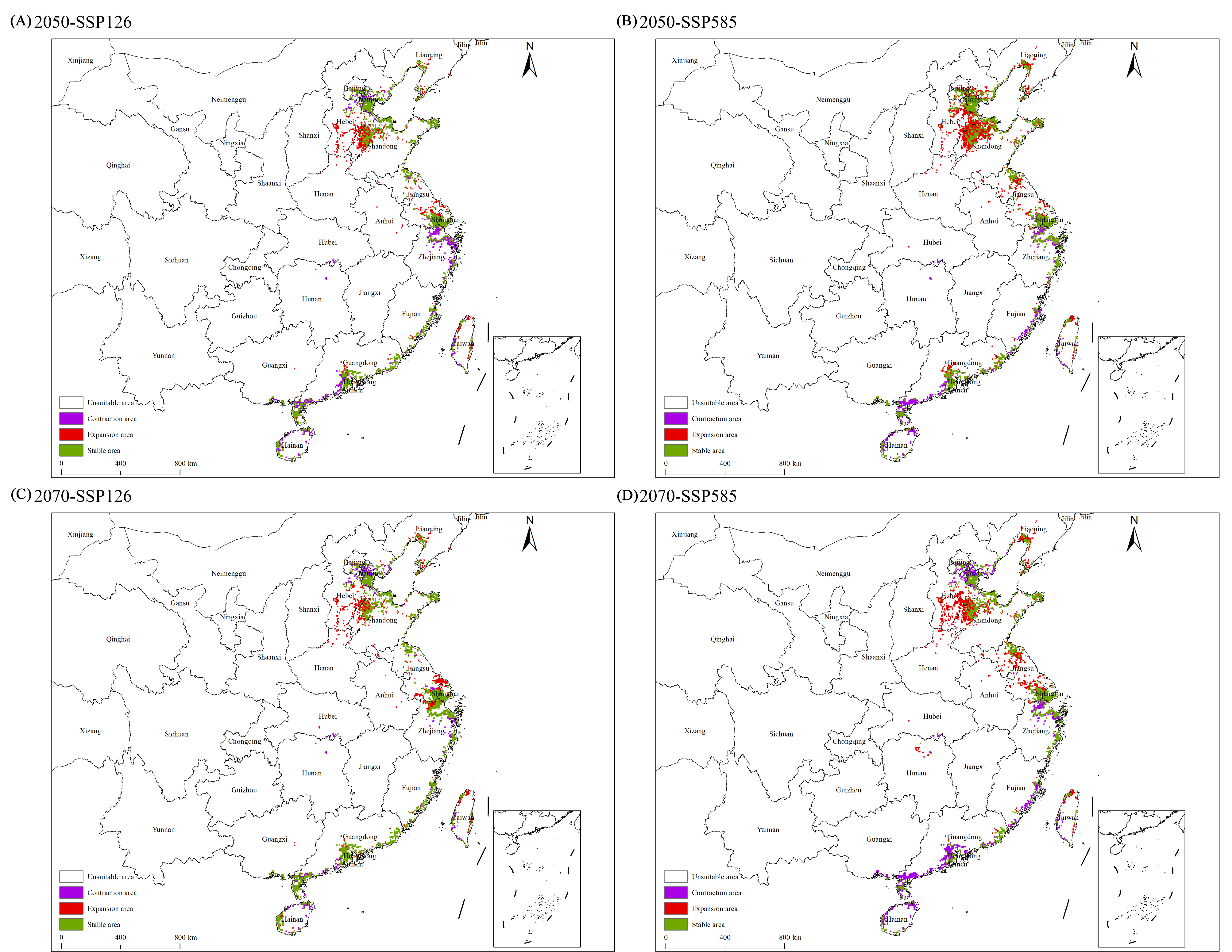
As shown in Figure 7, projected changes in suitable habitat for S. alterniflora under the four future scenarios display a clear coastal-belt response, with changes concentrated in key coastal wetland regions, including the Bohai Rim, the Yangtze River Delta, and the southeastern to southern China coastline. Across scenarios, stable suitable habitat dominates, indicating a high degree of persistence of suitability within the present-day coastal distribution belt. However, the relative magnitudes of habitat gain and loss differ markedly between emissions pathways. Compared with SSP126, SSP585 generally produces larger increases in suitable habitat, with more extensive additions along the northern coast and around the Yangtze River Delta. By 2070, adjustments remain largely confined to the existing coastal suitability belt, with gains and losses occurring in different coastal segments simultaneously. This pattern suggests scenario-dependent regional reorganization of the potential distribution boundary, while overall suitability remains strongly constrained by coastal wetland conditions.

Area estimates further quantify these patterns (

Table 3. Different ranks of suitable area change under climate change (×10⁴ km²).

Suitable Rank	2050-SSP126	2050-SSP585	2070-SSP126	2070-SSP585
Stable area	8.69	9.45	9.82	7.46
Expansion area	3.24	5.71	3.55	5.18
Contraction area	3.26	2.5	2.13	4.5

). Stable habitat area under 2050-SSP126, 2050-SSP585, 2070-SSP126, and 2070-SSP585 is 8.69 × 10⁴ km², 9.45 × 10⁴ km², 9.82 × 10⁴ km², and 7.46 × 10⁴ km², respectively. Stable habitat is lowest under 2070-SSP585 relative to the other three future scenarios, although it still accounts for a substantial proportion of the current suitable area. Habitat gains are larger under SSP585 (5.71 × 10⁴ km² in 2050-SSP585 and 5.18 × 10⁴ km² in 2070-SSP585) than under SSP126 (3.24 × 10⁴ km² in 2050-SSP126 and 3.55 × 10⁴ km² in 2070-SSP126), implying stronger expansion potential under the higher-emissions pathway. Habitat losses also vary substantially. Specifically, losses are 3.26 × 10⁴ km² in 2050-SSP126 versus 2.50 × 10⁴ km² in 2050-SSP585, while by 2070, they decrease to 2.13 × 10⁴ km² under SSP126 but increase to 4.50 × 10⁴ km² under SSP585, the highest among all scenarios. Taken together, SSP585 is characterized by larger potential gains but, in the late-century projection, also a pronounced increase in losses, indicating concurrent expansion and contraction dynamics along the coast.

3.6. MESS-Based Assessment of Environmental Analogy

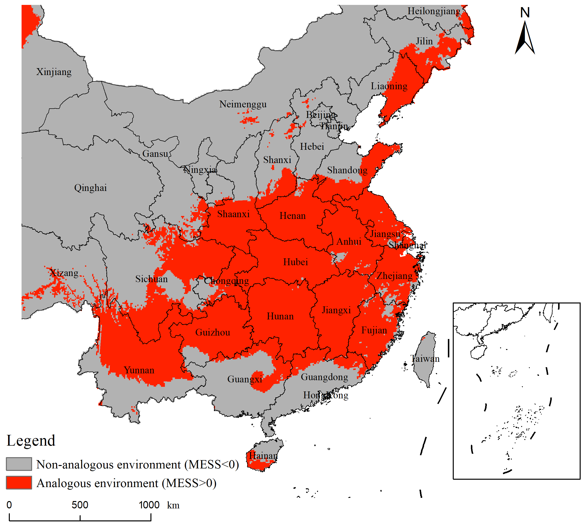
The MESS analysis showed clear spatial heterogeneity in environmental analogy between China and the USA based on the selected predictor variables used in this study (Figure 8). Across the analyzed environmental background in China, areas with positive MESS values accounted for 46.22%, indicating that these areas fell within the environmental envelope of the USA native range with respect to the predictors used in this study. In contrast, 53.78% of the analyzed area showed negative MESS values, representing non-analogous environments in which at least one predictor exceeded the environmental range available in the native range.

To further evaluate the environmental credibility of the predicted distribution, we overlaid the current binary suitability map with the MESS classification. The overlay analysis showed that 37.81% of the current predicted suitable habitat occurred within analogous environments, whereas 62.19% occurred under non-analogous conditions. This indicates that part of the predicted suitable habitat is located under environmental conditions comparable to those available in the native range, whereas a larger proportion involves environmental extrapolation and should therefore be interpreted cautiously.

It should be noted that the MESS analysis evaluates environmental analogy only with respect to the selected predictor set, rather than directly assessing the ecological suitability of S. alterniflora. Because variables explicitly representing tidal regime, seawater salinity, salt-spray exposure, and coastal hydrological connectivity were not included, analogous environments located far inland should not be interpreted as biologically equivalent habitats or confirmed areas for natural establishment of S. alterniflora. Instead, these areas may reflect similarity in broad-scale climatic, topographic, soil, land-use, or anthropogenic conditions.

3.7. Algorithm-Related Spatial Uncertainty Analysis

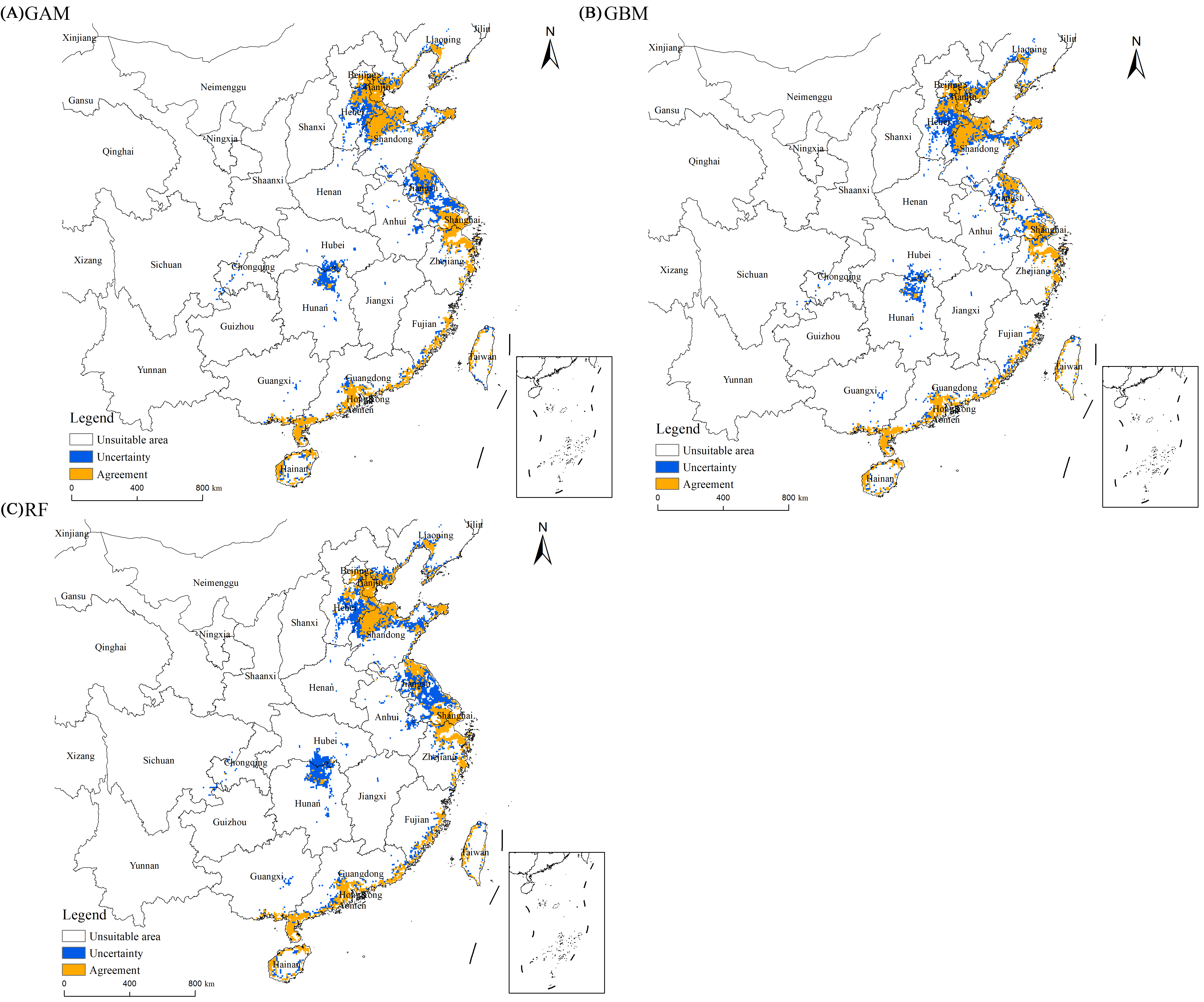
The spatial overlay comparisons between the ensemble model (EM) and the three high-performing single models (GAM, GBM, and RF) revealed pronounced spatial heterogeneity in prediction agreement and disagreement along the coast of China (Figure 9). Overall, areas of agreement in suitable habitat were distributed continuously or semi-continuously along the eastern and southeastern coastal belt of China, with major concentrations in the Bohai Rim, the Shandong Peninsula and adjacent coastal areas, the Yangtze River Delta, and the southeastern to southern coastline. These regions, therefore, exhibited relatively high spatial consistency among algorithms and can be regarded as the core areas where predictions of potential suitable habitat are comparatively robust. In contrast, uncertainty areas were mainly located in the marginal transition zones surrounding these core suitable belts, as well as in some scattered inland patches, indicating that habitat suitability in these areas was more sensitive to algorithm choice and thus subject to higher spatial predictive uncertainty.

Area statistics further quantified the degree of agreement and uncertainty among algorithms. In the comparison between the GAM and EM, the uncertainty area was 11.88 × 10⁴ km², whereas the agreement in suitable area reached 17.77 × 10⁴ km². For the GBM versus the EM, the uncertainty area was 11.87 × 10⁴ km², and the agreement in suitable area was 17.21 × 10⁴ km². For RF versus the EM, the uncertainty area increased to 15.25 × 10⁴ km², while the agreement in suitable area was 17.57 × 10⁴ km². Overall, the extent of agreement in suitable area between the single models and the EM was broadly similar, ranging from 17.21 to 17.77 × 10⁴ km², suggesting that the major suitable coastal belt was identified consistently across algorithms and therefore exhibited relatively high spatial robustness. However, the extent of uncertainty varied among models, with RF showing the largest uncertainty area relative to the EM, clearly exceeding those of the GAM and GBM. This result indicates that RF diverged more strongly from the EM in spatial prediction and contributed a comparatively higher level of algorithm-related uncertainty.

4. Discussion

This study provides a spatial assessment of the invasion risk of S. alterniflora in China by integrating native–invaded niche comparisons with ensemble species distribution model projections under current and future climate scenarios. Three findings are particularly important. First, niche overlap between the native and invaded range was low, whereas niche unfilling in the invaded range in China remained substantial, indicating that environmentally suitable space in the invaded range has not yet been fully occupied. This result is consistent with previous studies showing that S. alterniflora has undergone niche shifts between its native and invaded range and that suitable environmental space in the invaded range remains incompletely filled [44]. Second, projected suitable habitat in China was predominantly concentrated in coastal and estuarine regions, although a small number of inland or weakly coast-connected suitable patches were also predicted, and elevation emerged as the dominant predictor of habitat suitability [45,46]. Third, although stable suitable habitat dominated under all future scenarios, the relative balance between expansion and contraction varied among scenarios, suggesting that future changes are more likely to involve regional reorganization of suitable habitat than simple unidirectional range expansion. Previous climate-scenario studies of S. alterniflora likewise indicate pronounced spatial heterogeneity in future distributional change, potentially accompanied by poleward expansion, local contraction, and shifts in secondary invasion risk [47,48,49]. Last but not least, although the KAPPA or AUCroc values of some single candidate models are higher than those of ensemble models such as RF, etc., ensemble models can effectively reduce over-fitting, decrease variance, and largely enhance the transferability of modeling prediction [50]. Overall, these results suggest that both currently invaded coastal wetlands with persistent suitable habitat and presently unoccupied but potentially suitable areas may face substantial invasion risk in the future.

Our results are broadly consistent with those of previous studies of S. alterniflora and other invasive coastal plants in China. The dominant role of elevation is ecologically plausible because S. alterniflora is mainly distributed in low-lying coastal wetlands, estuaries, and intertidal flats, where topographic position is closely associated with tidal inundation, flooding frequency, salinity exposure, and sedimentary conditions, all of which strongly influence its growth, reproduction, and competitive performance relative to native species [50,51,52]. However, the elevation layer used in this study was derived from DEM data and was not standardized to local tidal data such as mean sea level, mean low water, or mean high water. Given the large spatial extent of the Chinese coastline and the strong regional variation in tidal range, raw DEM elevation should not be interpreted as a directly comparable measure of tidal height across all coastal regions. Therefore, the high contribution of elevation likely reflects both the broad ecological restriction of S. alterniflora to low-lying coastal environments and the model’s discrimination between coastal/intertidal and inland environments. This limitation does not weaken the national-scale coastal-belt pattern identified by the model, but it indicates that fine-scale predictions of local tidal suitability should be interpreted cautiously. Future studies should incorporate tidal-data-normalized elevation, inundation frequency, hydrodynamic conditions, and sediment properties to improve the mechanistic interpretation of elevation effects. Likewise, the concentration of suitable habitats in the Bohai Rim, the Yangtze River Delta, and the southeastern to southern coastal regions is consistent with the continued expansion of S. alterniflora along the Chinese coast and its marked aggregation in estuarine and tidal-flat systems [5,45,46,47,48]. From a biological and ecological perspective, this coastal concentration is also consistent with the species’ life-history traits. S. alterniflora can reproduce clonally through rhizomes and sexually through abundant seed production, tolerate salinity and periodic inundation, and disperse effectively through tidal currents and waterborne transport of seeds or vegetative fragments. These traits make estuaries, tidal flats, bays, and other low-lying coastal wetlands particularly favorable for establishment and expansion, especially where human disturbance creates open substrates or reduces resistance from native vegetation [53]. The relatively high contribution of anthropogenic pressure, represented here by the Human Influence Index, further indicates that the spread of S. alterniflora is constrained not only by climate and geomorphology; it is also closely associated with intense coastal human disturbance, reclamation activities, and management responses [5,48,54]. In addition, the combination of a low Schoener’s D value and relatively high niche unfilling further indicates that S. alterniflora has not yet occupied the full range of environmentally available conditions in its invaded range in China. In practical terms, this means that the current invaded distribution should not be interpreted as the full potential range of the species in China; rather, especially where dispersal pathways remain active and human disturbance continues to facilitate spread, coastal sectors that are environmentally suitable but not yet occupied may remain vulnerable to future invasion [15].

Future projections in this study indicate that suitable habitats will likely remain concentrated within the existing coastal zone, although the balance among habitat persistence, gain, and loss differs among scenarios. In all projections, stable areas accounted for a large proportion, suggesting that extensive stretches of the currently suitable coastal belt are likely to continue providing favorable conditions for invasion. Moreover, under climate change, habitat expansion and contraction co-occurred across all scenarios, with this pattern being most pronounced under SSP585. This suggests that the effect of climate change on the potential distribution of S. alterniflora is manifested primarily as a heterogeneous reorganization of suitable habitat, rather than as a unidirectional increase or decrease in invasion risk at the overall scale. This interpretation is consistent with recent studies reporting strong spatial heterogeneity in future distributional responses of S. alterniflora [16,44]. In addition, the uncertainty analysis improved the interpretability of these projections. Areas of agreement between the ensemble model and representative single-model outputs were mainly concentrated within the major coastal belt, whereas disagreement was more common in transitional margins and scattered inland patches. This suggests that core coastal wetland habitats identified as suitable by multiple algorithms can be interpreted with greater confidence, whereas marginal areas should be treated more cautiously. This approach is also consistent with recommendations from the SDM literature emphasizing the spatially explicit representation of model uncertainty and prediction stability [54,55,56].

Several limitations of this study should also be acknowledged. First, although continuous suitability was the primary model output, analyses of range change still relied on binary suitable/unsuitable maps. While this approach facilitates the identification of stable, expanding, and contracting areas, it inevitably introduces threshold dependence. The TSS-optimized threshold used in this study is methodologically reasonable, but different thresholding schemes may still affect area estimates, particularly in marginal zones near suitability boundaries. Accordingly, the values reported in Table 3 should be interpreted as scenario-dependent estimates rather than precise forecasts. Recent studies likewise show that different binarization thresholds can substantially influence estimates of current range size and the magnitude of future range shifts [57,58]. Second, although the environmental predictors were carefully screened, key coastal processes such as tidal hydrodynamics, salinity heterogeneity, coastal connectivity, and local sediment conditions were not explicitly quantified. Therefore, the few inland or weakly coast-connected suitable patches predicted by the model should be interpreted as areas with higher uncertainty rather than confirmed habitats for self-sustaining S. alterniflora populations. In addition, DEM-derived elevation was not standardized to local tidal datums, so its effect should be viewed as a broad-scale signal of coastal position and low-lying terrain rather than a directly comparable measure of tidal height across regions. Third, future projections in this study modified only the climatic variables under SSP126 and SSP585, whereas non-climatic predictors, including DEM-derived elevation, human influence, land use, and soil properties, were kept constant. This assumption should be interpreted with particular caution for a tidal-wetland species such as S. alterniflora because sea-level rise, shoreline engineering, reclamation, and land use change may substantially alter the availability and spatial position of suitable coastal wetlands. Therefore, the future projections presented here should be viewed as climate-driven habitat suitability scenarios rather than complete forecasts of future coastal wetland availability. Future studies should further incorporate sea-level rise, tidal inundation, and coastal land use change to improve the mechanistic interpretation of invasion risk projections. Fourth, the uncertainty analysis mainly focused on spatial discrepancies among modeling algorithms and did not systematically partition other potential sources of uncertainty, such as threshold selection, climate models, and dispersal assumptions. Therefore, the results of this study are better viewed as strategic indicators of invasion risk rather than deterministic forecasts of future occupancy patterns. Recent SDM studies have similarly emphasized the need to move beyond final suitability maps by more explicitly characterizing uncertainty through source decomposition, variance partitioning, and analyses of spatial consistency [54,55,56,57,58].

These results also have clear management implications. Because stable suitable habitat remained extensive across all future scenarios, currently invaded coastal areas are unlikely to become naturally unsuitable in the near term and therefore still require continued surveillance, containment, and post-removal monitoring. At the same time, the presence of expansion zones indicates that, particularly under the high-emissions scenario, additional coastal sections may become potentially suitable in the future. These newly suitable or marginally suitable areas should therefore be prioritized for early warning and preventive monitoring, especially in estuaries, deltas, embayments, and other low-elevation intertidal systems connected to existing invasion fronts [5,16]. The uncertainty analysis further suggests that management decisions should be spatially stratified: areas with high model agreement can be treated as priority management units, whereas algorithm-sensitive transitional zones should be subject to intensified field verification before major interventions are implemented. Accordingly, a more robust management strategy would be to develop a tiered control framework that integrates sustained management of invasion cores, forward-looking surveillance of potential expansion zones, and cautious evaluation of highly uncertain marginal areas. Recent national-scale assessments of control outcomes and field-based eradication studies also support a management strategy centered on sustained control, effectiveness evaluation, and prevention of reinvasion [5,59].

Overall, this study indicates that the future invasion risk of S. alterniflora in China will remain concentrated primarily in low-elevation coastal wetlands and that climate change is more likely to reorganize the spatial pattern of risk than simply to promote overall range expansion [60]. By integrating niche comparison, ensemble SDM projections, and spatial uncertainty analysis, this study provides a more management-relevant basis for identifying persistent and emerging invasion hotspots. Future research should incorporate more direct coastal-process variables, test the sensitivity of range-change estimates to alternative thresholding schemes, and link suitability projections with dispersal pathways and management history in order to improve the explanatory power and practical value of invasion risk forecasting [16,54,55].

5. Conclusions

By integrating occurrence records from the invaded range (China) and the native range (USA) and harmonizing multi-source predictors, we built biomod2 ensemble species distribution models and compared native–invaded climatic niche spaces. The ensemble model achieved high predictive performance in both regions (China: TSS = 0.994, AUC = 0.980; USA: TSS = 0.935, AUC = 0.993). Elevation was the dominant constraint on potential distribution (73.6%), and niche analyses indicated low overlap (Schoener’s D = 0.132) with substantial niche unfilling in China (0.36), suggesting that additional suitable environmental space remains available for future colonization.

Current suitable habitats are concentrated in coastal intertidal wetlands from the Bohai Rim through the Yellow Sea–East China Sea to the South China Sea coasts. Under future climate scenarios, suitability changes are largely confined to existing coastal wetland extents, with stable suitable area predominating (8.69~9.82 × 10⁴ km²) and relatively stronger expansion under SSP585. These projections provide a practical basis for risk zoning and for prioritizing surveillance and early interventions in stable and newly suitable coastal segments to support adaptive coastal wetland management.

References

1. Diagne, C.; Leroy, B.; Vaissière, A.C.; Gozlan, R.E.; Roiz, D.; Jarić, I.; Salles, J.M.; Bradshaw, C.J.A.; Courchamp, F. High and rising economic costs of biological invasions worldwide. Nature 2021, 592, 571–576. [Google Scholar] [CrossRef] [PubMed]
2. Fantle-Lepczyk, J.E.; Haubrock, P.J.; Kramer, A.M.; Cuthbert, R.N.; Turbelin, A.J.; Crystal-Ornelas, R.; Diagne, C.; Courchamp, F. Economic costs of biological invasions in the United States. Sci. Total Environ. 2022, 806, 151318. [Google Scholar] [CrossRef] [PubMed]
3. Pyšek, P.; Hulme, P.E.; Simberloff, D.; Bacher, S.; Blackburn, T.M.; Carlton, J.T.; Dawson, W.; Essl, F.; Foxcroft, L.C.; Genovesi, P.; et al. Scientists’ warning on invasive alien species. Biol. Rev. 2020, 95, 1511–1534. [Google Scholar] [CrossRef]
4. Zhang, X.; Zhao, J.; Wang, M.; Li, Z.; Lin, S.; Chen, H. Potential distribution prediction of Amaranthus palmeri S. Watson in China under current and future climate scenarios. Ecol. Evol. 2022, 12, e9505. [Google Scholar] [CrossRef]
5. Li, H.; Mao, D.; Wang, Z.; Huang, X.; Li, L.; Jia, M. Invasion of Spartina alterniflora in the coastal zone of mainland China: Control achievements from 2015 to 2020 towards the Sustainable Development Goals. J. Environ. Manag. 2022, 323, 116242. [Google Scholar] [CrossRef] [PubMed]
6. Elith, J.; Leathwick, J.R. Species distribution models: Ecological explanation and prediction across space and time. Annu. Rev. Ecol. Evol. Syst. 2009, 40, 677–697. [Google Scholar] [CrossRef]
7. Robinson, N.M.; Nelson, W.A.; Costello, M.J.; Sutherland, J.E.; Lundquist, C.J. A systematic review of marine-based species distribution models (SDMs) with recommendations for best practice. Front. Mar. Sci. 2017, 4, 421. [Google Scholar] [CrossRef]
8. Rathore, M.K.; Sharma, L.K. Efficacy of species distribution models (SDMs) for ecological realms to ascertain biological conservation and practices. Biodivers. Conserv. 2023, 32, 3053–3087. [Google Scholar] [CrossRef]
9. Hao, T.; Elith, J.; Lahoz-Monfort, J.J.; Guillera-Arroita, G. Testing whether ensemble modelling is advantageous for maximising predictive performance of species distribution models. Ecography 2020, 43, 549–558. [Google Scholar] [CrossRef]
10. Zhao, G.; Cui, X.; Sun, J.; Li, T.; Wang, Q.; Ye, X.; Fan, B. Analysis of the distribution pattern of Chinese Ziziphus jujuba under climate change based on optimized biomod2 and MaxEnt models. Ecol. Indic. 2021, 132, 108256. [Google Scholar] [CrossRef]
11. Elith, J.; Phillips, S.J.; Hastie, T.; Dudík, M.; Chee, Y.E.; Yates, C.J. A statistical explanation of MaxEnt for ecologists. Divers. Distrib. 2011, 17, 43–57. [Google Scholar] [CrossRef]
12. Nelder, J.A.; Wedderburn, R.W.M. Generalized linear models. J. R. Stat. Soc. Ser. A Stat. Soc. 1972, 135, 370–384. [Google Scholar] [CrossRef]
13. Natekin, A.; Knoll, A. Gradient boosting machines, a tutorial. Front. Neurorobot. 2013, 7, 63623. [Google Scholar] [CrossRef]
14. Hao, T.; Elith, J.; Guillera-Arroita, G.; Lahoz-Monfort, J.J. A review of evidence about use and performance of species distribution modelling ensembles like BIOMOD. Divers. Distrib. 2019, 25, 839–852. [Google Scholar] [CrossRef]
15. Yuan, Y.; Tang, X.; Liu, M.; Liu, X.; Tao, J. Species distribution models of the Spartina alterniflora Loisel in its origin and invasive country reveal an ecological niche shift. Front. Plant Sci. 2021, 12, 738769. [Google Scholar] [CrossRef] [PubMed]
16. Liu, W.; Tao, Y.; He, P.; Liu, J.; Zhang, W. Assessing the impacts of climate change on suitable distribution areas and ecological risks of the invasive grass (Spartina alterniflora) in China. J. Nat. Conserv. 2025, 87, 126985. [Google Scholar] [CrossRef]
17. Zheng, J.; Wei, H.; Chen, R.; Liu, J.; Wang, L.; Gu, W. Invasive trends of Spartina alterniflora in the southeastern coast of China and potential distributional impacts on mangrove forests. Plants 2023, 12, 1923. [Google Scholar] [CrossRef]
18. Wang, Q.; An, S.-Q.; Ma, Z.-J.; Zhao, B.; Chen, J.-K.; Li, B. Invasive Spartina alterniflora: Biology, ecology and management. J. Syst. Evol. 2006, 44, 559–588. [Google Scholar] [CrossRef]
19. Zheng, X.; Javed, Z.; Liu, B.; Zhong, S.; Cheng, Z.; Rehman, A.; Du, D.; Li, J. Impact of Spartina alterniflora invasion in coastal wetlands of China: Boon or bane? Biology 2023, 12, 1057. [Google Scholar] [CrossRef]
20. Beck, J.; Böller, M.; Erhardt, A.; Schwanghart, W. Spatial bias in the GBIF database and its effect on modeling species’ geographic distributions. Ecol. Inform. 2014, 19, 10–15. [Google Scholar] [CrossRef]
21. Merchant, N.; Lyons, E.; Goff, S.; Vaughn, M.; Ware, D.; Micklos, D.; Antin, P. The iPlant collaborative: Cyberinfrastructure for enabling data to discovery for the life sciences. PLoS Biol. 2016, 14, e1002342. [Google Scholar] [CrossRef]
22. Brown, J.L.; Bennett, J.R.; French, C.M. SDMtoolbox 2.0: The next generation Python-based GIS toolkit for landscape genetic, biogeographic and species distribution model analyses. PeerJ 2017, 5, e4095. [Google Scholar] [CrossRef]
23. Kass, J.M.; Vilela, B.; Aiello-Lammens, M.E.; Muscarella, R.; Merow, C.; Anderson, R.P. Wallace: A flexible platform for reproducible modeling of species niches and distributions built for community expansion. Methods Ecol. Evol. 2018, 9, 1151–1156. [Google Scholar] [CrossRef]
24. Warren, D.L.; Glor, R.E.; Turelli, M. ENMTools: A toolbox for comparative studies of environmental niche models. Ecography 2010, 33, 607–611. [Google Scholar] [CrossRef]
25. Fick, S.E.; Hijmans, R.J. WorldClim 2: New 1-km spatial resolution climate surfaces for global land areas. Int. J. Climatol. 2017, 37, 4302–4315. [Google Scholar] [CrossRef]
26. Wolock, D.M.; Price, C.V. Effects of digital elevation model map scale and data resolution on a topography-based watershed model. Water Resour. Res. 1994, 30, 3041–3052. [Google Scholar] [CrossRef]
27. Mu, H.; Li, X.; Wen, Y.; Huang, J.; Du, P.; Su, W.; Miao, S.; Geng, M. A global record of annual terrestrial Human Footprint dataset from 2000 to 2018. Sci. Data 2022, 9, 176. [Google Scholar] [CrossRef]
28. Sanderson, E.W.; Jaiteh, M.; Levy, M.A.; Redford, K.H.; Wannebo, A.V.; Woolmer, G. The human footprint and the last of the wild: The human footprint is a global map of human influence on the land surface, which suggests that human beings are stewards of nature, whether we like it or not. BioScience 2002, 52, 891–904. [Google Scholar] [CrossRef]
29. Grekousis, G.; Mountrakis, G.; Kavouras, M. An overview of 21 global and 43 regional land-cover mapping products. Int. J. Remote Sens. 2015, 36, 5309–5335. [Google Scholar] [CrossRef]
30. Shi, G.; Sun, W.; Shangguan, W.; Wei, Z.; Yuan, H.; Li, L.; Sun, X.; Zhang, Y.; Liang, H.; Li, D.; et al. A China dataset of soil properties for land surface modelling (version 2, CSDLv2). Earth Syst. Sci. Data 2025, 17, 517–543. [Google Scholar] [CrossRef]
31. O’Brien, R.M. A caution regarding rules of thumb for variance inflation factors. Qual. Quant. 2007, 41, 673–690. [Google Scholar] [CrossRef]
32. Rodgers, J.L.; Nicewander, W.A. Thirteen ways to look at the correlation coefficient. Am. Stat. 1988, 42, 59–66. [Google Scholar] [CrossRef]
33. Di Cola, V.; Broennimann, O.; Petitpierre, B.; Breiner, F.T.; D’Amen, M.; Randin, C.; Engler, R.; Pottier, J.; Pio, D.; Dubuis, A.; et al. ecospat: An R package to support spatial analyses and modeling of species niches and distributions. Ecography 2017, 40, 774–787. [Google Scholar] [CrossRef]
34. Polechová, J.; Storch, D. Ecological niche. Encycl. Ecol. 2008, 2, 1088–1097. [Google Scholar]
35. Warren, D.L.; Glor, R.E.; Turelli, M. Environmental niche equivalency versus conservatism: Quantitative approaches to niche evolution. Evolution 2008, 62, 2868–2883. [Google Scholar] [CrossRef] [PubMed]
36. Yang, L.; Jia, H.; Hua, Q. Predicting suitable habitats of parasitic desert species based on Biomod2 ensemble model: Cynomorium songaricum Rupr and its host plants as an example. BMC Plant Biol. 2025, 25, 351. [Google Scholar] [CrossRef]
37. Selvi, E.; Liu, D.; Bonello, P. Anticipating shifts in American beech distribution in a changing climate. J. Biogeogr. 2025, 52, e70010. [Google Scholar] [CrossRef]
38. Allouche, O.; Tsoar, A.; Kadmon, R. Assessing the accuracy of species distribution models: Prevalence, kappa and the true skill statistic (TSS). J. Appl. Ecol. 2006, 43, 1223–1232. [Google Scholar] [CrossRef]
39. Leroy, B.; Delsol, R.; Hugueny, B.; Meynard, C.N.; Barhoumi, C.; Barbet-Massin, M.; Bellard, C. Without quality presence–absence data, discrimination metrics such as TSS can be misleading measures of model performance. J. Biogeogr. 2018, 45, 1994–2002. [Google Scholar] [CrossRef]
40. Wang, J.; Zhao, J.; Jiang, L.; Han, X.; Zhu, Y. Predicting the potential suitable habitat of Solanum rostratum in China using the Biomod2 ensemble modeling framework. Plants 2025, 14, 2779. [Google Scholar] [CrossRef]
41. Gruber, S.; Buettner, F. Better uncertainty calibration via proper scores for classification and beyond. Adv. Neural Inf. Process. Syst. 2022, 35, 8618–8632. [Google Scholar]
42. Liu, Q.; Liu, L.; Xue, J.; Shi, P.; Liang, S. Habitat suitability shifts of Eucommia ulmoides in Southwest China under climate change projections. Biology 2025, 14, 451. [Google Scholar] [CrossRef]
43. Xiang, Y.; Li, S.; Yang, Q.; Ren, J.; Liu, Y.; Luo, Y.; Zhao, L.; Luo, X.; Yao, B.; Guo, X. Forecasting northward range expansion of switchgrass in China via multi-scenario MaxEnt simulations. Biology 2025, 14, 1061. [Google Scholar] [CrossRef] [PubMed]
44. Zhang, H.T.; Wang, W.T. Prediction of the potential distribution of the endangered species Meconopsis punicea Maxim. under future climate change based on four species distribution models. Plants 2023, 12, 1376. [Google Scholar] [CrossRef] [PubMed]
45. Banerjee, A.K.; Liang, X.; Harms, N.E.; Tan, F.; Lin, Y.; Feng, H.; Wang, J.; Li, Q.; Jia, Y.; Lu, X.; et al. Spatio-temporal pattern of cross-continental invasion: Evidence of climatic niche shift and predicted range expansion provide management insights for smooth cordgrass. Ecol. Indic. 2022, 140, 109052. [Google Scholar] [CrossRef]
46. Lu, J.; Zhang, Y. Spatial distribution of an invasive plant Spartina alterniflora and its potential as biofuels in China. Ecol. Eng. 2013, 52, 175–181. [Google Scholar] [CrossRef]
47. Zhang, D.; Hu, Y.; Liu, M.; Chang, Y.; Yan, X.; Bu, R.; Zhao, D.; Li, Z. Introduction and spread of an exotic plant, Spartina alterniflora, along coastal marshes of China. Wetlands 2017, 37, 1181–1193. [Google Scholar] [CrossRef]
48. Zhang, D.; Hu, Y.; Liu, M.; Chang, Y.; Sun, L. Geographical variation and influencing factors of Spartina alterniflora expansion rate in coastal China. Chin. Geogr. Sci. 2020, 30, 127–141. [Google Scholar] [CrossRef]
49. Zhang, X.; Xiao, X.; Wang, X.; Xu, X.; Qiu, S.; Pan, L.; Ma, J.; Ju, R.; Wu, J.; Li, B. Continual expansion of Spartina alterniflora in the temperate and subtropical coastal zones of China during 1985–2020. Int. J. Appl. Earth Obs. Geoinf. 2023, 117, 103192. [Google Scholar] [CrossRef]
50. Touretzky, E.D.S.; Sollich, P.; Krogh, A. Learning with ensembles: How over-fitting can be useful. Adv. Neural Inf. Process. Syst. 1996, 8, 190–196. [Google Scholar]
51. Yan, D.; Li, J.; Xie, S.; Liu, Y.; Sheng, Y.; Luan, Z. Examining the expansion of Spartina alterniflora in coastal wetlands using an MCE-CA-Markov model. Front. Mar. Sci. 2022, 9, 964172. [Google Scholar] [CrossRef]
52. Li, R.; Yu, Q.; Wang, Y.; Wang, Z.; Gao, S.; Flemming, B. The relationship between inundation duration and Spartina alterniflora growth along the Jiangsu coast, China. Estuar. Coast. Shelf Sci. 2018, 213, 305–313. [Google Scholar] [CrossRef]
53. Xue, L.; Li, X.; Zhang, Q.; Yan, Z.; Ding, W.; Huang, X.; Ge, Z.; Tian, B.; Yin, Q. Elevated salinity and inundation will facilitate the spread of invasive Spartina alterniflora in the Yangtze River Estuary, China. J. Exp. Mar. Biol. Ecol. 2018, 506, 144–154. [Google Scholar] [CrossRef]
54. Xiong, J.; Shao, X.; Yuan, H.; Liu, E.; Xu, H.; Wu, M. Effect of human reclamation and Spartina alterniflora invasion on C-N-P stoichiometry in plant organs across coastal wetlands over China. Plant Soil 2024, 494, 167–183. [Google Scholar] [CrossRef]
55. Diniz-Filho, J.A.F.; Bini, L.M.; Rangel, T.F.; Loyola, R.D.; Hof, C.; Nogués-Bravo, D.; Araújo, M.B. Partitioning and mapping uncertainties in ensembles of forecasts of species turnover under climate change. Ecography 2009, 32, 897–906. [Google Scholar] [CrossRef]
56. Watling, J.I.; Brandt, L.A.; Bucklin, D.N.; Fujisaki, I.; Mazzotti, F.J.; Romagñoli, S.; Speroterra, C. Performance metrics and variance partitioning reveal sources of uncertainty in species distribution models. Ecol. Model. 2015, 309–310, 48–59. [Google Scholar] [CrossRef]
57. Grimmett, L.; Whitsed, R.; Horta, A. Presence-only species distribution models are sensitive to sample prevalence: Evaluating models using spatial prediction stability and accuracy metrics. Ecol. Model. 2020, 431, 109194. [Google Scholar] [CrossRef]
58. Yu, B.; Dai, W.; Li, S.; Wu, Z.; Wang, J. A new threshold selection method for species distribution models with presence-only data: Extracting the mutation point of the P/E curve by threshold regression. Ecol. Evol. 2024, 14, e11208. [Google Scholar] [CrossRef]
59. Hellegers, M.; van Hinsberg, A.; Lenoir, J.; Dengler, J.; Huijbregts, M.A.J.; Schipper, A.M. Multiple threshold-selection methods are needed to binarise species distribution model predictions. Divers. Distrib. 2025, 31, e70019. [Google Scholar] [CrossRef]
60. Peng, H.-B.; Shi, J.; Gan, X.; Zhang, J.; Ma, C.; Piersma, T.; Melville, D.S. Efficient removal of Spartina alterniflora with low negative environmental impacts using imazapyr. Front. Mar. Sci. 2022, 9, 1054402. [Google Scholar] [CrossRef]
Figure 1. S. alterniflora occurrence sites in China and the USA (by ArcGIS10.8.0).
Diversity 18 00375 g001
Figure 2. Environmental niche comparison of S. alterniflora between the native and invaded ranges. Panel (A) shows the niche occupancy in the native range, and panel (B) shows the niche occupancy in the invaded range. Panel (C) displays the PCA-env ordination of environmental variables, with PC1 and PC2 indicating the first two principal components and their explained percentages. Panel (D) illustrates the niche equivalency test. Panel (E) shows niche overlap and niche shift between the native and invaded ranges. The solid and dashed contour lines indicate 100% and 50% of the available environmental space, respectively. The red, purple, and green shaded areas represent niche expansion, stability, and unfilling, respectively. The solid red arrow indicates the direction of niche centroid shift from the native range to the invaded range, whereas the dashed red arrow indicates the shift in the centroid of available environmental conditions between the two ranges. Panel (F) shows the niche similarity test. The red vertical line with a diamond indicates the observed niche overlap value in the equivalency and similarity tests. All analyses were conducted using the “ecospat” package in R4.4.2.
Diversity 18 00375 g002
Figure 3. The performance of each candidate model in (a) China and (b) the USA. Note: This picture, respectively, demonstrates that model evaluation between (a) China and (b) the USA. Artificial Neural Network—ANN; Classification Tree Analysis—CTA; Flexible Discriminant Analysis—FDA; Generalized Additive Model—GAM; Generalized Boosting Model—GBM; Generalized Linear Model—GLM; Multivariate Adaptive Regression Splines—MARS; Maximum Entropy—MAXENT; Maxent (maxnet implementation)—MAXNET; Random Forest—RF; Surface Range Envelope—SRE; eXtreme Gradient Boosting—XGBOOST; Ensemble model—EM. KAPPA and AUCroc are the model evaluation indices.
Diversity 18 00375 g003
Figure 4. Calibration plot showing the relationship between observed and predicted probabilities for the China model. Predicted probabilities were grouped into 10 equal-width bins. For each bin, the mean predicted probability was plotted against the observed probability, defined as the proportion of presence records in that bin. The blue solid line represents the observed calibration curve, and the orange dashed line indicates perfect calibration.
Diversity 18 00375 g004
Figure 5. The single factor response curve. Note: The x axis depicts the environment variable variation range; the y axis depicts the species survival or suitable number probability of S. alterniflora corresponding to the environmental change.
Diversity 18 00375 g005
Figure 6. The potential distribution range of S. alterniflora at present in China.
Diversity 18 00375 g006
Figure 7. Projected changes in habitat suitability for S. alterniflora in China under future climate scenarios: (a) 2050-SSP126, (b) 2050-SSP585, (c) 2070-SSP126, and (d) 2070-SSP585.
Diversity 18 00375 g007
Figure 8. MESS-based environmental analogy between the native range in the USA and the invaded range in China. Environmental conditions in the USA were used as the reference environmental space, and environmental conditions in China were projected against this reference using the same environmental variables retained for the PCA-env niche comparison. Red areas indicate analogous environments with positive MESS values, whereas gray areas indicate non-analogous environments with negative MESS values.
Diversity 18 00375 g008
Figure 9. The uncertainty generated by the SDM algorithms in predicting the potential distribution of S. alterniflora at present. Note: (ac) represent the agreement and uncertainty of the potential distribution of S. alterniflora predicted by GAM, GBM, and RF, respectively. The orange area indicates the agreement, and the blue area indicates the uncertainty.
Diversity 18 00375 g009