Machine Learning-Based Prediction and Interpretability Analysis of Chlorophyll-a and Algal Density Using High-Frequency Water Quality Data

Abstract

Rapid algal proliferation in human-impacted freshwater ecosystems necessitates advanced predictive tools for effective management. This study aims to capture the stochastic dynamics of algal blooms in the Fuxi River, China, using high-frequency monitoring and interpretable machine learning. A 2 h interval dataset was utilized to construct Random Forest models in Python for predicting Chlorophyll-a (Chl-a) and algal density, both measured via in situ multi-wavelength fluorescence. Model interpretability was achieved through SHAP (SHapley Additive exPlanations) analysis to identify non-linear environmental drivers and ecological thresholds. The models demonstrated high predictive accuracy. SHAP analysis revealed that dissolved oxygen (>10 mg/L) is the primary diagnostic indicator for peak Chl-a, with an optimal thermal window of 15–20 °C identified for proliferation. For algal density, chemical oxygen demand (COD_Cr > 25 mg/L) and conductivity (>1000 μS/cm) were identified as critical tipping points, showing pronounced synergistic effects between organic enrichment and nutrient levels. This study underscores that managing organic loading and monitoring specific thermal–hydrochemical windows are vital for mitigating extreme algal events, providing a robust, interpretable framework for real-time water quality early warning.

1. Introduction

Freshwater ecosystems situated within human-dominated landscapes are increasingly subjected to multifaceted anthropogenic stressors, among which accelerated eutrophication and subsequent algal proliferation are the most pervasive threats to aquatic biodiversity and ecosystem services [1,2]. Likewise, as emphasized by Sung et al. [1] and Faghihinia et al. [2], freshwater biodiversity is declining at rates that exceed even those of terrestrial and marine systems, primarily due to habitat degradation and nutrient enrichment [1,2]. The rapid expansion of phytoplankton biomass not only disrupts the delicate balance of aquatic food webs but also leads to severe oxygen depletion and the potential release of cyanotoxins in cyanobacteria-dominated riverine systems [3]. Recent global assessments by Paerl et al. [4] suggested that the intensity and frequency of algal blooms in freshwater bodies have escalated significantly over the past decades due to the synergistic effects of agricultural runoff and climate warming. In subtropical regions like the Sichuan Basin, rivers such as the Fuxi River—a critical tributary characterized by high population density and intensive agricultural activities—face recurrent algal blooms. Understanding the underlying drivers of these events is paramount for effective ecological restoration and the conservation of freshwater diversity in these highly perturbed habitats [5].

Despite its ecological significance, capturing the ephemeral and stochastic nature of algal blooms remains challenging. Traditional monitoring programs, typically relying on monthly or bi-weekly discrete sampling, often fail to capture the high-frequency temporal dynamics and short-term “pulses” of algal growth triggered by fluctuating meteorological and hydrological conditions [6,7]. Kirchner [8] illustrated that low-frequency sampling often “shatters” our understanding of water quality by missing the fine-scale temporal patterns that define the riverine chemistry. Discrete sampling can even miss up to 90% of transient water quality fluctuations, leading to biased estimations of nutrient loads and biological responses [9]. The recent advent of automated water quality monitoring stations provides an unprecedented opportunity to observe these processes at high resolutions (e.g., 2 h intervals). However, these high-frequency datasets exhibit significant non-linearity, heteroscedasticity, and complex multicollinearity, posing substantial hurdles for conventional statistical methods [10].

Historically, process-based mechanistic models were the cornerstone of water quality simulation. While these models offered valuable insights into biogeochemical pathways, they often required extensive parameterization and struggled to maintain predictive accuracy in highly dynamic, human-impacted rivers where boundary conditions were frequently perturbed [11,12]. However, machine learning algorithms, particularly ensemble methods like Random Forest (RF) [13], have demonstrated superior performance in processing high-dimensional, non-linear environmental data. By bypassing the need for explicit physical equations, ML models can discern subtle patterns within large-scale datasets that remain inaccessible to traditional process-based approaches [14]. Recent studies by Tyralis et al. [15] have successfully applied RF to environmental forecasting, often outperforming traditional regression techniques in terms of robust generalization.

Nevertheless, a critical limitation persists in the application of ML to aquatic ecology: the “black-box” nature of these models. While models can achieve high predictive accuracy, their internal decision-making logic often remains opaque, hindering our ability to derive mechanistically meaningful ecological insights [16]. This lack of transparency can lead to a “trust crisis” in environmental management decisions. There is a pressing need for “Explainable AI” (XAI) frameworks, such as SHapley Additive exPlanations (SHAP), developed by Lundberg and Lee [17], which can bridge the gap between predictive power and ecological transparency by decomposing the model output into the contributions of individual features [18]. Specifically, studies into how environmental drivers transition across different seasons and the identification of critical threshold effects for algal proliferation in urbanized river systems still remain sparse.

To address these problems, the present study utilized a comprehensive high-frequency dataset (November 2024–October 2025) of the Fuxi River to achieve three primary objectives: (1) to build a robust RF model for precisely predicting ecological variables like Chlorophyll a (Chl-a) and total algal density; (2) to implement the SHAP framework to quantify the contributions of individual physicochemical variables; and (3) to elucidate the seasonal shifts and non-linear threshold effects of key drivers such as the water temperature (WT) and dissolved oxygen concentration (DO). By integrating high-frequency monitoring with an interpretable machine learning approach, this study aimed to provide a scientific framework for the proactive management of algal risks in human-influenced freshwater habitats.

2. Materials and Methods

2.1. Study Area and Data Acquisition

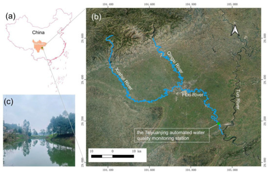
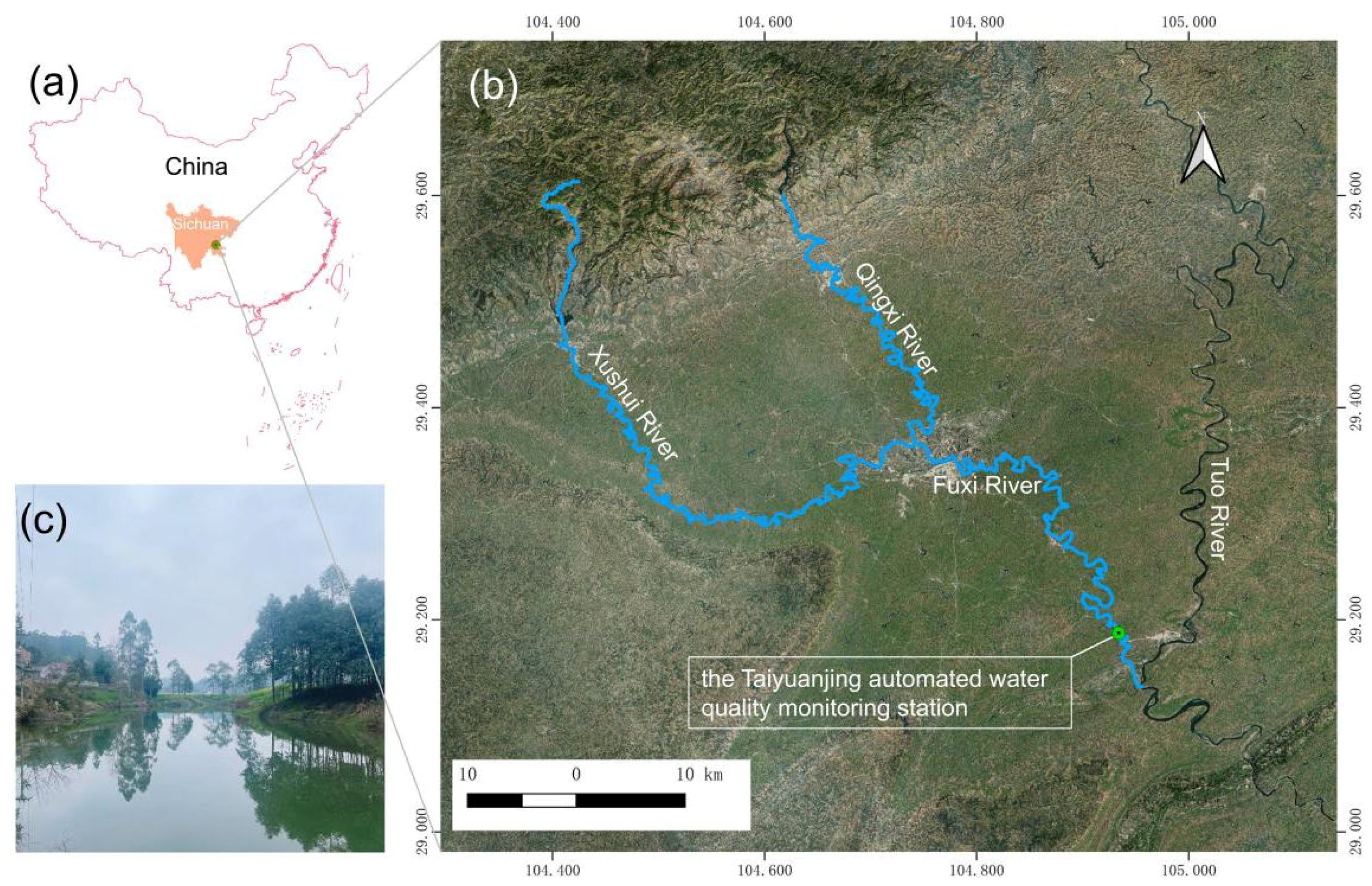
This study was conducted in the Fuxi River, a major tributary of the Tuojiang River located in Zigong City, Sichuan Province, southwestern China (Figure 1). This region has a typical subtropical humid monsoon climate and is significantly influenced by intensive urbanization and agricultural activities. To capture the fine-scale temporal dynamics of the algal proliferation, high-frequency water quality data were collected at the Taiyuanjing automated water quality monitoring station. This station is strategically positioned to reflect the integrated impact of anthropogenic nutrient loads and hydrological fluctuations on the riverine ecosystems.

The data collection extended from 18 November 2024 to 29 October 2025, nearly providing a complete annual cycle. The Taiyuanjing station operated with a 2 h temporal resolution, resulting in 12 discrete observations per day and a total of 4587 data samples over the study period.

It should be noted that the study reach of the Fuxi River is not a free-flowing natural river but is characterized as a cascade river-type reservoir. To ensure irrigation and municipal water supply, the river is regulated by multi-stage weirs and sluice gates, maintaining a quasi-constant water level of approximately 222.8 m within the study area. The average discharge is relatively low (approximately 33 m³/s), and the presence of these hydraulic structures creates extensive open water surfaces with minimal flow velocity gradients, effectively mimicking lentic (lake-like) conditions. Such stagnant or slow-flowing environments are inherently conducive to algal proliferation, which explains the recurring bloom issues in this system. Consequently, while flow velocity is a critical factor in natural lotic systems, the regulated and stabilized hydraulic state of the Fuxi River allows for a robust analysis of algal dynamics primarily through physicochemical and nutrient drivers.

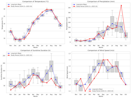
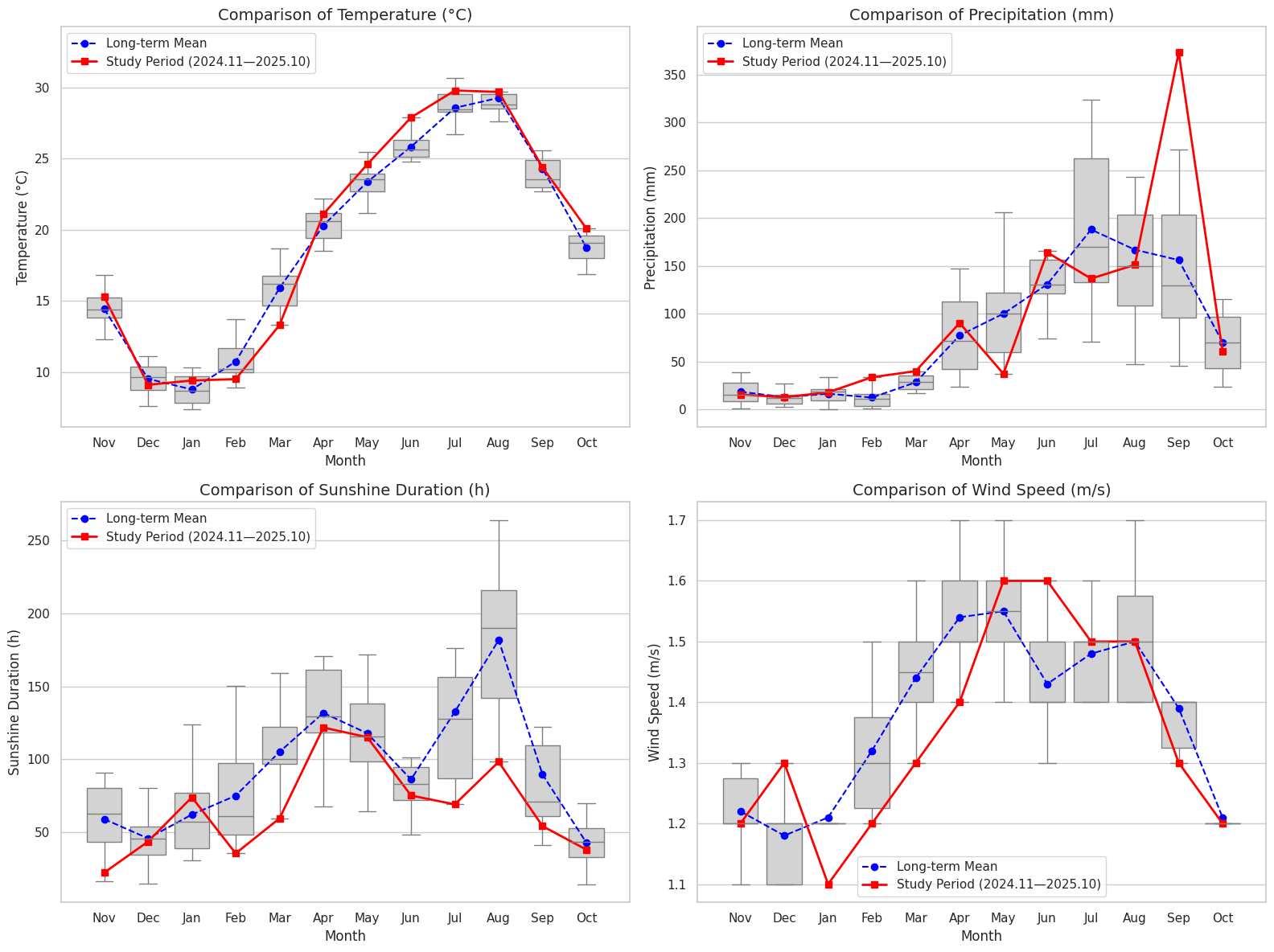
To evaluate the representativeness of the study period (November 2024–October 2025), meteorological variables were compared against long-term historical averages (2016–2025) (Figure 2). The study period exhibited notable climatic deviations: air temperatures were consistently higher, particularly in summer and autumn (e.g., 20.1 °C in October 2025 vs. the 18.75 °C average), creating a sustained thermal window for algal growth. Conversely, sunshine duration was generally attenuated (e.g., 22.2 h in November 2024 vs. the 58.92 h average), likely due to increased cloud cover associated with intensified precipitation patterns. Most significantly, September 2025 experienced extreme rainfall (372.9 mm, compared to the historical 156.15 mm), which induced pulses of allochthonous nutrient loading. Combined with slightly reduced wind speeds (averaging 1.1–1.2 m/s) that promoted water column stability, the study period provided a comprehensive range of environmental stressors. This variability ensures that the trained machine learning models are calibrated not only for average conditions but also for the extreme meteorological fluctuations that drive major algal bloom events in the Fuxi River.

Consistent with the official reporting standards of the Sichuan Provincial Environmental Monitoring Centre and to facilitate direct application in local water quality management, all water quality parameters, including Chlorophyll a, are expressed in mg/L. This ensures alignment with the regulatory assessment frameworks used in the study area.

2.2. Physicochemical Indicators and Feature Description

A comprehensive suite of water quality parameters was monitored using calibrated in situ sensors and automated analytical modules (Table 1). The water intake for the automated monitoring station was positioned at a depth of 0.5 m below the water surface, adhering to the sampling depth requirements for automated stations specified by Chinese environmental monitoring authorities. Specifically, the physical parameters, namely WT (water temperature), pH, DO (dissolved oxygen), electrical conductivity, and turbidity, along with ammonia nitrogen (NH₃-N) and total phosphorus (TP), were measured using automated analytical modules and sensors developed by ZTE Instruments (Shenzhen) Co., Ltd. (Shenzhen, China). The chemical variables, including chemical oxygen demand (Permanganate Index) (COD_Mn), were monitored using the MODEL9811 analyzer from Beijing SDL Technology Co., Ltd. (Beijing, China), while chemical oxygen demand (Dichromate Index) (COD_Cr) was measured via integrated automated modules. The taxonomic composition of the phytoplankton community was characterized through a parallel manual sampling campaign. Microscopic identification of water samples collected during the study period revealed that the community consisted of multiple taxa, including Cyanobacteria, Diatoms, Chlorophytes, Dinoflagellates, Cryptophytes, and Chrysophytes. While the automated fluorescence sensor captures the total algal density at high frequency, these manual observations confirm that the community is dominated by Cyanobacteria and Diatoms, which collectively accounted for over 75% of the total abundance on average (Figure S1). This taxonomic diversity provides the biological context for the observed fluctuations in total algal density and Chl-a concentrations.

Biological response variables, including Chl-a concentrations and algal density, were monitored in situ using a multi-wavelength fluorescence sensor integrated into the automated station (ZTE Instruments, China). This sensor operates based on the principle of selective pigment excitation; it utilizes specific light-emitting diodes (LEDs) to stimulate fluorescence from chlorophyll-a and accessory pigments (such as phycocyanin and phycoerythrin). The sensor’s internal algorithms then differentiate and quantify the equivalent cell densities of various phytoplankton groups, including Cyanobacteria, Chlorophytes, and Diatoms/Dinoflagellates, based on their unique fluorescence excitation spectra. To maintain data reliability, the sensor readings were periodically cross-validated against laboratory microscopic cell counting.

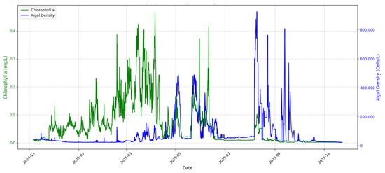
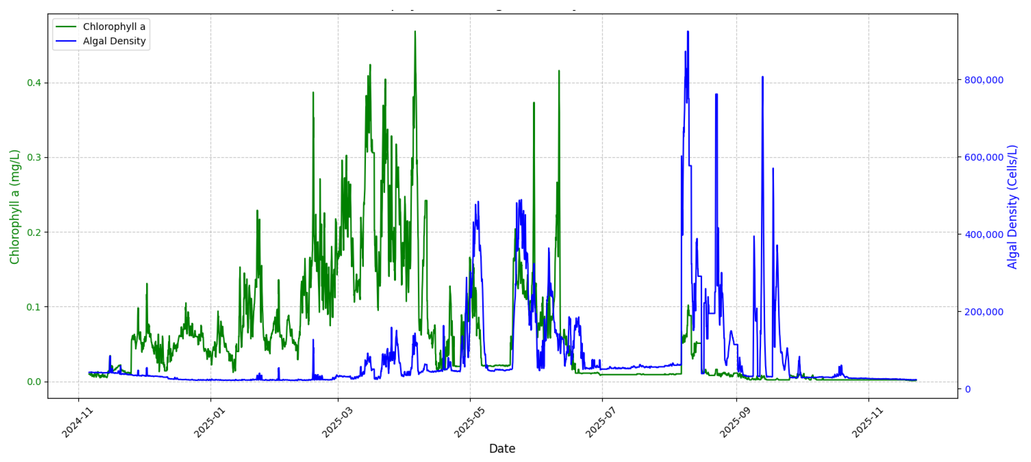
These variables were selected based on their established roles in governing phytoplankton growth dynamics. WT and DO act as context-dependent, bidirectional modulators rather than simple primary drivers: DO is both produced by photosynthesis and consumed by respiration, reflecting net metabolic balance, while WT regulates enzymatic and membrane processes governing photosynthesis and respiration [19]; importantly, blooms can also occur under ice and at low temperatures (<15 °C), where cold-adapted taxa dominate [20]. NH₃-N and TP are not universally limiting—only when external supplies fall below physiological demand do nutrients constrain growth, and above a threshold carrying capacity, saturation occurs (Liebig’s law of the minimum) [21]. Organic pollution indicators (COD_Mn, COD_Cr) were included because algal metabolism and decomposition measurably contribute to COD_Mn [22], and COD_Cr dynamics in urban rivers are closely coupled with seasonal algal proliferation [23]. In this study, Chl-a and algal density were utilized as the primary target variables (outputs) for the machine learning models to quantify the state of algal proliferation (Figure 3).

Table 1. Statistics table of the monitoring data.

Index	Units	Mean Values	Standard Deviation	Min Values	Top 25% Quantile	Top 50% Quantile	Top 75% Quantile
Water Temperature	°C	21.97	6.90	11.60	15.20	22.90	27.98
pH		8.01	0.49	5.82	7.62	7.97	8.33
Dissolved Oxygen	mg/L	9.49	4.22	0.01	6.23	8.65	12.42
Conductivity	μS/cm	898.81	196.68	459.23	694.20	962.05	1065.50
Turbidity	NTU	23.04	35.94	0.10	7.10	12.75	24.89
COD (Permanganate Index)	mg/L	4.67	0.82	3.10	4.05	4.51	5.14
Ammonia Nitrogen	mg/L	0.092	0.104	0.001	0.027	0.059	0.115
Total Phosphorus	mg/L	0.12	0.04	0.03	0.09	0.11	0.15
COD (Dichromate Index)	mg/L	21.44	8.12	11.85	16.27	18.67	24.77
Chlorophyll a	mg/L	0.0609	0.0783	0.0010	0.0090	0.0247	0.0820
Algal Density	Cells/L	80,568.28	114,369.10	20,617.00	25,878.00	41,218.25	63,409.00

Table 1. Statistics table of the monitoring data.

Index	Units	Mean Values	Standard Deviation	Min Values	Top 25% Quantile	Top 50% Quantile	Top 75% Quantile
Water Temperature	°C	21.97	6.90	11.60	15.20	22.90	27.98
pH		8.01	0.49	5.82	7.62	7.97	8.33
Dissolved Oxygen	mg/L	9.49	4.22	0.01	6.23	8.65	12.42
Conductivity	μS/cm	898.81	196.68	459.23	694.20	962.05	1065.50
Turbidity	NTU	23.04	35.94	0.10	7.10	12.75	24.89
COD (Permanganate Index)	mg/L	4.67	0.82	3.10	4.05	4.51	5.14
Ammonia Nitrogen	mg/L	0.092	0.104	0.001	0.027	0.059	0.115
Total Phosphorus	mg/L	0.12	0.04	0.03	0.09	0.11	0.15
COD (Dichromate Index)	mg/L	21.44	8.12	11.85	16.27	18.67	24.77
Chlorophyll a	mg/L	0.0609	0.0783	0.0010	0.0090	0.0247	0.0820
Algal Density	Cells/L	80,568.28	114,369.10	20,617.00	25,878.00	41,218.25	63,409.00

2.3. Data Preprocessing and Quality Control

High-frequency automated monitoring often produces datasets impacted by sensor noises, transmission interruptions, and occasional instrumental failures. To ensure the robustness and reliability of the machine learning models, a rigorous data curation protocol was implemented.

To ensure the objectivity of the data cleaning process and minimize subjective bias, a three-step automated quality control protocol was implemented. First, range checks were applied to exclude values outside the physical limits of the sensors (e.g., negative concentrations or values exceeding the maximum detection limit). Second, rate-of-change filters were employed to identify ‘spikes’—sudden fluctuations that exceed the maximum biologically or physically plausible change within a 2 h window. For instance, an abrupt increase in pH > 2.0 or a 10-fold jump in algal density within two hours was flagged as potential sensor interference rather than a real event. Third, missing values resulting from routine maintenance downtime or transmission failures were addressed using linear interpolation for short-duration gaps to preserve data continuity. Specifically, short-duration gaps with a maximum duration of 6 h (i.e., up to 3 consecutive missing data points at the 2-h sampling interval) were replaced by linear interpolations. Gaps exceeding this duration were excluded from the analysis to prevent the introduction of significant interpolation artifacts. In total, invalid data points and missing values accounted for approximately 4.2% of the raw dataset. After the rigorous data cleaning and quality control procedures, a total of 4587 valid high-frequency data points were retained for model development.

2.4. Machine Learning Model Development and Optimization

In this study, the Random Forest Regression (RFR) algorithm was employed to simulate the complex relationship between environmental drivers and algal biomass indicators (Chl-a and algal density). As an ensemble learning technique based on bagging, RFR constructs multiple decision trees during training and outputs the mean prediction of the individual trees, which effectively reduces variance and enhances model robustness against noise in high-frequency datasets. All machine learning models in this study were developed and implemented using the Python programming language (version 3.10). Specifically, the scikit-learn library was employed for data preprocessing, model training (e.g., Random Forest), and performance evaluation.

To evaluate the predictive performance and generalization capacity of the model, the preprocessed dataset was randomly partitioned into a training set (80%) and a testing set (20%) using a stochastic shuffling procedure. This split ensured that both sets encompassed a representative range of the hydrochemical conditions observed throughout the annual cycle.

A model optimization was conducted to prevent overfitting, which was a common risk when dealing with highly correlated environmental features. Hyperparameter tuning was performed through a systematic search, with a primary focus on constraining the model’s complexity. Specifically, the maximum depth of the trees (max_depth) was limited to 8, and the minimum number of samples required to be at a leaf node (min_samples_leaf) was adjusted to ensure each terminal node represents a statistically significant subset of the data. The number of estimators (trees) was set to 100 to balance between computational efficiency and stable error convergence. The predictive accuracy was quantified using the coefficient of determination (R²) and the mean squared error (MSE) across both the training and testing procedures.

The sensitivity of the machine learning models to the input environmental variables was evaluated through two distinct yet complementary lenses. First, we employed the classical Random Forest feature importance analysis, which quantifies the contribution of each parameter to the overall model accuracy by calculating the Mean Decrease in Impurity (Gini importance). Second, to provide a more granular interpretation of these sensitivities, we conducted the SHAP analysis. While the former offers a robust global ranking of variable importance consistent with established machine learning practices, the latter reveals the non-linear thresholds and directional impacts of each driver, collectively providing a comprehensive sensitivity profile of the Fuxi River’s algal dynamics.

2.5. Model Interpretability and Feature Attribution Framework

To transcend the “black-box” limitations of the RFR model and extract ecologically meaningful insights, a multi-tiered interpretability framework was implemented. Initially, global feature importance was assessed using the Gini importance (or Mean Decrease in Impurity) metric. While this provided a baseline ranking of predictor contributions, it cannot reveal the directional or non-linear nature of the relationships. The assessment of feature importance via the Gini index and the implementation of partial dependence analysis (PDA) were conducted using the scikit-learn library in Python (version 3.10). Additionally, the SHAP analysis was performed using the SHAP Python package to quantify and visualize the contribution of each environmental variable to the model’s predictions.

To address these limitations, the PDA was conducted. Partial dependence plots (PDPs) were generated to visualize the marginal effect of individual physicochemical factors on the predicted algal biomass while marginalizing the effects of other variables. This approach allowed us to identify specific response curves and non-linearities (e.g., unimodal or sigmoidal patterns) between target variables and core drivers like WT or phosphorus levels.

Finally, the SHAP method, based on coalitional game theory, was used to provide a unified and rigorous measure of feature importance. SHAP values were calculated to quantify the precise contributions of each feature to individual predictions, effectively decomposing the differences between the actual prediction and the mean prediction. This analysis focused on (1) assessing the impact of environmental features during high-concentration periods (e.g., peak bloom events); (2) comparing the feature attribution profiles across different seasons (spring vs. summer) to identify seasonal heterogeneities; and (3) identifying critical threshold effects where the marginal contribution of a feature transitions from positive to negative.

To further distill global trends from the complex interactions captured by the models, partial dependence plots (PDPs) were integrated with the SHAP analysis. While SHAP values illustrate the contribution of features for each individual observation, PDP curves represent the average marginal effect of a given predictor on the predicted Chlorophyll a or algal density, effectively highlighting the most probable functional relationships.

3. Results

3.1. Model Performance and Predictive Accuracy

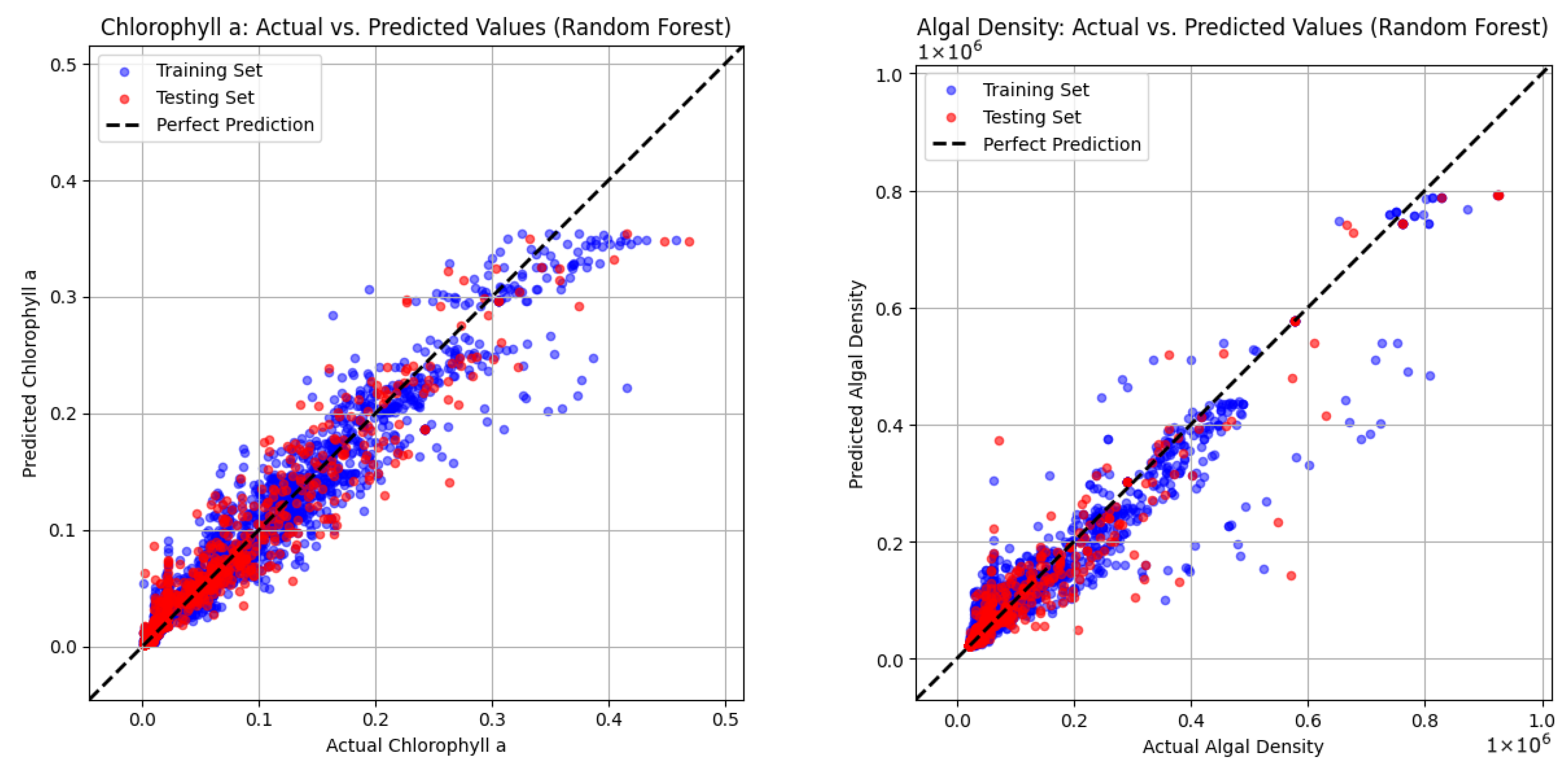
The predictive performance of the RFR models for Chl-a and algal density was rigorously evaluated using the testing dataset. The models demonstrated exceptional robustness and high fitting accuracy across the annual cycle of high-frequency observations (

Table 2. Performance evaluation metrics of machine learning models during the training phase.

Index	Target	MSE	R2
1	Chlorophyll a (Train)	0.000332668 (μg2/L2)	0.947
2	Chlorophyll a (Test)	0.00042915 (μg2/L2)	0.926
3	Algal Density (Train)	1,038,403,219 (cells2/L2)	0.921
4	Algal Density (Test)	1,238,666,970 (cells2/L2)	0.903

). For Chl-a, the RFR model achieved an R² value of 0.926 and an MSE of 0.00043 on the testing set. The model of the algal density yielded an R² value of 0.903, indicating that the ensemble learning framework successfully captured the complex non-linear dynamics inherent in the biological responses to riverine environmental stressors.

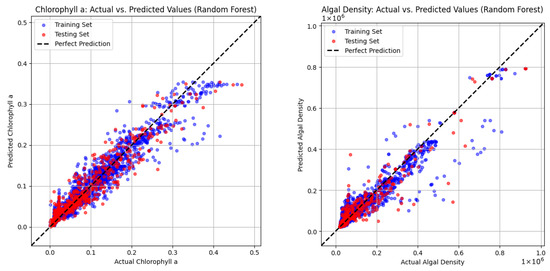
Comparisons between the observed and predicted values revealed a high degree of temporal synchrony (Figure 4). Time-series analysis showed that both the Chl-a and algal density models effectively tracked baseline fluctuations as well as rapid, transient “pulses” of algal growth. Notably, the onset and magnitude of peak proliferation events during the spring and summer seasons were simulated with high precision, demonstrating the model’s capacity to recognize the environmental triggers of algal blooms in the Fuxi River. Furthermore, the scatter regression plots illustrated a tight clustering of data points along the 1:1 identity line for both target variables. The high density of points near the diagonal across the entire concentration range confirms that the models did not suffer from significant systematic bias or heteroscedasticity, further validating the reliability of the RFR approach for high-resolution ecological forecasting.

3.2. Identification of Key Driving Factors

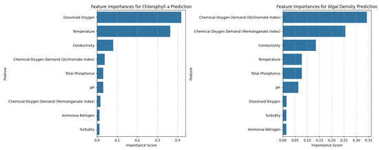
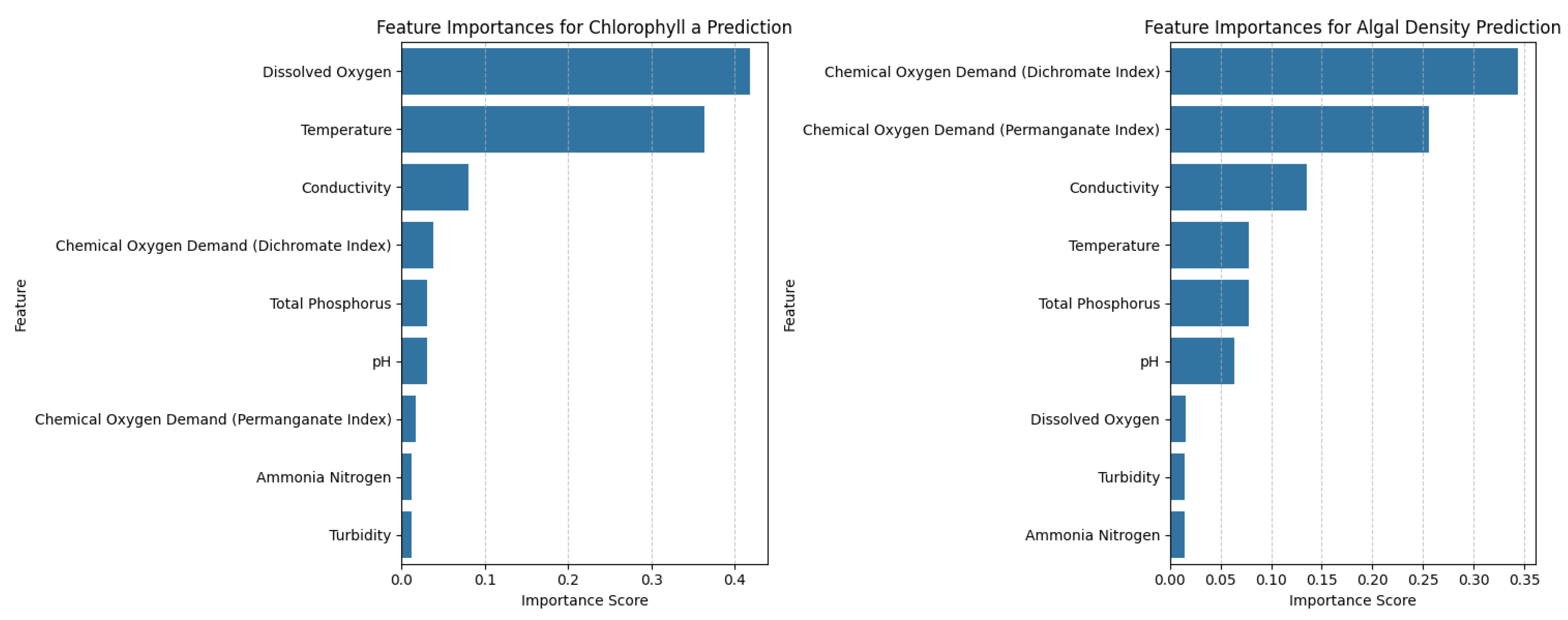
The global feature importance, derived from the Gini impurity decrease during the RF training process, provided an initial ranking of the environmental drivers governing algal dynamics in the Fuxi River (Figure 5). For the prediction of Chl-a, DO and WT emerged as the dominant explanatory variables, with importance scores of 0.42 and 0.36, respectively. This underscores the primary role of metabolic rates and thermal conditions in regulating instantaneous phytoplankton productivity. Other physicochemical factors, including pH and turbidity, exhibited considerably lower global importance, suggesting they play auxiliary roles in this human-dominated riverine system.

In contrast, the global importance profile for algal density highlighted a shift toward organic pollution indicators as primary drivers. The COD_Cr was the most significant predictor (0.20), followed closely by the COD_Mn (0.17). This discrepancy indicates that while Chl-a is acutely responsive to rapid physiological and physical environmental shifts (such as oxygenation and warming), the total algal population is more fundamentally constrained by the overall organic loading and nutrient availability within the water column.

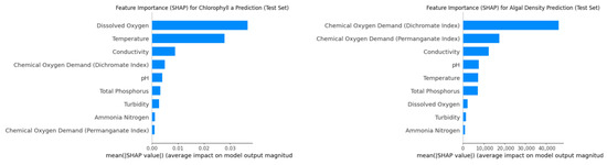
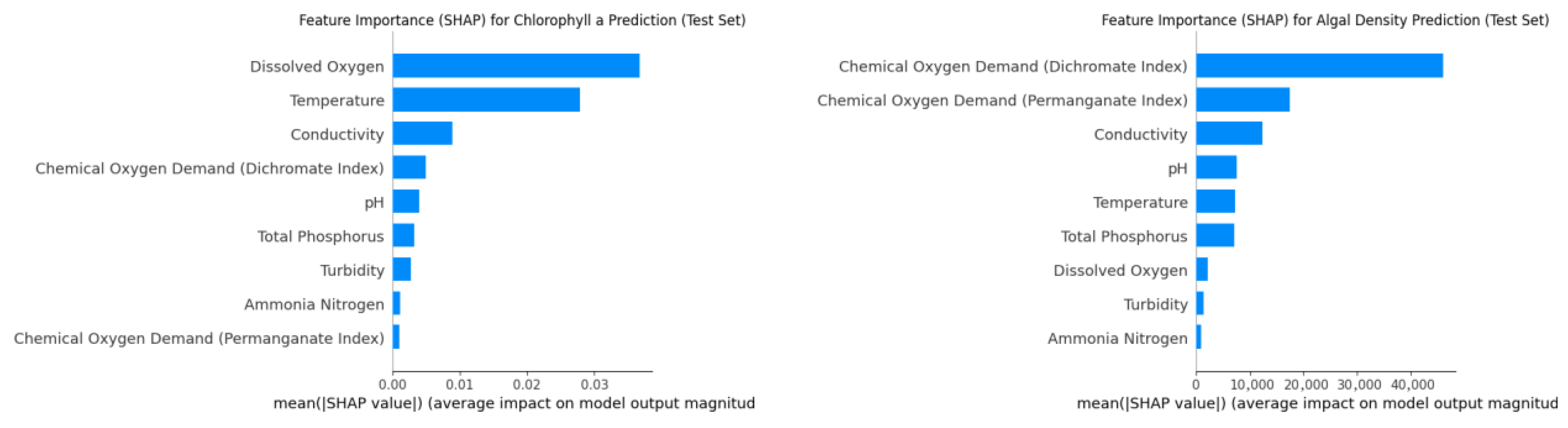
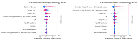
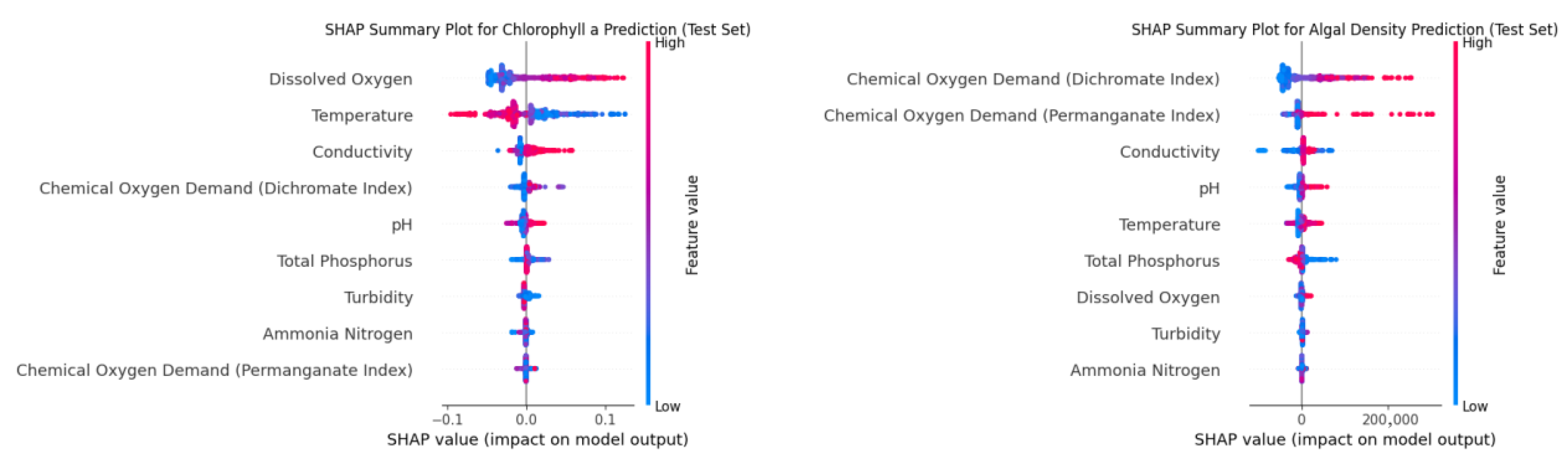
The SHAP analysis was conducted to decompose the contribution of each feature to the predicted outcomes across different concentration ranges (Figure 6). The SHAP summary plots confirmed that DO and WT maintained a consistently strong positive influence on Chl-a predictions, particularly during peak concentration events (Figure 7). For algal density, COD_Cr and COD_Mn exhibited a positive correlation with SHAP values across the majority of the observation period, confirming that elevated organic matter concentrations are prerequisites for sustained high algal densities in the Fuxi River.

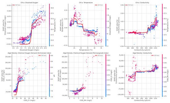
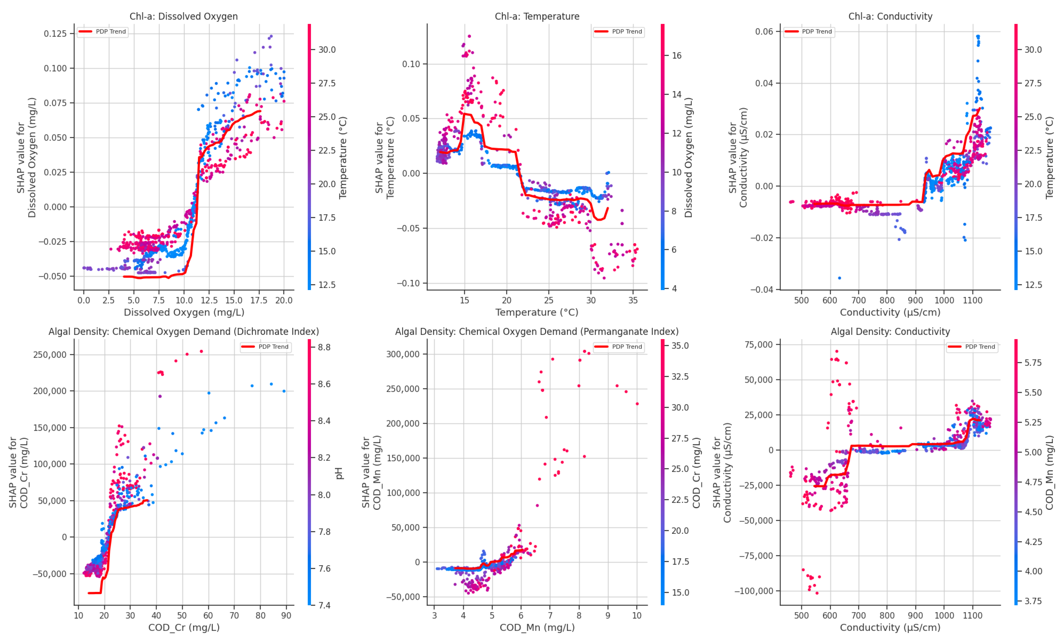
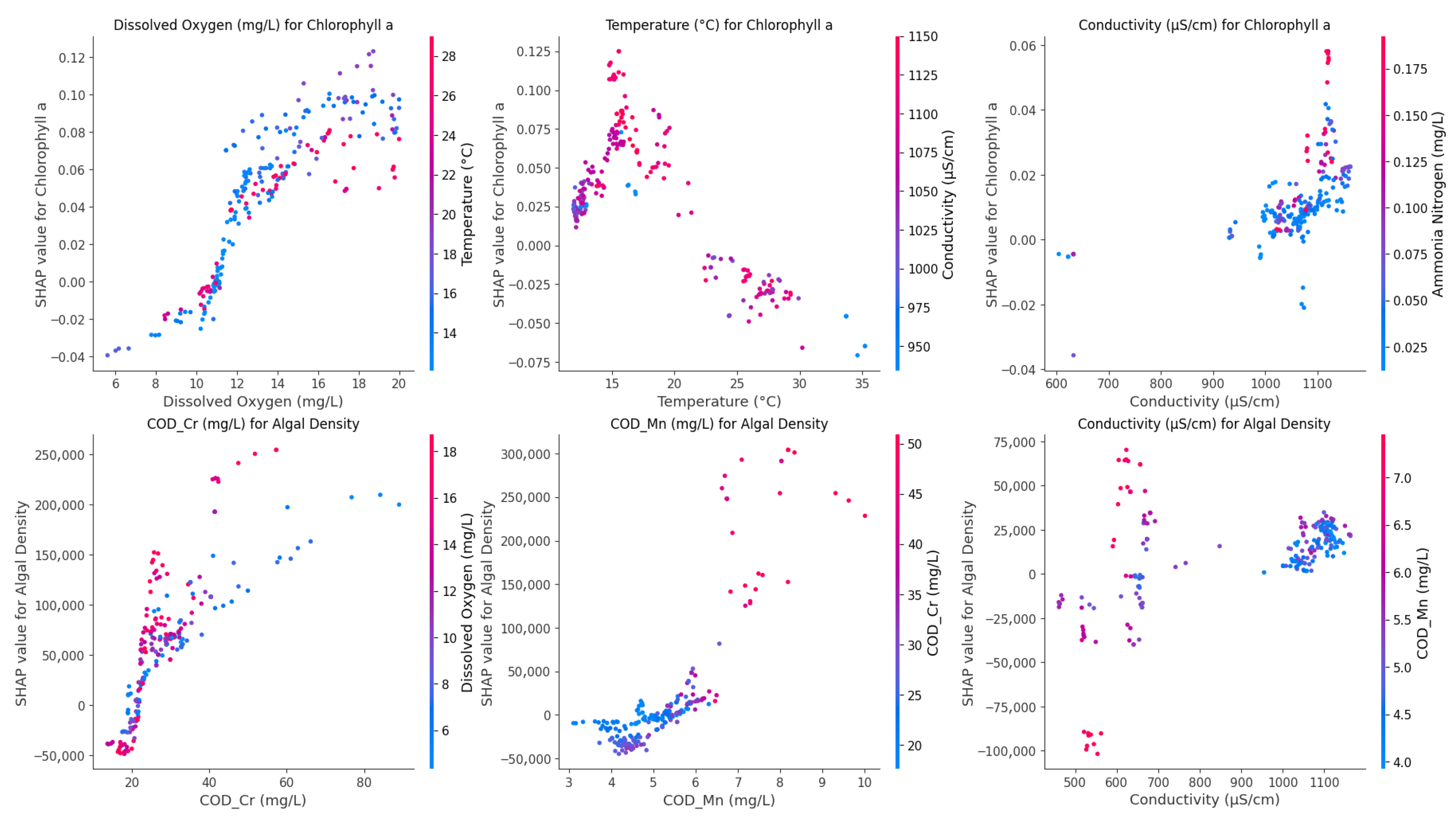
Using the PDA approach, the marginal effects of physicochemical factors on Chl-a and algal density were visualized to identify critical non-linearities. Chl-a, DO, temperature, and conductivity emerged as the dominant drivers (Figure 8). The PDP results for DO revealed a distinct non-linear growth trend; while Chl-a remained low at DO concentrations < 8 mg/L, a positive feedback mechanism became evident once concentrations surpassed the 8.74 mg/L threshold. The water temperature exhibited a seasonal threshold effect, with Chl-a increasing exponentially between 14.3 °C and 21.5 °C before entering a high-level plateau, identifying > 21.5 °C as a high-risk window for blooms. Conversely, the conductivity showed a negative correlation, where Chl-a concentrations declined in a stepwise manner with increasing ionic strength, suggesting an inhibitory effect or dilution.

The analysis of algal density highlighted COD_Cr, COD_Mn, and conductivity as the primary response variables (Figure 8). COD_Cr demonstrated a strong positive activation, with algal density responding sensitively to organic loads between 15 and 25 mg/L and peaking at 25.3 mg/L, thereby quantifying the support potential of organic pollution for algal proliferation. The COD_Mn followed a similar trajectory, driving rapid density increases within the 3.6–4.2 mg/L range. Consistent with the Chl-a findings, conductivity exhibited a “high-value inhibition” pattern, significantly suppressing the predicted algal density when exceeding 1000 μS/cm. Collectively, these thresholds—characterized as temperature > 21.5 °C, DO > 8.7 mg/L, and COD_Cr > 25 mg/L—served as robust quantitative indicators for assessing bloom risks in the study area.

3.3. Feature Dependency in High-Concentration Algal Events (Top 25% Quantile)

To further elucidate the mechanisms driving sudden algal proliferation, a subsample analysis was conducted focusing on the top 25% of high-concentration observations for both target variables (Figure 9). This approach allows for a direct comparison between baseline environmental influences and the specific drivers that triggered peak bloom events. For Chl-a concentrations in these high-value regions, the importance of DO and WT was even more pronounced than in the global analysis, with SHAP-based importance scores rising to 0.44 and 0.33, respectively. This result suggested that during peak biomass periods, the Fuxi River ecosystem became hyper-sensitive to metabolic oxygenation and thermal triggers, emphasizing that these two factors were the primary catalysts for the rapid algal growth.

A similar trend was observed for algal density within its top 25% concentration range (Figure 9). Organic pollution indicators remained the dominant drivers, with COD_Cr and the COD_Mn yielding SHAP importance scores of 0.20 and 0.18, respectively. The slight increase in the contribution of COD_Mn compared to the global model highlights the critical role of readily oxidizable organic matter in supporting high-density algal populations during bloom peaks. These findings indicate that while the general environmental structure remained consistent, the intensity of metabolic and nutrient-driven responses was significantly amplified during extreme proliferation events. Analyzing these high-value dependencies provided a more refined scientific basis for understanding the “tipping points” of algal risks in urbanized river systems.

3.4. Seasonal Dynamics of Environmental Drivers for Algal Density Prediction

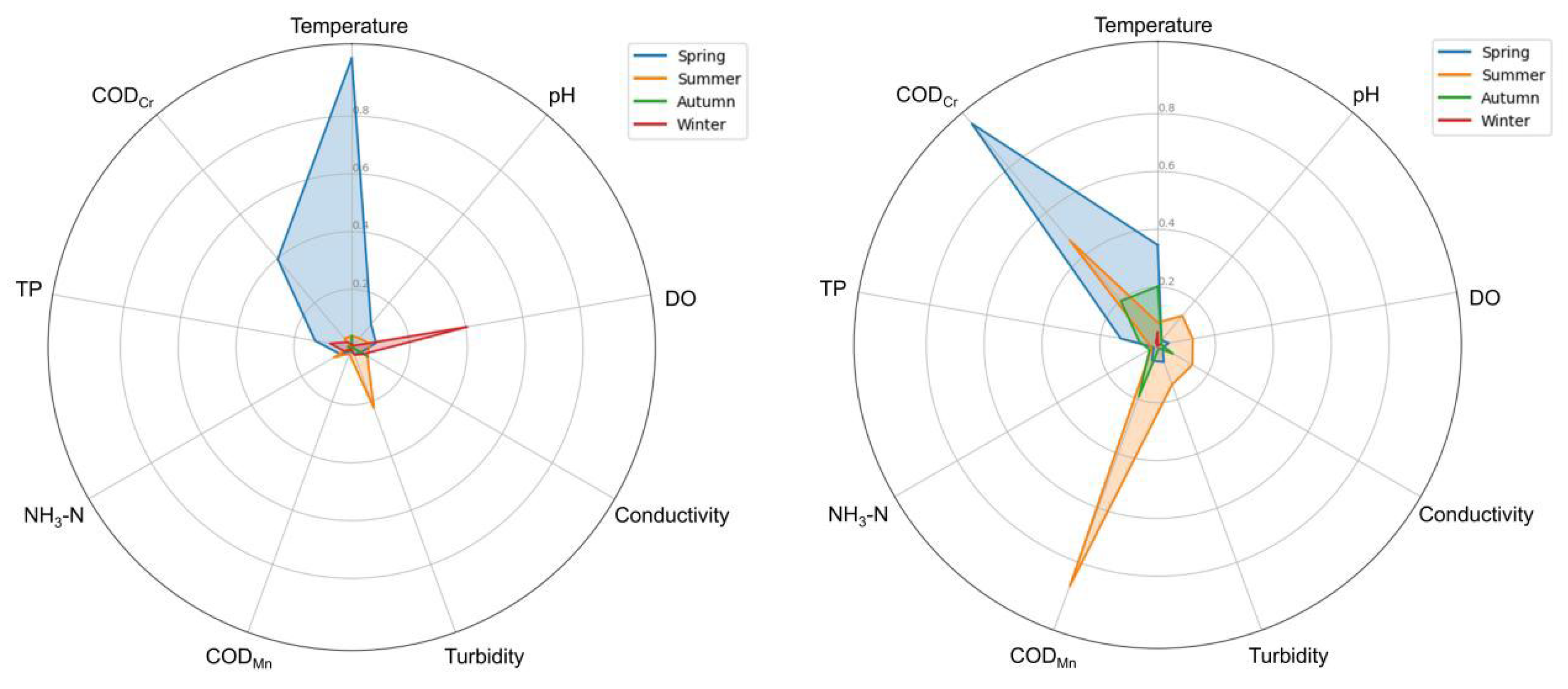
The integration of seasonal SHAP analysis revealed a profound dynamic evolution in the contributions of environmental factors across different climatic phases. For Chl-a prediction (

Table 3. The feature importance results for Chl-a using the seasonal SHAP analysis.

Index	Spring	Summer	Autumn	Winter
Turbidity	0.0021	0.018	0.00010	0.0023
Ammonia Nitrogen	0.0037	0.0056	0.00010	0.0023
COD (Dichromate Index)	0.032	0.0031	0.00010	0.0018
COD (Permanganate Index)	0.0011	0.0019	0.00020	0.00050
Conductivity	0.0029	0.0049	0.0050	0.0037
Dissolved Oxygen	0.0068	0.0051	0.00010	0.032
Water Temperature	0.079	0.0031	0.0031	0.00080
Total Phosphorus	0.010	0.00030	0.0011	0.0060
pH	0.0082	0.0033	0.00020	0.00050

), the dominant predictors changed distinctly across seasons, as DO emerged as the most critical factor in winter, whereas WT became the predominant driver during the spring transition. Similarly, for algal density (

Table 4. The feature importance results for algal density using the seasonal SHAP analysis.

Index	Spring	Summer	Autumn	Winter
Turbidity	3941	9235	770	86
Ammonia Nitrogen	1055	1532	2051	146
COD (Dichromate Index)	63,332	29,959	12,565	664
COD (Permanganate Index)	3644	56,227	12,075	315
Conductivity	1309	8738	3854	51
Dissolved Oxygen	2460	7800	793	534
Water Temperature	21,913	4904	12,827	2738
Total Phosphorus	8214	2052	4075	60
pH	1358	8369	1328	101

), a primary observation was the seasonal shift in the importance and directional influence of WT. During the spring transition, the SHAP values for WT exhibited a consistent positive trajectory as temperatures rose from winter baselines, indicating that the thermal environment acts as a primary release factor for dormant algal populations and a stimulant for initial biomass accumulation. However, this relationship underwent a significant transformation in the summer months; as temperatures reached extreme seasonal highs, the spread of SHAP values widened and frequently dipped into negative territory. This suggests that summer temperatures in the Fuxi River may surpass the optimal thermal window for certain phytoplankton taxa, leading to thermal stress and a subsequent negative contribution to the predicted algal density.

Furthermore, the seasonal influence of DO displayed complex threshold-dependent behavior (Figure 10). The SHAP analysis identified specific intervals at which the marginal impact of DO transitioned from negative to positive. In low-concentration scenarios typical of stagnant periods, SHAP values for DO were predominantly negative, whereas moderate-to-high DO levels showed strongly positive contributions to algal density forecasts. These thresholds exhibited subtle seasonal shifts, likely influenced by the varying solubility of oxygen at different temperatures.

Finally, the varying importance ranges observed across seasons underscore the shifting sensitivity of the Fuxi River ecosystem. Features with a wider spread of SHAP values in spring compared to winter reflect a greater degree of influence during the active growth season. These results indicate that the drivers of algal proliferation are not static; rather, they exist within a dynamic thermodynamic and biogeochemical feedback loop that is fundamentally shaped by seasonal climate patterns. Such high-resolution seasonal insights are essential for developing adaptive, time-specific management strategies for algal control in human-dominated riverine environments.

4. Discussion

4.1. Different Mechanisms of Physical and Chemical Drivers on Chl-a and Algal Density

The machine learning framework revealed a clear divergence in the environmental drivers of Chl-a versus algal density in the Fuxi River [24]. While Chl-a exhibited an acute sensitivity to physical metabolic drivers, specifically DO and WT, Algal Density was fundamentally constrained by organic pollution indicators such as COD_Cr and COD_Mn [25]. This discrepancy can be attributed to the distinct biological scales these two metrics represent [26]. Chl-a serves as a proxy for the instantaneous physiological and photosynthetic status of the phytoplankton community [24]. As WT directly regulates enzyme kinetics and metabolic rates, it acts as a primary “pace-setter” for pigment synthesis [27]. Similarly, the high importance of DO for Chl-a prediction (0.42 globally and 0.44 in high-concentration events) reflects the tight metabolic coupling between oxygen production and active photosynthesis [28]. In this context, DO acts as a real-time metabolic proxy that responds instantaneously to the physiological pulses of algal growth [25].

In contrast, algal density represents the accumulated standing stock or total cell count of the population, which is governed by the broader resource base and carrying capacity of the ecosystem [24]. In the human-dominated landscape of Zigong, high organic loading—characterized by COD_Cr and COD_Mn—provides a critical source of carbon and nutrients that sustain large-scale cell proliferation. The dominance of COD_Cr (0.20) and COD_Mn (0.17) in the algal density model suggests that while physical factors may trigger the rate of growth, the magnitude of the bloom (cell count) is predominantly limited by the total pool of oxidizable organic matter and associated nutrients [29]. This confirms that organic pollution indicators are not merely proxies for poor water quality but are active contributors to the sustained high-density algal populations observed in urbanized river reaches [30]. The persistence of this dominance even in high-concentration events (Top 25% quantile) emphasizes that mitigating organic pollution remains the most critical leverage point for controlling algal cell counts, whereas temperature and oxygen management are more relevant for predicting the rapid onset and physiological intensity of bloom events.

4.2. Seasonal Succession of Limiting Factors: From Thermal Triggers to Nutrient Constraints

The SHAP-based seasonal analysis underscores a fundamental shift in the limiting factors governing algal growth in the Fuxi River throughout the annual cycle. In the spring, the primary constraint is thermodynamic [31]. The consistent positive trajectory of SHAP values for WT during this period identifies thermal energy as the decisive trigger for the initiation of algal blooms [27]. During this phase, nutrient availability (represented by TP and COD) often remains at relatively high levels due to winter accumulation and early spring runoff, meaning that the ecosystem is “primed” for growth, waiting only for the temperature to cross the metabolic activation threshold [32].

However, in summer, the limiting factors undergo a significant realignment [31]. While temperature remains a high-importance feature, its marginal contribution becomes highly variable and, in some instances, inhibitory [27]. This transition suggests that once the optimal thermal window is exceeded, nutrient and organic matter supply (e.g., NH₃-N, TP, and COD) become the dominant regulators of the bloom’s peak magnitude [28]. In summer, high temperatures accelerate nutrient cycling and demand, potentially leading to transient nutrient limitation despite high overall loading [32]. The SHAP analysis revealed a wider spread of importance for organic indicators during this period, confirming that in a warm, light-saturated environment, the capacity of the river to support extreme algal densities is fundamentally governed by its anthropogenic organic burden.

Furthermore, the threshold effects observed for DO reflect a seasonal feedback loop between biological activity and the physical environment [25]. The transition of DO from a negative contributor at low concentrations to a positive one at high concentrations mirrors the shift from hypoxia-limited metabolism to high-biomass photosynthesis [28]. The seasonal shift in these thresholds implies that the Fuxi River’s “ecological tipping points” are not fixed values but are modulated by the ambient climate. From a management perspective, these findings suggest that while temperature is the primary predictor of bloom onset in the spring, the long-term prevention of summer peaks requires a year-round strategy focused on reducing the organic and nutrient carry-over from winter and spring, effectively lowering the ecosystem’s summer carrying capacity.

Finally, a notable coupling was observed between dissolved oxygen (DO) and pH (r = 0.85), with low values typically occurring simultaneously (Figure S2). These periods were characterized by high turbidity and nutrient concentrations alongside low algal biomass, suggesting that the occasional dips in DO and pH are driven by the decomposition of organic matter and high-turbidity inflows rather than nocturnal algal respiration. The reliability of these synchronized fluctuations is supported by the data validation protocols of the Sichuan Provincial Environmental Monitoring Centre, which ensures that the ‘Effective Data’ used for modeling reflects real-world water quality dynamics.

4.3. Implications for Water Environment Management and Early Warning Systems

The identification of key environmental drivers and their non-linear threshold effects provides a scientific foundation for a transition from reactive to proactive water quality management in the Fuxi River. Traditional management strategies often rely on fixed water quality standards, which fail to account for the dynamic and season-specific “risk windows” of algal proliferation [33]. By leveraging the 2 h high-frequency monitoring data and the RF-SHAP framework [34], a more responsive and precise early warning system can be established. Specifically, the identified thresholds for DO and WT can serve as real-time indicators for predicting the onset of high-concentration Chl-a events. When WT enters the activating thermal window in early spring, and DO begins its rapid positive contribution shift, managers can implement preemptive measures, such as enhanced ecological flow regulation or targeted nutrient reduction, to disrupt the bloom’s formation phase.

Moreover, the high importance of organic indicators (COD_Cr and COD_Mn) for algal density highlights the necessity of a target-specific remediation approach [29]. While physical drivers predict the timing of risk, organic loading determines the severity of the ecological impact [35]. Therefore, long-term restoration efforts in human-dominated landscapes like Zigong must prioritize reducing anthropogenic organic inputs. The SHAP analysis specifically identifies the top 25% high-concentration scenarios where the sensitivity to COD_Cr (0.20) and COD_Mn (0.18) is maximized. This precision allows for the identification of “hot moments” and “hot spots” for nutrient management, ensuring that resources are allocated to periods when the ecosystem is most vulnerable to resource-driven proliferation.

In conclusion, the integration of explainable machine learning with high-temporal-resolution monitoring offers a robust decision-support tool. By moving beyond static monitoring to dynamic, threshold-based risk assessment, water managers can better protect freshwater biodiversity and ecological health. This approach not only provides a technical solution for the Fuxi River but also offers a replicable model for other urbanized river systems globally facing similar eutrophication challenges. Implementing such a data-driven framework is a critical step toward the ecological restoration of human-dominated aquatic landscapes.

4.4. Generalizability and Context Dependence of the DO–COD Dualistic Control Framework

The finding that COD governs algal density while DO and WT drive Chl-a raises a critical question: Is this pattern exclusive to the Fuxi River? A synthesis of recent evidence suggests that this dualistic framework is not universally constant but exhibits strong context dependency, being most applicable to hypereutrophic, human-impacted water bodies with high organic loading.

First, the divergent environmental sensitivity of Chl-a versus algal density has been documented across multiple systems. A national-scale study across 57 lakes and reservoirs in China revealed that Chl-a and algal cell density (ACD) are driven by distinct environmental factors, cautioning against the blind use of Chl-a as a proxy for ACD [24]. In turbid estuarine environments, photo-acclimation under high suspended particulate matter (SPM) conditions led to elevated cellular Chl-a content, causing decoupling between cell density and Chl-a concentration [36]. In a Mediterranean eutrophic reservoir (Bidighinzu Lake, Italy), multiannual nutrient decrement resulted in increased total phytoplankton cell density but decreased mean cell volume, further demonstrating that population-level metrics (density) and physiological metrics (Chl-a) respond differently to environmental shifts [37]. These cross-system observations support our assertion that algal density is more reflective of the ecosystem’s resource and carrying capacity, rather than merely a photosynthetic proxy.

Second, regarding the dominance of COD (organic pollution) in controlling algal proliferation, multiple lines of evidence confirm that this pattern is particularly pronounced in urbanized and anthropogenically enriched watersheds. In the Chaohu Lake Basin, China, urban rivers exhibited significantly higher COD_Mn (6.30 mg/L) and Chl-a (54.88 μg/L) compared to forested rivers (4.02 mg/L and 7.18 μg/L, respectively), with urban pollutants identified as the main source of eutrophic nutrients [38]. In the Long River system (Beijing), COD_Mn was 5.98 mg/L, and the principal factors causing eutrophication included the pollution of nutritive salts and organic matter [39].

Further evidence comes from Lake Dianchi, where organic pollution-related indicators (COD, COD_Mn, and biochemical oxygen demand after 5 days)—along with TP—were identified as the primary predictors of algal biomass at most sites, despite TP dominating lake-wide control [29]. Similarly, in eutrophic plateau lakes such as Dianchi and Yilong, high densities of cyanobacteria and their metabolic products have been identified as a direct driver of persistently high COD levels, demonstrating a strong coupling between organic pollution and algal proliferation. In Yilong Lake, microbial community interactions during cyanobacteria-dominated harmful algal blooms have been shown to influence aquatic organic matter dynamics [40], while the lake’s eutrophic status and associated organic background reflect the persistence of anthropogenic organic inputs [41]. In Dianchi Lake, a distinct positive correlation between COD-Cr and Chl-a has been established, with organic substances containing nitrogen and sugars produced by algae metabolism directly contributing to COD-Cr increases; moreover, once algae cells enter the decline stage, internal organic matter released during decomposition results in a distinct COD-Cr increase, and the sediments—dominated by native organic matter predominantly derived from aquatic plants and plankton—indicate a potential long-term risk of organic pollutants being released from dead algae cells into the water column [42]. Furthermore, cyanobacterial bloom decomposition has been demonstrated to increase organic matter content in water and sediment by affecting nutrient migration and transformation, thereby driving cyanobacterial bloom development [43]. Collectively, these findings support the existence of a two-way coupling—organic pollution sustains high algal cell densities, and high cell densities in turn contribute to COD via autochthonous production and post-bloom decomposition—creating a positive feedback loop particularly pronounced in urbanized, human-impacted aquatic systems with limited hydrological exchange.

However, the universal validity of COD’s dominance is not guaranteed. The importance of organic indicators (COD) is amplified in urban river systems characterized by high input of terrigenous organic matter, slower flow velocities, and elevated nutrient backgrounds. In less enriched systems or systems where light or hydrological disturbance serves as the primary limiting factor, the relative contribution of COD to algal density diminishes. For example, studies have shown that while water diversion and hydrological adjustments can alter nutrient dynamics [41], the underlying control of algal proliferation remains highly context-dependent, varying with system-specific hydrological, chemical, and anthropogenic conditions [42]. Additionally, while COD is crucial for sustaining high standing stocks (cell counts), there is a consensus in the literature that physical factors like water temperature and dissolved oxygen remain the primary triggers for the rapid onset of physiological activity (Chl-a) [44].

In summary, our core finding—that mitigating organic pollution is vital for controlling algal cell counts—generalizes best to human-dominated, slow-flowing freshwater systems with significant external organic loading, of which the Fuxi River is a representative case. By framing our findings within this context specificity, we align with the growing recognition that the key drivers of algal blooms are not universal constants but are highly contingent on system-specific hydrological, chemical, and anthropogenic conditions.

5. Conclusions

This study demonstrated the effectiveness of integrating 2 h high-frequency water quality monitoring data with an interpretable machine learning framework (RF-SHAP) to unravel the complex drivers of algal proliferation in the human-dominated Fuxi River. The RF models exhibited exceptional predictive performance, achieving high fitting accuracy for both Chl-a and total algal density. By capturing transient biological pulses and fine-scale temporal structures that are typically overlooked by conventional monitoring programs, this high-resolution approach provides a more robust scientific basis for aquatic ecological assessment.

The distinct roles of physical metabolic drivers (WT, DO) in triggering physiological pulses and organic pollution indicators (COD_Cr and COD_Mn) in sustaining biomass standing stocks were quantified using SHAP analysis. The identification of seasonal shifts—transitioning from thermal activation in spring to nutrient/organic constraints and thermal stress in summer—along with specific threshold effects for oxygenation, underscores the non-linear nature of algal responses to environmental stressors.

Future research should focus on enhancing the spatial scalability of this framework through multi-site validation across diverse river catchments to test the universality of the identified thresholds. Furthermore, comparing the performance of ensemble methods with advanced deep learning architectures, such as Long Short-Term Memory (LSTM) networks, could further improve the modeling of long-range temporal dependencies in high-frequency datasets. Integrating these interpretable data-driven tools into real-time water management systems will be instrumental in the proactive conservation of freshwater biodiversity and the ecological restoration of anthropogenic aquatic landscapes.

References

- Sung, Y.H.; Liew, J.H.; Chan, W.S.; Fok, A.W.L.; Leung, J.; Wong, H.F.; Baker, D.M.; Bonebrake, T.C.; Dingle, C.; Dudgeon, D.; et al. Stable isotope analysis successfully identifies wild-caught individuals of threatened asian freshwater turtles in illegal trade. Glob. Ecol. Conserv. 2025, 64, e03947. [Google Scholar] [CrossRef] [Scilit]
- Faghihinia, M.; Xu, Y.; Liu, D.; Wu, N. Freshwater biodiversity at different habitats: Research hotspots with persistent and emerging themes. Ecol. Indic. 2021, 129, 107926. [Google Scholar] [CrossRef] [Scilit]
- Huisman, J.; Codd, G.A.; Paerl, H.W.; Ibelings, B.W.; Verspagen, J.M.H.; Visser, P.M. Cyanobacterial blooms. Nat. Rev. Microbiol. 2018, 16, 471–483. [Google Scholar] [CrossRef] [Scilit]
- Paerl, H.W.; Barnard, M.A. Mitigating the global expansion of harmful cyanobacterial blooms: Moving targets in a human- and climatically-altered world. Harmful Algae 2020, 96, 101845. [Google Scholar] [CrossRef] [Scilit]
- Li, T.; Zhang, Y.; Zhang, L.; Liu, Z.; Zhu, J.; Zhou, Y.; Yang, J.R. Succession of phytoplankton functional groups in a subtropical lake associated with rainfall patterns. Sci. Rep. 2025, 15, 16865. [Google Scholar] [CrossRef] [Scilit] [PubMed]
- Ho, J.C.; Michalak, A.M. Challenges in tracking harmful algal blooms: A synthesis of evidence from Lake Erie. J. Gt. Lakes Res. 2015, 41, 317–325. [Google Scholar] [CrossRef] [Scilit]
- Joshi, N.; Park, J.; Zhao, K.; Londo, A.; Khanal, S. Monitoring harmful algal blooms and water quality using sentinel-3 OLCI satellite imagery with machine learning. Remote Sens. 2024, 16, 2444. [Google Scholar] [CrossRef] [Scilit]
- Kirchner, J.W. Getting the right answers for the right reasons: Linking measurements, analyses, and models to advance the science of hydrology. Water Resour. Res. 2006, 42, W03S04. [Google Scholar] [CrossRef] [Scilit]
- Westerberg, I.K.; Wagener, T.; Coxon, G.; Mcmillan, H.K.; Castellarin, A.; Montanari, A.; Freer, J. Uncertainty in hydrological signatures for gauged and ungauged catchments. Water Resour. Res. 2016, 52, 1847–1865. [Google Scholar] [CrossRef] [Scilit]
- Zhao, W.; Li, Z.L.; Wu, H.; Tang, B.H.; Zhang, X.; Song, X.; Zhou, G. Determination of bare surface soil moisture from combined temporal evolution of land surface temperature and net surface shortwave radiation. Hydrol. Process. 2013, 27, 2825–2833. [Google Scholar] [CrossRef] [Scilit]
- Wagener, T.; Sivapalan, M.; Troch, P.A.; Mcglynn, B.L.; Harman, C.J.; Gupta, H.V.; Kumar, P.; Rao, P.S.C.; Basu, N.S.; Wilson, J.S. The future of hydrology: An evolving science for a changing world. Water Resour. Res. 2010, 46, WR008906. [Google Scholar] [CrossRef] [Scilit]
- Kim, S.; Kim, S.; Green, C.H.M.; Jeong, J. Multivariate polynomial regression modeling of total dissolved-solids in rangeland stormwater runoff in the Colorado River Basin. Environ. Modell. Softw. 2022, 157, 105523. [Google Scholar] [CrossRef] [Scilit]
- Breiman, L. Random Forests. Mach. Learn. 2001, 45, 5–32. [Google Scholar] [CrossRef] [Scilit]
- Shen, C. A transdisciplinary review of deep learning research and its relevance for water resources scientists. Water Resour. Res. 2018, 54, 8541–9707. [Google Scholar] [CrossRef] [Scilit]
- Tyralis, H.; Papacharalampous, G.; Langousis, A. A brief review of random forests for water scientists and practitioners and their recent history in water resources. Water 2019, 11, 910. [Google Scholar] [CrossRef] [Scilit]
- Olden, J.D.; Lawler, J.J.; Poff, N.L. Machine learning methods without tears: A primer for ecologists. Q. Rev. Bio. 2008, 83, 171–193. [Google Scholar] [CrossRef] [Scilit] [PubMed]
- Lundberg, S.M.; Lee, S.I. A unified approach to interpreting model predictions. In Advances in Neural Information Processing Systems 30 (NeurIPS 2017), Proceedings of the 31st Conference on Neural Information Processing Systems; Guyon, I., Luxburg, U.V., Bengio, S., Wallach, H., Fergus, R., Vishwanathan, S., Garnett, R., Eds.; Curran Associates, Inc.: Red Hook, NY, USA, 2017; pp. 4765–4774. [Google Scholar]
- Molnar, C. Interpretable Machine Learning: A Guide for Making Black Box Models Explainable, 2nd ed. Available online: https://christophm.github.io/interpretable-ml-book/ (accessed on 16 April 2026).
- Coffey, R.; Paul, M.J.; Stamp, J.; Hamilton, A.; Johnson, T. A review of water quality responses to air temperature and precipitation changes 2: Nutrients, algal blooms, sediment, pathogens. JAWRA J. Am. Water Resour. Assoc. 2019, 55, 844–868. [Google Scholar] [CrossRef] [Scilit]
- Reinl, K.L.; Harris, T.D.; North, R.L.; Almela, P.; Berger, S.A.; Bizic, M.; Burnet, S.H.; Grossart, H.P.; Ibelings, B.W.; Jakobsson, E. Blooms also like it cold. Limnol. Oceanogr. Lett. 2023, 8, 546–564. [Google Scholar] [CrossRef] [Scilit]
- Chorus, I.; Spijkerman, E. What Colin Reynolds could tell us about nutrient limitation, N: P ratios and eutrophication control. Hydrobiologia 2021, 848, 95–111. [Google Scholar] [CrossRef] [Scilit]
- Yu, H.; Zhang, J.; Yin, Z.; Liu, Z.; Chen, J.; Xu, J.; Gao, Q.; Liu, J. A method for quantifying the contribution of algal sources to CODMn in water bodies based on ecological chemometrics and its potential applications. Environ. Chem. Eng. 2024, 12, 111943. [Google Scholar] [CrossRef] [Scilit]
- Shan, X.; Li, C.G.; Li, F.M. Water quality variation of a typical urban landscape river replenished with reclaimed water. Water Cycle 2023, 4, 137–144. [Google Scholar] [CrossRef] [Scilit]
- Nong, X.; Huang, L.; Chen, L.; Wei, J.; Li, R. Distribution, relationship, and environmental driving factors of chlorophyll-a and algal cell density: A national view of China. Glob. Ecol. Conserv. 2024, 54, e03084. [Google Scholar] [CrossRef] [Scilit]
- Gao, L.; Shangguan, Y.; Sun, Z.; Shen, Q.; Zhou, L. A novel algal bloom risk assessment framework by integrating environmental factors based on explainable machine learning. Ecol. Inform. 2025, 87, 103098. [Google Scholar] [CrossRef] [Scilit]
- He, Y.; Wang, X.; Xu, F. How reliable is chlorophyll-a as algae proxy in lake environments? New insights from the perspective of n-alkanes. Sci. Total Environ. 2022, 836, 155700. [Google Scholar] [CrossRef] [Scilit] [PubMed]
- Fadel, A.; Atoui, A.; Lemaire, B.J.; Vinçon-Leite, B.; Slim, K. Environmental factors associated with phytoplankton succession in a Mediterranean reservoir with a highly fluctuating water level. Environ. Monit. Assess. 2015, 187, 633. [Google Scholar] [CrossRef] [Scilit] [PubMed]
- Wu, Y.; Xian, B.; Xiang, X.; Fang, F.; Chu, F.; Deng, X.; Fang, T. Identification of key feature variables and prediction of harmful algal blooms in a water diversion lake based on interpretable machine learning. Environ. Res. 2025, 276, 121491. [Google Scholar] [CrossRef] [Scilit] [PubMed]
- Huang, J.; Zhang, J.; Wang, N.; Hu, S.; Duan, Y. Identification of the driving factors to algal biomass in Lake Dianchi: Implications for eutrophication control. Water 2024, 16, 3485. [Google Scholar] [CrossRef] [Scilit]
- Dai, J.Y.; Wu, S.; Lv, X.; Yang, Q.; Wu, X.; Zhou, J.; Wang, F. Effect of water diversion on spatial-temporal dynamics of organic pollutants in Gonghu Bay, Lake Taihu. J. Hydroecol. 2016, 37, 39–46. [Google Scholar]
- Wen, C.C.; Huang, T.L.; Kong, C.H.; Zhang, Z.G.; Tian, P.F. Analysis of mechanism and start-up thresholds of seasonal algal blooms in a northern eutrophic stratified reservoir. Huan Jing Ke Xue 2023, 44, 1452–1464. [Google Scholar]
- Li, Y.; Huang, Y.; Ji, D.; Cheng, Y.; Nwankwegu, A.S.; Paerl, H.W.; Li, J. Storm and floods increase the duration and extent of phosphorus limitation on algal blooms in a tributary of the Three Gorges Reservoir, China. J. Hydrol. 2022, 607, 127562. [Google Scholar] [CrossRef] [Scilit]
- Busari, I.; Sahoo, D.; Harmel, R.D.; Haggard, B.E. A review of machine learning models for harmful algal bloom monitoring in freshwater systems. J. Nat. Resour. Agric. Ecosyst. 2023, 1, 63–76. [Google Scholar] [CrossRef] [Scilit]
- Demiray, B.Z.; Mermer, O.; Baydaroğlu, Ö.; Demir, I. Predicting harmful algal blooms using explainable deep learning models: A comparative study. Water 2025, 17, 676. [Google Scholar] [CrossRef] [Scilit]
- Shi, X.; Wang, L.; Chen, A.; Yu, W.; Liu, Y.; Huang, X.; Qu, D. Enhancing water quality and ecosystems of reclaimed water-replenished river: A case study of Dongsha River, Beijing, China. Sci. Total Environ. 2024, 926, 172024. [Google Scholar] [CrossRef] [Scilit]
- Jiang, Z.P.; Tong, Y.; Tong, M.; Yuan, J.; Cao, Q.; Pan, Y. The effects of suspended particulate matter, nutrient, and salinity on the growth of Amphidinium carterae under estuary environmental conditions. Front. Mar. Sci. 2021, 8, 690764. [Google Scholar] [CrossRef] [Scilit]
- Pulina, S.; Lugliè, A.; Mariani, M.A.; Sarria, M.; Sechi, N.; Padedda, B.M. Multiannual decrement of nutrient concentrations and phytoplankton cell size in a Mediterranean reservoir. Nat. Conserv. 2019, 34, 163–191. [Google Scholar] [CrossRef] [Scilit]
- Wu, L.; Liu, K.; Wang, Z.; Yang, Y.; Sang, R.; Zhu, H.; Liu, F. Temporal–spatial variations in physicochemical factors and assessing water quality condition in river–lake system of Chaohu Lake Basin, China. Sustainability 2025, 17, 2182. [Google Scholar] [CrossRef] [Scilit]
- Liu, J.; Du, G.; Wu, D.; Wu, Y.; Yang, Z.; Hua, Z. On nutritional status and blue-green algae water bloom of urban rivers and lakes in Beijing. J. Saf. Environ. 2006, 6, 5–8. [Google Scholar]
- Jin, Y.; Ren, S.; Wu, Y.; Zhang, X.; Chen, Z.; Xie, B. Microbial community structures and bacteria-Cylindrospermopsis raciborskii interactions in Yilong Lake. FEMS Microbiol. Ecol. 2024, 100, fiae048. [Google Scholar] [CrossRef] [Scilit]
- Wu, Y.; Peng, C.; Li, G.; He, F.; Huang, L.; Sun, X.; Wu, S. Integrated evaluation of the impact of water diversion on water quality index and phytoplankton assemblages of eutrophic lake: A case study of Yilong Lake. J. Environ. Manag. 2024, 357, 120707. [Google Scholar] [CrossRef] [Scilit]
- He, J.; Zhang, Y.; Wu, X.; Yang, Y.; Xu, X.; Zheng, B.; Deng, W.; Shao, Z.; Lu, L.; Wang, L.; et al. A study on the relationship between metabolism of cyanobacteria and chemical oxygen demand in Dianchi Lake, China. Water Environ. Res. 2019, 91, 1650–1660. [Google Scholar] [CrossRef] [Scilit]
- Zhang, W.; Gu, P.; Zhu, W.; Jing, C.; He, J.; Yang, X.; Zhou, L.; Zheng, Z. Effects of cyanobacterial accumulation and decomposition on the microenvironment in water and sediment. J. Soils Sediments 2020, 20, 2510–2525. [Google Scholar] [CrossRef] [Scilit]
- Yang, J.; Wang, F.; Lv, J.; Liu, Q.; Nan, F.; Xie, S.; Feng, J. Responses of freshwater algal cell density to hydrochemical variables in an urban aquatic ecosystem, northern China. Environ. Monit. Assess. 2019, 191, 29. [Google Scholar] [CrossRef] [Scilit]
Disclaimer/Publisher’s Note: The statements, opinions and data contained in all publications are solely those of the individual author(s) and contributor(s) and not of MDPI and/or the editor(s). MDPI and/or the editor(s) disclaim responsibility for any injury to people or property resulting from any ideas, methods, instructions or products referred to in the content. |
© 2026 by the authors. Licensee MDPI, Basel, Switzerland. This article is an open access article distributed under the terms and conditions of the Creative Commons Attribution (CC BY) license.