Geographically Weighted Regression Enhances Spectral Diversity–Biodiversity Relationships in Inner Mongolian Grasslands

Abstract

The spectral variation hypothesis (SVH) posits that the complexity of spectral information in remote sensing imagery can serve as a proxy for regional biodiversity. However, the relationship between spectral diversity (SD) and biodiversity differs for different environmental conditions. Previous SVH studies often overlooked these differences. We utilized species data from field surveys in Inner Mongolia and drone-derived multispectral imagery to establish a quantitative relationship between SD and biodiversity. A geographically weighted regression (GWR) model was used to describe the SD–biodiversity relationship and map the biodiversity indices in different experimental areas in Inner Mongolia, China. Spatial autocorrelation analysis revealed that both SD and biodiversity indices exhibited strong and statistically significant spatial autocorrelation in their distribution patterns. Among all spectral diversity indices, the convex hull area exhibited the best model fit with the Margalef richness index (Margalef), the coefficient of variation showed the strongest predictive performance for species richness (Richness), and the convex hull volume provided the highest explanatory power for Shannon diversity (Shannon). Predictions for Shannon achieved the lowest relative root mean square error (RRMSE = 0.17), indicating the highest predictive accuracy, whereas Richness exhibited systematic underestimation with a higher RRMSE (0.23). Compared to the commonly used linear regression model in SVH studies, the GWR model exhibited a 4.7- to 26.5-fold improvement in goodness-of-fit. Despite the relatively low R² value (≤0.59), the model yields biodiversity predictions that are broadly aligned with field observations. Our approach explicitly considers the spatial heterogeneity of the SD–biodiversity relationship. The GWR model had significantly higher fitting accuracy than the linear regression model, indicating its potential for remote sensing-based biodiversity assessments.

1. Introduction

Biodiversity reflects the stability of ecosystems and the diversity of life on Earth. It is critical to humanity’s survival and sustainable development [1,2]. Global biodiversity has declined by 2% to 11% over the past century [3]. Biodiversity loss and climate change have become the most significant threats to human well-being [4,5]. Grasslands are among the most important ecosystems for biodiversity. Approximately 49% of global grassland ecosystems have experienced degradation [6,7], resulting in biodiversity loss [8]. Comprehensive biodiversity surveys, data collection, and mapping across regions are essential to achieve global conservation goals, halt biodiversity loss, and ensure sustainable development by 2050 [9].

Field surveys of grassland biodiversity are costly, require substantial human and material resources, and disturb or damage vegetation [10]. In contrast, remote sensing technology provides significant advantages for biodiversity monitoring. It facilitates long-term, continuous, and stable time-series monitoring, making it particularly well-suited for large-scale biodiversity assessments [11]. Drones have been widely used for grassland biodiversity surveys and monitoring due to their high spatial resolution and operational flexibility [12], enabling the integration of visible, multispectral, or hyperspectral sensors. Remote sensing methods for studying grassland biodiversity include species identification, habitat suitability mapping, leaf biomass estimation, and vegetation productivity assessment [13,14,15,16]. These methods estimate community biodiversity indirectly.

The spectral variation hypothesis (SVH) postulates that biodiversity can be directly assessed through spectral information, i.e., the spectral diversity (SD) of reflected electromagnetic radiation [17] can indicate the heterogeneity of species composition and community structure, providing a biodiversity assessment method that does not require species classification [18,19,20]. Although SD shows promise as a proxy for biodiversity assessment, numerous studies have reported low, negligible, or negative correlations between SD and biodiversity, resulting in low model accuracy [21,22]. Analysis of long-term monitoring data from 192 grassland plots in southern France revealed limited predictive power, with maximum adjusted R² values of only 0.105 for all models [23]. Van Cleemput et al. analyzed pooled survey data for nine monitoring sites of the National Ecological Observatory Network (NEON), where grassland and herbaceous vegetation were the dominant cover types, and found that spectral metrics explained only 8% of biodiversity variation (R² = 0.08) [24]. However, the correlation models exhibited higher accuracy when the sites were analyzed separately. Ludwig et al. reported consistent findings, indicating substantial variability in biodiversity-SD relationships under different environmental conditions [25].

The insufficient consideration of spatial heterogeneity among ecological variables may largely account for the observed patterns. According to the first law of geography, geographic phenomena or attributes are spatially related, but spatially adjacent objects typically exhibit stronger relationships than those farther apart [26]. Several studies have demonstrated that grazing and other anthropogenic activities can markedly influence the spatial heterogeneity of plant communities [27,28]. Nevertheless, global models employed in previous studies could not fully capture the complexity of the relationship between SD and biodiversity, underscoring the necessity of accounting for local variations in SD–biodiversity dynamics in the SVH framework [24]. Geographically weighted regression (GWR) considers spatial autocorrelation and provides a more flexible and nuanced alternative to traditional global approaches [29]. It is a local linear regression technique that assesses spatial relationships between independent and dependent variables, accurately representing spatial heterogeneity. It creates regression models for each geographic location to capture local spatial patterns and variables’ heterogeneity [30,31]. Compared with traditional spatial regression approaches, GWR exhibits clear advantages in addressing spatial heterogeneity by effectively capturing spatial non-stationarity among variables and quantitatively characterizing how these relationships vary across geographic space [32].

Spatial heterogeneity serves as an indicator of habitat complexity, a factor that is broadly recognized to play a crucial role in shaping biodiversity [33]. Therefore, to address the spatial heterogeneity that has often been overlooked in previous SVH studies and to improve the modeling accuracy of the relationship between SD and biodiversity, we established a relationship between SD and biodiversity to characterize biodiversity patterns using the GWR model in Inner Mongolia, China. This approach aims to refine the SVH framework by revealing spatially varying patterns in SD–biodiversity relationships and suggests a potential way to assess grassland biodiversity indices using remote sensing, thereby supporting large-scale biodiversity monitoring and evaluation.

2. Materials and Methods

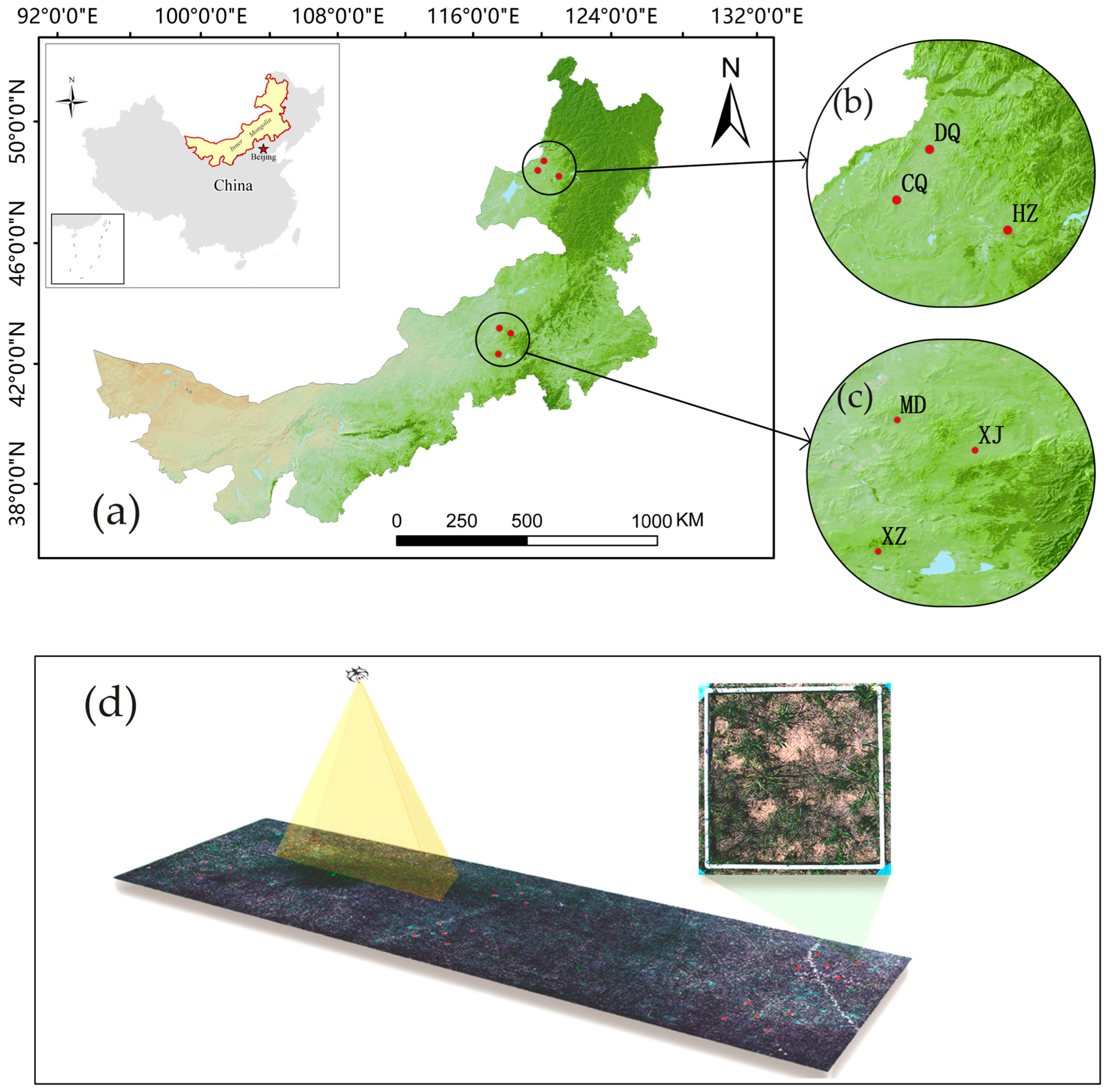
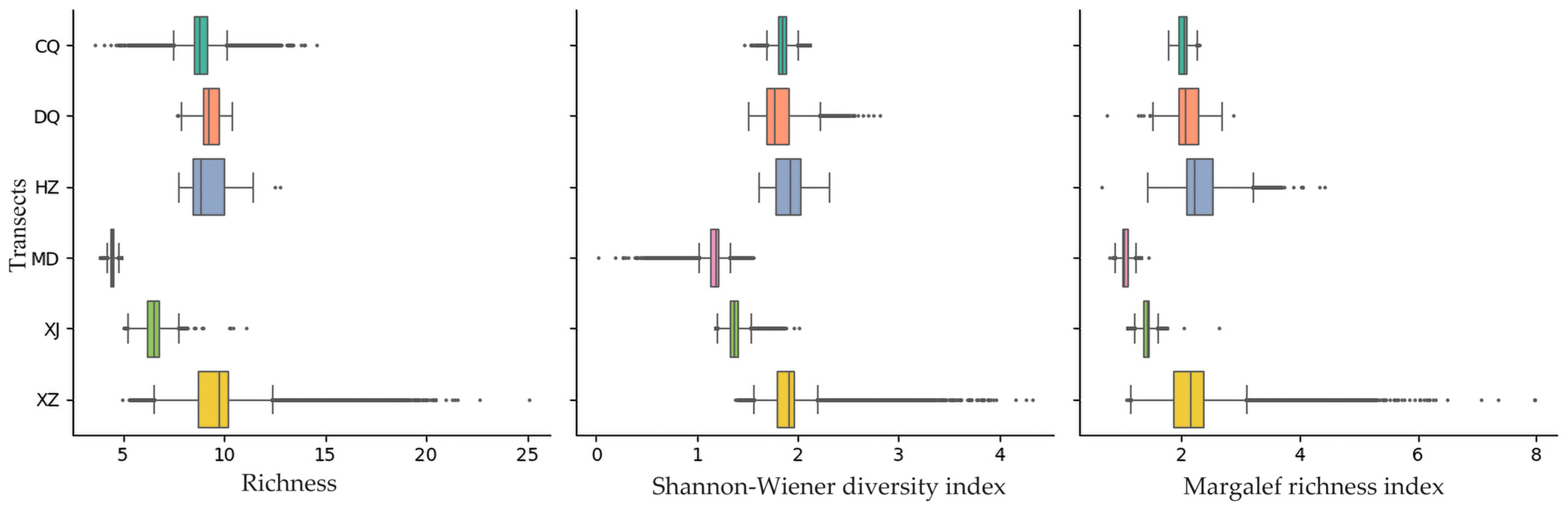
2.1. Study Area

Hulunbuir and Xilingol are situated in China’s semi-arid continental monsoon climate zone, characterized by hot, rainy summers and cold, dry winters and falls [34]. The regions have extensive grassland coverage and diverse grassland types [35,36]. They support the livelihoods of local pastoral communities and serve as ecological barriers, contributing to regional environmental stability through climate regulation, windbreak, and sand fixation [37,38]. They have high biodiversity and provide essential habitats for many wildlife species. Six experimental areas were selected to represent the ecosystem variability across these regions: four meadow steppe areas with favorable hydrothermal conditions and dense vegetation cover, and two typical steppe areas with lower precipitation and steppe vegetation (

Table 1. Information on experimental areas.

Experimental Areas	Administrative Region	Grassland Type	Coordinates	Orientation	Size (L × W, m)	Area (m2)
CQ	Hulunbuir	meadow steppe	49.57966° N, 118.93102° E	27° NE	290 × 80	23,200
DQ	Hulunbuir	meadow steppe	49.88535° N, 119.31487° E	0° NE	300 × 98	29,400
HZ	Hulunbuir	meadow steppe	49.30057° N, 119.99951° E	86° NW	490 × 67	32,830
MD	Xilingol	typical steppe	44.26940° N, 116.33487° E	15° NW	302 × 88	26,576
XZ	Xilingol	meadow steppe	43.38046° N, 116.20906° E	87° NW	317 × 96	30,432
XJ	Xilingol	typical steppe	44.06262° N, 116.86243° E	77° NW	224 × 82	18,368

, Figure 1). These areas represent the two predominant grassland types of Inner Mongolia and their key ecological characteristics. As complete grazing exclusion has not yet been fully implemented across the Inner Mongolian grasslands, the 6 experimental sites comprise fenced grasslands used exclusively for hay harvesting, without grazing, and areas under seasonal grazing management. Differences in grazing regimes may have contributed to spatial heterogeneity, but these effects were not quantified due to data limitations. All areas are privately managed grasslands enclosed by fences. Therefore, transects were positioned to capture the biodiversity gradients within each pasture, with their layout determined primarily by the orientation, length, and width of each enclosure. The transects were oriented between 27° NE and 86° NW, with areas ranging from 18,368 to 32,830 m². Detailed information on the orientation and dimensions of the six experimental areas is provided in Table 1.

2.2. Analysis Framework

We defined 3 main areas of work: data acquisition (field and drone), data processing (imagery and field data), and data analysis (global and spatial statistics) (Figure 2). In situ plant diversity surveys were conducted in Inner Mongolia, and biodiversity indices were calculated at the quadrat level. Drone flights were conducted to acquire multispectral imagery, from which the SD was derived. A global linear regression model commonly used in SVH studies and a GWR model were utilized to model the relationship between SD and biodiversity. We compared the performance of the two models to evaluate the improvement in the predictive accuracy of SD for biodiversity when spatial information was considered.

2.3. In Situ Biodiversity Survey

Vegetation surveys were conducted in the summer (from 22 July to 8 August 2024), during which time each experimental area was surveyed and contained a transect with six 30 m × 30 m sample plots. This period was selected to ensure effective observation of most species present in the region [39]. Five 1 m × 1 m quadrats were established in each plot using a five-point sampling method, resulting in 180 quadrats (due to low image quality in 2 quadrats, only 178 quadrats were used) [40]. All plant species within each 1 m × 1 m quadrat were identified in the field to the species level, and their abundances were recorded using individual counting [40]. Species presence and abundance data were documented on field sheets. Biodiversity indices are commonly used to assess regional biodiversity levels and evaluate ecosystem health and stability [41]. We utilized three diversity indices to characterize biodiversity at the quadrat scale: species richness (Richness), the Shannon–Wiener diversity index (Shannon), and the Margalef richness index (Margalef) (

Table 2. Biodiversity indices and their equations.

Biodiversity Indices	Definition	Equation
Species richness (Richness)	The number of species in the community [42].	The number of species in the community.
Shannon–Wiener diversity index (Shannon)	An index considering species richness and relative abundance [45].	$H^{\prime }=-\sum \left(P_i\mathit{ln}{P}_i\right)$, where $P_i$ is the relative abundance of the i-th species.
Margalef richness index (Margalef)	A normalized measure of species richness that incorporates abundance [46].	$Dm={\displaystyle \frac{S-1}{\mathit{ln}N}}$, where N is the total species abundance in the community.

). The indices are not restricted by a fixed range, reducing the likelihood of ecologically unrealistic predictions when modeling the relationship between biodiversity and spectral diversity. The Richness provides a straightforward measure of biodiversity [42], the Margalef accounts for variations in sampling effort and thus improves comparability across plots [43], and the Shannon integrates both species richness and evenness to offer a more comprehensive assessment of community diversity [44]. These indices form a logically integrated and complementary framework for biodiversity assessment.

2.4. Drone Multispectral Data Acquisition

High-resolution aerial imagery was collected using a DJI M300 RTK quadcopter drone, which incorporates Real-Time Kinematic (RTK) and Global Positioning System (GPS) technologies to ensure accurate georeferencing with centimeter-level precision [47]. The DJI M300 RTK is equipped with advanced flight control and motor systems and has a flight time of approximately 55 min. The fuselage is constructed from carbon fiber material to ensure stable operations under maximum wind speeds of 15 m/s. The drone has a horizontal flight speed of 23 m/s and a maximum range of 15 km. It was equipped with an AQ600 Pro multispectral camera (Yusense, Qingdao, Shandong, China) [48]. The camera has five multispectral bands and one RGB band.

Low-altitude drone flights (80 m) were conducted from July to August 2024, and imagery was acquired with 80% frontal overlap and 70% lateral overlap to ensure complete stereoscopic coverage and high-resolution data. The bands include red (central wavelength 660 nm), green (555 nm), blue (450 nm), red edge (720 nm), and near-infrared (840 nm) bands [49]. Each band has a bandwidth of 30 nm, and the spatial resolution of the images is approximately 4 cm. Image preprocessing, including geometric correction, radiometric calibration, and image mosaicking, was performed in Yusense Map (Yusense, Qingdao, Shandong, China) [49].

2.5. Spectral Diversity (SD) Metrics

SD metrics for the quadrats were calculated and employed to establish a relationship model with the biodiversity data from the field survey. We used a moving window (1 m × 1 m) to analyze the spatial variation in the SD. Non-vegetation pixels (e.g., bare soil, water, or artificial structures) were masked prior to SD computation because they can affect the SD and compromise the metric’s validity as a proxy for vegetation diversity. This step is crucial for reducing background noise and ensuring that the SD accurately describes the vegetation’s spectral variations. Threshold tests with a step size of 0.01 were conducted to determine the NDVI value for vegetation discrimination, with results remaining stable within a ±0.01 range, confirming 0.42 as the optimal threshold. Pixels with NDVI values below 0.42 were masked to remove non-vegetated areas. We applied a soil background correction to the SD calculation results because it significantly improves the accuracy of SD assessments [42].

$${SD}_{adj}={SD}_{veg}\times {\displaystyle \frac{A_{veg}}{A_{total}}}$$

(1)

where ${SD}_{adj}$ represents the adjusted spectral diversity value, ${SD}_{veg}$ refers to the spectral diversity calculated after masking out soil pixels, i.e., based solely on vegetation pixels. $A_{veg}$ denotes the area occupied by vegetation pixels within the plot, and $A_{total}$ represents the total area of the plot.

We selected 7 commonly used SD metrics to quantify SD at the quadrat scale: the coefficient of variation, spectral angle mapper, standard deviation of NDVI, spectral centroid distance, spectral information divergence, convex hull volume, and convex hull area (

Table 3. Spectral diversity metrics.

SD Metrics	Definition
Coefficient of variation	The average coefficient of variation in the band values in the quadrat [50,51].
Spectral angle mapper	The angle between the multidimensional vector of the pixel reflectance and the average spectral vector [52].
Standard deviation of NDVI	The standard deviation of the normalized difference vegetation index (NDVI) [53].
Spectral centroid distance	The average of the Euclidean distance from all spectral vectors to the mean spectral reflectance in the quadrat [54].
Spectral information divergence	The spectral information divergence compares the similarity between two pixels by measuring the probability difference between two corresponding spectral features [55].
Convex hull volume	The volume of the convex hull of the first three principal components of the pixels in the quadrat in a three-dimensional space [56,57].
Convex hull area	The area enclosed by the smallest convex polygon of the mean band reflectance and the corresponding pixel reflectance values in the quadrat [42].

) All SD metrics were expressed as the mean values at the quadrat scale.

2.6. Statistical Analysis

2.6.1. Global Linear Statistical Analysis

The in situ biodiversity indices were the response variables, and the SD metrics were the explanatory variables. The relationships between the biodiversity indices and the SD metrics were quantified using Pearson’s correlation coefficients, and statistical significance was assessed using the p-value [58]. The linear regression approach assumes linear dependence between variables, spatial stationarity of regression parameters, and homoscedasticity of residuals [59]. The coefficient of determination (R²) was used to assess the goodness-of-fit of the linear regression model [60].

2.6.2. Spatial Statistical Analysis

GWR was applied in ArcGIS 10.8 to model the relationships between biodiversity indices and SD metrics to address spatial heterogeneity. Bandwidth optimization was conducted using leave-one-out cross-validation, which minimizes prediction error. An adaptive kernel function approach was employed, with kernel bandwidth varying according to spatial density—higher densities corresponded to smaller kernel sizes and finer spatial resolution. This localized modeling approach improves our understanding of spatial variability and facilitates the prediction of biodiversity indices in unsampled regions, extending the applicability of the findings to broader spatial scales.

$$y_i=B_0(u_i,v_i)+\sum _{k=1}^m{B}_k(u_i,v_i)x_{ik}+{\epsilon }_i$$

(2)

where $y_i$ is the value of the biodiversity index at the location, $x_{ik}$ is the value of the SD metrics at location $i$, $(u_i,v_i)$ is the coordinates of $i$, $B_0(u_i,v_i)$ is the intercept of regression equation at $i$, $B_k$ (k = 1, 2, 3, …, m) is the regression coefficient, and ${\epsilon }_i$ is the random error at $i$. Each model contains one explanatory variable and one response variable. The model can be simplified as follows:

$$y_i=B_0(u_i,v_i)+B_1(u_i,v_i)x+{\epsilon }_i$$

(3)

Before applying the GWR model, a global Moran’s I analysis was conducted to assess the spatial autocorrelation of the variables. Spatial autocorrelation analysis is fundamental for identifying the spatial distribution of variables and determining whether significant spatial dependence exists. This analysis is required for the effective application of the GWR model because it determines whether the variables exhibit spatial clustering or dispersion. The GWR model could adequately capture localized variations by assessing spatial autocorrelation, improving the explanatory power and predictive accuracy of the relationships between variables. This rigorous methodological approach enhances the reliability of our findings and their applicability to spatially heterogeneous environments.

$$I={\displaystyle \frac{n{\mathsf{\Sigma }}_{\mathrm{i}=1}^n{\mathsf{\Sigma }}_{j=1}^n{W}_{ij}\left(x_i-\overline{x}\right)\left(x_j-\overline{x}\right)}{{\mathsf{\Sigma }}_{\mathrm{i}=1}^n{\mathsf{\Sigma }}_{j=1}^n{W}_{ij}{\mathsf{\Sigma }}_{\mathrm{i}=1}^n{\left(x_i-\overline{x}\right)}^2}}$$

(4)

where n is the number of spatial objects, $x_i$ is the observed value of the variable at $i$, and $W_{ij}$ is the spatial weight matrix. The range of Moran’s I is [−1, 1]. Moran’s I > 0 indicates a negative correlation, Moran’s I > 0 indicates a positive correlation, and Moran’s I = 0 denotes no spatial correlation between the spatial objects. We used the Z-score to assess spatial autocorrelation as follows:

$$Z={\displaystyle \frac{I-E\left(I\right)}{\sqrt{\mathit{var}\left(I\right)}}}$$

(5)

Moran’s I is considered statistically significant at the 99% confidence level when |Z| > 2.58 (equivalent to p < 0.01), indicating that the spatial autocorrelation of the data is not random but exhibits statistically significant spatial aggregation.

3. Results

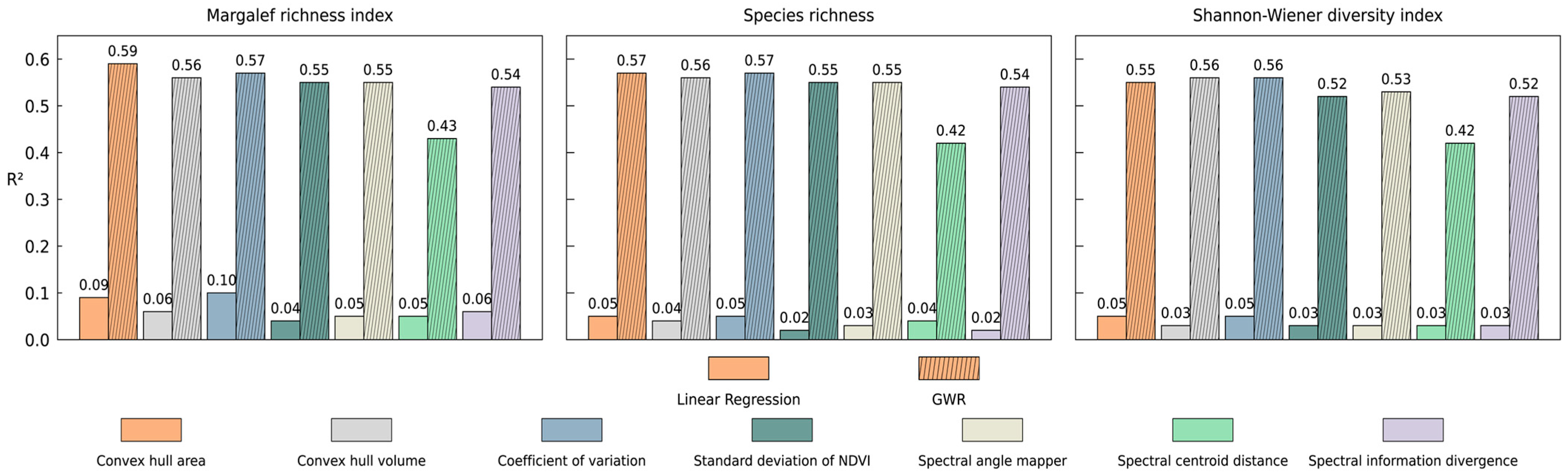
3.1. Global Linear Regression Modeling Results

Table 4. Correlation coefficients and other metrics of spectral diversity indicators for the linear regression and GWR models. Note. Significance levels: *** p < 0.001, ** p < 0.05.

Response Variables	Explanatory Variables	Pearson’s r	Linear Regression	GWR
			R2	R2	R2 Adjusted	AICc
Margalef	Convex hull area	0.29 ***	0.09	0.59	0.50	285.31
	Convex hull volume	0.25 ***	0.06	0.56	0.50	282.01
	Coefficient of variation	0.31 ***	0.10	0.57	0.50	282.14
	Standard deviation of NDVI	0.21 ***	0.04	0.55	0.48	288.48
	Spectral angle mapper	0.22 ***	0.05	0.55	0.48	287.41
	Spectral centroid distance	0.23 ***	0.05	0.43	0.40	300.91
	Spectral information divergence	0.24 ***	0.06	0.54	0.47	290.34
Richness	Convex hull area	0.21 ***	0.05	0.57	0.49	777.89
	Convex hull volume	0.20 ***	0.04	0.56	0.50	774.32
	Coefficient of variation	0.23 ***	0.05	0.57	0.50	774.41
	Standard deviation of NDVI	0.16 **	0.02	0.55	0.48	780.94
	Spectral angle mapper	0.16 **	0.03	0.55	0.48	779.66
	Spectral centroid distance	0.20 ***	0.04	0.42	0.38	797.82
	Spectral information divergence	0.16 **	0.02	0.54	0.47	783.34
Shannon	Convex hull area	0.21 ***	0.05	0.55	0.48	118.50
	Convex hull volume	0.17 **	0.03	0.56	0.50	109.55
	Coefficient of variation	0.23 ***	0.05	0.56	0.49	114.74
	Standard deviation of NDVI	0.17 **	0.03	0.52	0.45	124.68
	Spectral angle mapper	0.17 **	0.03	0.53	0.46	123.34
	Spectral centroid distance	0.18 **	0.03	0.42	0.39	132.16
	Spectral information divergence	0.18 **	0.03	0.52	0.45	125.05

presents the results of the global linear regression and the GWR. The correlation coefficient between the explanatory and response variables ranged from 0.16 to 0.31, with all correlations demonstrating statistical significance at α = 0.05 (p < 0.05), revealing statistically significant but weak positive correlations between the SD and biodiversity indices. The global linear regression models between the SD and biodiversity indices exhibited low explanatory power, with R² values ranging from 0.02 to 0.10. The coefficient of variation exhibited the strongest relationship with Margalef (R² = 0.10, p < 0.05).

3.2. Geographically Weighted Regression (GWR) Modeling Results

The spatial autocorrelation analysis (

Table 5. Spatial autocorrelation analysis results.

Variable	Moran I	Z-Score	p-Value
Species richness	0.47	14.90	0.00
Shannon–Wiener diversity index	0.47	15.00	0.00
Margalef richness index	0.47	14.98	0.00
Coefficient of variation	0.74	23.23	0.00
Spectral angle mapper	0.70	22.09	0.00
Standard deviation of NDVI	0.66	21.01	0.00
Spectral centroid distance	0.79	25.03	0.00
Spectral information divergence	0.59	18.61	0.00
Convex hull area	0.71	22.51	0.00
Convex hull volume	0.64	20.24	0.00

) demonstrates that all variables exhibited statistically significant (p < 0.01) spatial dependence, with Moran’s I ranging from 0.42 to 0.78, indicating moderate to strong autocorrelation according to conventional classification thresholds. These results confirm that the assumptions of spatial non-stationarity and dependency are met, satisfying the conditions of the GWR model. The spatial autocorrelation for all biodiversity variables suggests that conventional global regression approaches would likely produce biased estimates, justifying our choice of GWR to account for location-specific relationships in the data.

The R² and the corrected Akaike information criterion (AICc) were employed to assess the GWR models. The optimal model selection followed the established convention of maximizing the R² and minimizing the AICc values [61]. As shown in Table 4, the GWR model demonstrated a moderate goodness-of-fit (R² range: 0.42–0.59), indicating its reasonable capacity to capture SD and biodiversity. Figure 3 presents the R² values of the global linear regression model and GWR. The R² values obtained from the GWR model are significantly higher than those from the global linear regression model. The convex hull area was the most robust predictor of $Dm$ (R² = 0.59). The CV demonstrated superior performance in modeling $S$ (R² = 0.57), whereas the convex hull volume showed optimal explanatory capability for Shannon (R² = 0.56).

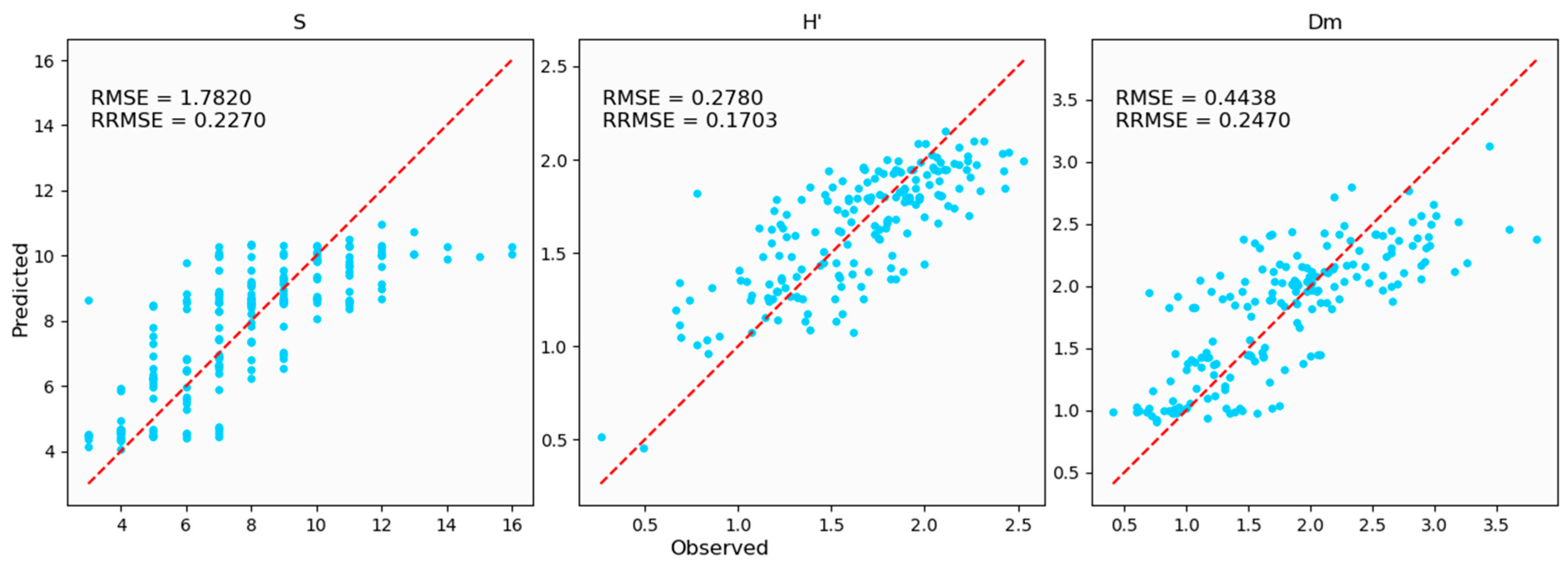
3.3. Predicted Biodiversity Indices Derived from Geographically Weighted Regression

We selected the SD metrics with the strongest explanatory power for each biodiversity index as the predictor to estimate the biodiversity in the experimental areas, with the convex hull area corresponding to $Dm$, CV to $S$, and CHA to $H^{\prime }$. Figure 4 presents the predicted biodiversity indices for the experimental areas. Due to the similar spatial distribution of the different biodiversity indices, only the predicted Margalef richness index is shown because it accurately reflects the spatial distribution of biodiversity in the study area. The biodiversity of the two typical steppe regions (MD and XJ) was lower than that of the meadow steppe regions (CQ, DQ, HZ, and XZ), with the former displaying a more uniform distribution of biodiversity. MD exhibited the lowest mean species richness and evenness, consistent with the most arid study region. In contrast, the biodiversity distribution of HZ and XZ exhibited clusters of high and low values (Figure 5). Although XZ had the highest average species richness, its biodiversity level ($H^{\prime }$) was lower than that of HZ because this metric considers species richness and evenness.

Figure 6 compares GWR predictions with observed biodiversity indicators (Richness, Shannon, and Margalef). In general, the predictions matched observations reasonably well, although some discrepancies remained (overall RRMSE ≤ 0.2470). The GWR model seemed particularly effective at capturing spatial variations in Shannon diversity (H′), achieving a relatively low prediction error (RMSE = 0.2780, RRMSE = 0.1703). Predictions for functional diversity (Margalef) were also acceptable, though slightly less precise, suggesting a moderate level of uncertainty possibly due to greater complexity in functional composition across plots. Species richness (S), however, posed the greatest challenge, especially in regions with higher biodiversity, where predictions consistently fell short of observed values (RMSE = 1.7820, RRMSE = 0.2270). The biodiversity indices predicted using SD were broadly consistent with those derived from the in situ surveys.

4. Discussion

4.1. GWR Model Improved the Performance of Predicting Biodiversity Using SD Metrics

Consistent with previous research, the fit between the SD and biodiversity indices was low for the global linear model, with a maximum R² of only 10% [23]. Inspired by Van Cleemput et al. [24], we expected the relationship between SD and biodiversity to exhibit significant spatial heterogeneity, rendering traditional global regression models inadequate for characterizing localized ecological patterns. To address this, we utilized GWR and SVH to perform a spatially explicit analysis of the biodiversity-SD relationship. Our results demonstrated that GWR substantially outperformed the global linear regression, with improvements in model fit (R²) ranging from 5.7-fold (coefficient of variation predicting Margalef, increasing from 0.07 to 0.45) to 27.5-fold (standard deviation of NDVI predicting Richness, increasing from 0.02 to 0.56) across all models (Figure 3). This robust enhancement strongly supports the hypothesized spatial non-stationarity in the relationship between SD and biodiversity. The biodiversity indices predicted using SD were largely consistent with those derived from the in situ surveys.

As shown in Figure 4, the biodiversity levels were generally higher in the eastern portion of the XZ transect than in the west, with local areas of high biodiversity values in the western section. Field observations confirmed that this area is a low-lying zone where rainfall accumulates, creating favorable conditions for high biodiversity. These findings demonstrate that integrating SD with the GWR model accurately predicted grassland biodiversity levels. Due to the distance-based weighting in the GWR model, the influence of environmental variability across different experimental areas was reduced.

4.2. Complexity of Spectral Diversity

According to our research, the GWR model had a substantially higher goodness-of-fit than the global linear regression model. However, the SD explained a maximum of only 59% of the variance in biodiversity. Thus, we discuss the underlying reasons. According to the SVH, differences in spectral responses of objects to optical sensors result in higher spectral heterogeneity in areas with higher biodiversity. SD can serve as a proxy for biodiversity [19]. However, multiple factors affect the relationship between biodiversity and SD, leading to different correlations under different conditions.

Although high biodiversity typically corresponded to high SD in this study, we observed instances where the relationship was inverted, with higher biodiversity related to lower SD (negative local coefficients). This phenomenon has also been reported in prior studies, indicating it may reflect an underlying ecological pattern rather than a coincidental occurrence [22,62]. Some studies attributed this pattern to the limited spectral information used in the analysis, suggesting that higher-resolution hyperspectral data may alleviate this effect. However, Rossi et al. [22] found that total biomass and other confounding factors of the community were the principal drivers of this phenomenon, regardless of the number of spectral bands. The complex vertical structure of vegetation communities may be a key contributing factor [63]. Vegetation communities have a three-dimensional structure and multiple layers. In plant communities with complex vertical stratification, taller vegetation can obscure shorter plants, limiting the ability of remote sensing imagery to capture spectral information from lower canopy layers. This canopy occlusion effect prevents the spectral signals of lower-layer vegetation from being adequately captured by remotely sensed imagery, thereby limiting the potential of SD as an effective proxy for biodiversity in structurally complex ecosystems. Consequently, communities with inherently high biodiversity may still exhibit relatively low spectral diversity [64,65]. The spectral centroid distance’s relatively low performance (R² = 0.42) may result from its sensitivity to vertical occlusion, with overstory vegetation masking understory spectral variation in densely layered communities [63]. Emerging 3D reconstruction technologies, such as structure-from-motion photogrammetry, enable accurate prediction of biodiversity by capturing vegetation height, volume, and other structural parameters. These methods hold great promise for advancing biodiversity research [66].

During the flowering stage, flowers exhibit spectral reflectance patterns distinct from those of leaves [67], introducing potential bias when using spectral diversity to estimate species diversity [68]. Empirical evidence suggests that phenological phenomena, such as flowering and leaf senescence, can diminish the reliability of SD as a proxy for biodiversity by introducing transient spectral variations that obscure the underlying species composition of vegetation communities [69,70]. In addition, variations in water content and leaf biomass across different phenological stages can lead to distinct differences in spectral reflectance, which are detectable in remote sensing imagery [71]. Consequently, it is imperative to account for vertical vegetation stratification and phenological variability in analytical frameworks to improve the robustness and applicability of SD-based remote sensing methods for biodiversity monitoring.

However, even when the aforementioned factors are taken into account, spectral diversity alone may not adequately capture the complexity of biodiversity patterns, and its use as a sole proxy for species diversity may lead to less reliable estimations [20]. These findings highlight the potential importance of incorporating additional environmental variables, such as climate, topography, and grazing intensity, into SVH-based research frameworks to improve the accuracy and ecological relevance of ground-level biodiversity assessments.

4.3. Future Work

Field biodiversity surveys, drone remote sensing technology, and geographic information technology were combined in this study for biodiversity mapping. Future research can integrate a broader range and a larger sample size of ground survey data with drone remote sensing technology. Incorporating satellite remote sensing data could serve as an integrated biodiversity monitoring framework, facilitating large-scale biodiversity mapping.

Many studies have demonstrated that SD could be used as a proxy for biodiversity [72,73]. However, some research limitations remain. The SVH focuses on intra-community spectral variation but disregards differences at the leaf level. Species composition, non-vegetation factors (e.g., soil, sensor characteristics, and atmospheric conditions), and the vegetation’s biochemical properties, including leaf biomass, leaf structure, chlorophyll content, and phenological stage, affect the spectral reflectance captured by optical imagery [50,74,75]. These factors introduce additional sources of spectral variation, complicating the use of SD as a biodiversity proxy. With the rapid advancement of deep learning techniques, the development of plant segmentation algorithms has provided new opportunities for spectral analysis at the plant level [76]. Individual plants can be used as analytical units in sparse vegetation communities. Their spectral characteristics can be quantified by calculating the mean spectral reflectance of the canopy pixels. This approach can be integrated with SVH to improve the assessment of spectral heterogeneity within communities while mitigating the confounding effects of intra-individual spectral variation. Moreover, the timing of image acquisition and field sampling must be accounted for to minimize seasonal biases. The geographically and temporally weighted regression (GTWR) model accounts for both spatial and temporal non-stationarity, making it potentially more suitable than traditional GWR for large-scale and long-term biodiversity monitoring. Future work will consider applying GTWR to the SVH framework to test its applicability and to provide a methodological reference for broad-scale biodiversity assessment [77].

5. Conclusions

Spatial autocorrelation analysis indicated that both SD and biodiversity indices exhibited significant spatial autocorrelation in their spatial distributions, justifying the application of the GWR model. Incorporating spatial non-stationarity through GWR, as opposed to using conventional global linear regression, significantly improves model performance and strengthens the explanatory power of SD for biodiversity spatial patterns. The resulting predictions broadly match field observations. These findings enrich and extend the theoretical framework of the SVH. GWR enhances the spatial scalability of the SVH in heterogeneous grasslands, although vertical occlusion and phenological variation remain important challenges, indicating a need to integrate 3D remote sensing and temporal modeling approaches. Future research could benefit from integrating large-scale field survey datasets with time-series remote sensing data, employing modeling frameworks incorporating both spatial and temporal dimensions to enhance understanding of biodiversity dynamics. Image resolution and spectral resolution influence the ability of SD to characterize biodiversity. Future research should identify the optimal pixel size for SVH studies, and in-depth analyses, including mechanistic investigations, should be conducted to determine spectral bands most sensitive to plant diversity.

References

1. Balmford, A.; Gaston, K.J. Why biodiversity surveys are good value. Nature 1999, 398, 204–205. [Google Scholar] [CrossRef]
2. Wagg, C.; Roscher, C.; Weigelt, A.; Vogel, A.; Ebeling, A.; De Luca, E.; Roeder, A.; Kleinspehn, C.; Temperton, V.M.; Meyer, S.T.; et al. Biodiversity–stability relationships strengthen over time in a long-term grassland experiment. Nat. Commun. 2022, 13, 7752. [Google Scholar] [CrossRef]
3. Pereira, H.M.; Martins, I.S.; Rosa, I.M.D.; Kim, H.; Leadley, P.; Popp, A.; Van Vuuren, D.P.; Hurtt, G.; Quoss, L.; Arneth, A.; et al. Global trends and scenarios for terrestrial biodiversity and ecosystem services from 1900 to 2050. Science 2024, 384, 458–465. [Google Scholar] [CrossRef]
4. Bawa, K.S.; Sengupta, A.; Chavan, V.; Chellam, R.; Ganesan, R.; Krishnaswamy, J.; Mathur, V.B.; Nawn, N.; Olsson, S.B.; Pandit, N.; et al. Securing biodiversity, securing our future: A national mission on biodiversity and human well-being for India. Biol. Conserv. 2021, 253, 108867. [Google Scholar] [CrossRef]
5. Xu, W.; Xiao, Y.; Zhang, J.; Yang, W.; Zhang, L.; Hull, V.; Wang, Z.; Zheng, H.; Liu, J.; Polasky, S.; et al. Strengthening protected areas for biodiversity and ecosystem services in China. Proc. Natl. Acad. Sci. USA 2017, 114, 1601–1606. [Google Scholar] [CrossRef]
6. Bardgett, R.D.; Bullock, J.M.; Lavorel, S.; Manning, P.; Schaffner, U.; Ostle, N.; Chomel, M.; Durigan, G.; Fry, E.L.; Johnson, D.; et al. Combatting global grassland degradation. Nat. Rev. Earth Environ. 2021, 2, 720–735. [Google Scholar] [CrossRef]
7. Gang, C.; Zhou, W.; Chen, Y.; Wang, Z.; Sun, Z.; Li, J.; Qi, J.; Odeh, I. Quantitative assessment of the contributions of climate change and human activities on global grassland degradation. Environ. Earth Sci. 2014, 72, 4273–4282. [Google Scholar] [CrossRef]
8. Petermann, J.S.; Buzhdygan, O.Y. Grassland biodiversity. Curr. Biol. 2021, 31, R1195–R1201. [Google Scholar] [CrossRef]
9. Joly, C.A. The kunming-montréal global biodiversity framework. Biota Neotropica 2022, 22, e2022e001. [Google Scholar] [CrossRef]
10. Wang, R.; Gamon, J.A. Remote sensing of terrestrial plant biodiversity. Remote Sens. Environ. 2019, 231, 111218. [Google Scholar] [CrossRef]
11. Nagendra, H. Using remote sensing to assess biodiversity. Int. J. Remote Sens. 2001, 22, 2377–2400. [Google Scholar] [CrossRef]
12. Lyu, X.; Li, X.; Dang, D.; Dou, H.; Wang, K.; Lou, A. Unmanned aerial vehicle (UAV) remote sensing in grassland ecosystem monitoring: A systematic review. Remote Sens. 2022, 14, 1096. [Google Scholar] [CrossRef]
13. Boykin, K.G.; Kepner, W.G.; Bradford, D.F.; Guy, R.K.; Kopp, D.A.; Leimer, A.K.; Samson, E.A.; East, N.F.; Neale, A.C.; Gergely, K.J. A national approach for mapping and quantifying habitat-based biodiversity metrics across multiple spatial scales. Ecol. Indic. 2013, 33, 139–147. [Google Scholar] [CrossRef]
14. Brun, P.; Zimmermann, N.E.; Graham, C.H.; Lavergne, S.; Pellissier, L.; Münkemüller, T.; Thuiller, W. The productivity-biodiversity relationship varies across diversity dimensions. Nat. Commun. 2019, 10, 5691. [Google Scholar] [CrossRef]
15. Huang, Z.; Bai, Y.; Alatalo, J.M.; Yang, Z. Mapping biodiversity conservation priorities for protected areas: A case study in xishuangbanna tropical area, China. Biol. Conserv. 2020, 249, 108741. [Google Scholar] [CrossRef]
16. Vaglio Laurin, G.; Puletti, N.; Chen, Q.; Corona, P.; Papale, D.; Valentini, R. Above ground biomass and tree species richness estimation with airborne lidar in tropical ghana forests. Int. J. Appl. Earth Obs. Geoinf. 2016, 52, 371–379. [Google Scholar] [CrossRef]
17. Fassnacht, F.E.; Müllerová, J.; Conti, L.; Malavasi, M.; Schmidtlein, S. About the link between biodiversity and spectral variation. Appl. Veg. Sci. 2022, 25, e12643. [Google Scholar] [CrossRef]
18. Fu, Y.; Yao, Y.; Wang, L.; Yi, H.; Shan, Y. How Spatial Resolution Mediates Canopy Spectral Diversity as a Proxy for Marsh Plant Diversity. Ecol. Inf. 2025, 90, 103253. [Google Scholar] [CrossRef]
19. Rocchini, D.; Chiarucci, A.; Loiselle, S.A. Testing the spectral variation hypothesis by using satellite multispectral images. Acta Oecologica 2004, 26, 117–120. [Google Scholar] [CrossRef]
20. Schmidtlein, S.; Fassnacht, F.E. The spectral variability hypothesis does not hold across landscapes. Remote Sens. Environ. 2017, 192, 114–125. [Google Scholar] [CrossRef]
21. Imran, H.A.; Gianelle, D.; Scotton, M.; Rocchini, D.; Dalponte, M.; Macolino, S.; Sakowska, K.; Pornaro, C.; Vescovo, L. Potential and limitations of grasslands α-diversity prediction using fine-scale hyperspectral imagery. Remote Sens. 2021, 13, 2649. [Google Scholar] [CrossRef]
22. Rossi, C.; Kneubühler, M.; Schütz, M.; Schaepman, M.E.; Haller, R.M.; Risch, A.C. Spatial resolution, spectral metrics and biomass are key aspects in estimating plant species richness from spectral diversity in species-rich grasslands. Remote Sens. Ecol. Conserv. 2022, 8, 297–314. [Google Scholar] [CrossRef]
23. Lopes, M.; Fauvel, M.; Ouin, A.; Girard, S. Spectro-temporal heterogeneity measures from dense high spatial resolution satellite image time series: Application to grassland species diversity estimation. Remote Sens. 2017, 9, 993. [Google Scholar] [CrossRef]
24. Van Cleemput, E.; Adler, P.; Suding, K.N. Making remote sense of biodiversity: What grassland characteristics make spectral diversity a good proxy for taxonomic diversity? Glob. Ecol. Biogeogr. 2023, 32, 2177–2188. [Google Scholar] [CrossRef]
25. Ludwig, A.; Doktor, D.; Feilhauer, H. Is spectral pixel-to-pixel variation a reliable indicator of grassland biodiversity? A systematic assessment of the spectral variation hypothesis using spatial simulation experiments. Remote Sens. Environ. 2024, 302, 113988. [Google Scholar] [CrossRef]
26. Klippel, A.; Hardisty, F.; Li, R. Interpreting spatial patterns: An inquiry into formal and cognitive aspects of tobler’s first law of geography. Ann. Assoc. Am. Geogr. 2011, 101, 1011–1031. [Google Scholar] [CrossRef]
27. Wang, Z.; Meng, P.; Wang, Z.; Lv, S.; Han, G.; Hou, D.; Wang, J.; Wang, H.; Zhu, A. Spatial distribution of shrubs and perennial plants under grazing disturbance in the desert steppe of inner mongolia. Glob. Ecol. Conserv. 2024, 54, e03193. [Google Scholar] [CrossRef]
28. Adler, P.; Raff, D.; Lauenroth, W. The effect of grazing on the spatial heterogeneity of vegetation. Oecologia 2001, 128, 465–479. [Google Scholar] [CrossRef]
29. Brunsdon, C.; Fotheringham, A.S.; Charlton, M. Geographically weighted summary statistics—A framework for localised exploratory data analysis. Comput. Environ. Urban Syst. 2002, 26, 501–524. [Google Scholar] [CrossRef]
30. Brunsdon, C.; Fotheringham, A.S.; Charlton, M.E. Geographically weighted regression: A method for exploring spatial nonstationarity. Geogr. Anal. 1996, 28, 281–298. [Google Scholar] [CrossRef]
31. Zhu, C.; Zhang, X.; Zhou, M.; He, S.; Gan, M.; Yang, L.; Wang, K. Impacts of urbanization and landscape pattern on habitat quality using OLS and GWR models in hangzhou, China. Ecol. Indic. 2020, 117, 106654. [Google Scholar] [CrossRef]
32. Gao, C.; Feng, Y.; Tong, X.; Lei, Z.; Chen, S.; Zhai, S. Modeling urban growth using spatially heterogeneous cellular automata models: Comparison of spatial lag, spatial error and GWR. Comput. Environ. Urban Syst. 2020, 81, 101459. [Google Scholar] [CrossRef]
33. Loke, L.H.L.; Chisholm, R.A. Measuring habitat complexity and spatial heterogeneity in ecology. Ecol. Lett. 2022, 25, 2269–2288. [Google Scholar] [CrossRef]
34. Weng, C.; Bai, Y.; Chen, B.; Hu, Y.; Shu, J.; Chen, Q.; Wang, P. Assessing the vulnerability to climate change of a semi-arid pastoral social–ecological system: A case study in hulunbuir, China. Ecol. Inform. 2023, 76, 102139. [Google Scholar] [CrossRef]
35. Na, R.; Du, H.; Na, L.; Shan, Y.; He, H.S.; Wu, Z.; Zong, S.; Yang, Y.; Huang, L. Spatiotemporal changes in the aeolian desertification of hulunbuir grassland and its driving factors in China during 1980–2015. Catena 2019, 182, 104123. [Google Scholar] [CrossRef]
36. Sun, B.; Li, Z.; Gao, Z.; Guo, Z.; Wang, B.; Hu, X.; Bai, L. Grassland degradation and restoration monitoring and driving forces analysis based on long time-series remote sensing data in xilin gol league. Acta Ecol. Sin. 2017, 37, 219–228. [Google Scholar] [CrossRef]
37. Li, X.; Lyu, X.; Dou, H.; Dang, D.; Li, S.; Li, X.; Li, M.; Xuan, X. Strengthening grazing pressure management to improve grassland ecosystem services. Glob. Ecol. Conserv. 2021, 31, e01782. [Google Scholar] [CrossRef]
38. Zhang, Y.; Chen, X.; Zhang, Y.; Wang, B. Quantitative contribution of climate change and vegetation restoration to ecosystem services in the Inner Mongolia under ecological restoration projects. Ecol. Indic. 2025, 171, 113240. [Google Scholar] [CrossRef]
39. Li, Z.; Ma, W.; Liang, C.; Liu, Z.; Wang, W.; Wang, L. Long-term vegetation dynamics driven by climatic variations in the inner mongolia grassland: Findings from 30-year monitoring. Landsc. Ecol. 2015, 30, 1701–1711. [Google Scholar] [CrossRef]
40. Jing-yun, F.; Xiang-ping, W.; Ze-hao, S.; Zhi-yao, T.; Jin-sheng, H.; Dan, Y.; Yuan, J.; Zhi-heng, W.; Cheng-yang, Z.; Jiang-ling, Z.; et al. Methods and protocols for plant community inventory. Biodivers. Sci. 2009, 17, 533. [Google Scholar] [CrossRef]
41. Izsák, J.; Papp, L. A link between ecological diversity indices and measures of biodiversity. Ecol. Model. 2000, 130, 151–156. [Google Scholar] [CrossRef]
42. Gholizadeh, H.; Gamon, J.A.; Zygielbaum, A.I.; Wang, R.; Schweiger, A.K.; Cavender-Bares, J. Remote sensing of biodiversity: Soil correction and data dimension reduction methods improve assessment of α-diversity (species richness) in prairie ecosystems. Remote Sens. Environ. 2018, 206, 240–253. [Google Scholar] [CrossRef]
43. Mulya, H.; Santosa, Y.; Hilwan, I. Comparison of four species diversity indices in mangrove community. Biodiversitas J. Biol. Divers. 2021, 22, 9. [Google Scholar] [CrossRef]
44. Das, G.K. Estimation of biodiversity indices and species richness. In Forests and Forestry of West Bengal; Springer International Publishing: Cham, Germany, 2021; pp. 183–217. ISBN 978-3-030-80705-4. [Google Scholar]
45. Pommerening, A. Approaches to quantifying forest structures. Forestry 2002, 75, 305–324. [Google Scholar] [CrossRef]
46. Gamito, S. Caution is needed when applying margalef diversity index. Ecol. Indic. 2010, 10, 550–551. [Google Scholar] [CrossRef]
47. Czyża, S.; Szuniewicz, K.; Kowalczyk, K.; Dumalski, A.; Ogrodniczak, M.; Zieleniewicz, Ł. Assessment of accuracy in unmanned aerial vehicle (UAV) pose estimation with the REAL-time kinematic (RTK) method on the example of DJI matrice 300 RTK. Sensors 2023, 23, 2092. [Google Scholar] [CrossRef]
48. Zeng, N.; Ma, L.; Zheng, H.; Zhao, Y.; He, Z.; Deng, S.; Wang, Y. Machine learning based inversion of water quality parameters in typical reach of rural wetland by unmanned aerial vehicle images. Water 2024, 16, 3163. [Google Scholar] [CrossRef]
49. Jiang, J.; Zhang, Q.; Gao, S. Enhancing multi-flight unmanned-aerial-vehicle-based detection of wheat canopy chlorophyll content using relative radiometric correction. Remote Sens. 2025, 17, 1557. [Google Scholar] [CrossRef]
50. Wang, R.; Gamon, J.A.; Schweiger, A.K.; Cavender-Bares, J.; Townsend, P.A.; Zygielbaum, A.I.; Kothari, S. Influence of species richness, evenness, and composition on optical diversity: A simulation study. Remote Sens. Environ. 2018, 211, 218–228. [Google Scholar] [CrossRef]
51. Madonsela, S.; Cho, M.; Ramoelo, A.; Mutanga, O. Investigating the relationship between tree species diversity and landsat-8 spectral heterogeneity across multiple phenological stages. Remote Sens. 2021, 13, 2467. [Google Scholar] [CrossRef]
52. Kruse, F.A.; Lefkoff, A.B.; Boardman, J.W.; Heidebrecht, K.B.; Shapiro, A.T.; Barloon, P.J.; Goetz, A.F.H. The spectral image processing system (SIPS)—Interactive visualization and analysis of imaging spectrometer data. Remote Sens. Environ. 1993, 44, 145–163. [Google Scholar] [CrossRef]
53. Perrone, M.; Di Febbraro, M.; Conti, L.; Divíšek, J.; Chytrý, M.; Keil, P.; Carranza, M.L.; Rocchini, D.; Torresani, M.; Moudrý, V.; et al. The relationship between spectral and plant diversity: Disentangling the influence of metrics and habitat types at the landscape scale. Remote Sens. Environ. 2023, 293, 113591. [Google Scholar] [CrossRef]
54. Rocchini, D. Effects of spatial and spectral resolution in estimating ecosystem α-diversity by satellite imagery. Remote Sens. Environ. 2007, 111, 423–434. [Google Scholar] [CrossRef]
55. Chang, C.-I. An information-theoretic approach to spectral variability, similarity, and discrimination for hyperspectral image analysis. IEEE Trans. Inf. Theory 2000, 46, 1927–1932. [Google Scholar] [CrossRef]
56. Barber, C.B.; Dobkin, D.P.; Huhdanpaa, H. The quickhull algorithm for convex hulls. ACM Trans. Math. Softw. 1996, 22, 469–483. [Google Scholar] [CrossRef]
57. Dahlin, K.M. Spectral diversity area relationships for assessing biodiversity in a wildland–agriculture matrix. Ecol. Appl. 2016, 26, 2758–2768. [Google Scholar] [CrossRef]
58. Griffiths, P.; Needleman, J. Statistical significance testing and p-values: Defending the indefensible? A discussion paper and position statement. Int. J. Nurs. Stud. 2019, 99, 103384. [Google Scholar] [CrossRef]
59. Das, P. Linear regression model: Relaxing the classical assumptions. In Econometrics in Theory and Practice; Springer: Singapore, 2019; pp. 109–135. ISBN 978-981-329-018-1. [Google Scholar]
60. Renaud, O.; Victoria-Feser, M.-P. A robust coefficient of determination for regression. J. Stat. Plan. Inference 2010, 140, 1852–1862. [Google Scholar] [CrossRef]
61. Fotheringham, A.S.; Yang, W.; Kang, W. Multiscale geographically weighted regression (MGWR). Ann. Am. Assoc. Geogr. 2017, 107, 1247–1265. [Google Scholar] [CrossRef]
62. Dieste, Á.G.; Argüello, F.; Heras, D.B.; Magdon, P.; Linstädter, A.; Dubovyk, O.; Muro, J. ResNeTS: A ResNet for time series analysis of sentinel-2 data applied to grassland plant-biodiversity prediction. IEEE J. Sel. Top. Appl. Earth Obs. Remote Sens. 2024, 17, 17349–17370. [Google Scholar] [CrossRef]
63. Conti, L.; Malavasi, M.; Galland, T.; Komárek, J.; Lagner, O.; Carmona, C.P.; De Bello, F.; Rocchini, D.; Šímová, P. The relationship between species and spectral diversity in grassland communities is mediated by their vertical complexity. Appl. Veg. Sci. 2021, 24, avsc.12600. [Google Scholar] [CrossRef]
64. Li, L.; Mu, X.; Jiang, H.; Chianucci, F.; Hu, R.; Song, W.; Qi, J.; Liu, S.; Zhou, J.; Chen, L.; et al. Review of ground and aerial methods for vegetation cover fraction (fCover) and related quantities estimation: Definitions, advances, challenges, and future perspectives. ISPRS J. Photogramm. Remote Sens. 2023, 199, 133–156. [Google Scholar] [CrossRef]
65. Zhang, H.; Wang, L.; Jin, X.; Bian, L.; Ge, Y. High-throughput phenotyping of plant leaf morphological, physiological, and biochemical traits on multiple scales using optical sensing. Crop J. 2023, 11, 1303–1318. [Google Scholar] [CrossRef]
66. Passalacqua, N.G.; Aiello, S.; Bernardo, L.; Gargano, D. Monitoring biomass in two heterogeneous mountain pasture communities by image based 3D point cloud derived predictors. Ecol. Indic. 2021, 121, 107126. [Google Scholar] [CrossRef]
67. Heumann, B.W.; Hackett, R.A.; Monfils, A.K. Testing the spectral diversity hypothesis using spectroscopy data in a simulated wetland community. Ecol. Inform. 2015, 25, 29–34. [Google Scholar] [CrossRef]
68. Angel, Y.; Raiho, A.; Kathuria, D.; Chadwick, K.D.; Brodrick, P.G.; Lang, E.; Ochoa, F.; Shiklomanov, A.N. Deciphering the spectra of flowers to map landscape-scale blooming dynamics. Ecosphere 2025, 16, e70127. [Google Scholar] [CrossRef]
69. Perrone, M.; Conti, L.; Galland, T.; Komárek, J.; Lagner, O.; Torresani, M.; Rossi, C.; Carmona, C.P.; De Bello, F.; Rocchini, D.; et al. “flower power”: How flowering affects spectral diversity metrics and their relationship with plant diversity. Ecol. Inform. 2024, 81, 102589. [Google Scholar] [CrossRef]
70. Wang, R.; Gamon, J.A.; Cavender-Bares, J. Seasonal patterns of spectral diversity at leaf and canopy scales in the cedar creek prairie biodiversity experiment. Remote Sens. Environ. 2022, 280, 113169. [Google Scholar] [CrossRef]
71. Din, M.; Zheng, W.; Rashid, M.; Wang, S.; Shi, Z. Evaluating hyperspectral vegetation indices for leaf area index estimation of Oryza sativa L. at diverse phenological stages. Front. Plant Sci. 2017, 8, 820. [Google Scholar] [CrossRef]
72. Crofts, A.L.; Wallis, C.I.B.; St-Jean, S.; Demers-Thibeault, S.; Inamdar, D.; Arroyo-Mora, J.P.; Kalacska, M.; Laliberté, E.; Vellend, M. Linking aerial hyperspectral data to canopy tree biodiversity: An examination of the spectral variation hypothesis. Ecol. Monogr. 2024, 94, e1605. [Google Scholar] [CrossRef]
73. Wallis, C.I.B.; Kothari, S.; Jantzen, J.R.; Crofts, A.L.; St-Jean, S.; Inamdar, D.; Pablo Arroyo-Mora, J.; Kalacska, M.; Bruneau, A.; Coops, N.C.; et al. Exploring the spectral variation hypothesis for α- and β-diversity: A comparison of open vegetation and forests. Environ. Res. Lett. 2024, 19, 064005. [Google Scholar] [CrossRef]
74. Chlus, A.; Townsend, P.A. Characterizing seasonal variation in foliar biochemistry with airborne imaging spectroscopy. Remote Sens. Environ. 2022, 275, 113023. [Google Scholar] [CrossRef]
75. Sims, D.A.; Gamon, J.A. Relationships between leaf pigment content and spectral reflectance across a wide range of species, leaf structures and developmental stages. Remote Sens. Environ. 2002, 81, 337–354. [Google Scholar] [CrossRef]
76. Sun, C.; Huang, C.; Zhang, H.; Chen, B.; An, F.; Wang, L.; Yun, T. Individual tree crown segmentation and crown width extraction from a heightmap derived from aerial laser scanning data using a deep learning framework. Front. Plant Sci. 2022, 13, 914974. [Google Scholar] [CrossRef] [PubMed]
77. Fotheringham, A.S.; Crespo, R.; Yao, J. Geographical and temporal weighted regression (GTWR): Geographical and temporal weighted regression. Geogr. Anal. 2015, 47, 431–452. [Google Scholar] [CrossRef]
Figure 1. The location of the experimental areas. (a) Overview of experimental areas. Top-left inset shows the location of Inner Mongolia in China. (b) 3 experimental areas in the Hulunbuir grassland, (c) 3 experimental areas in the Xilingol grassland, and (d) Drone data collection transects (Experimental areas: XZ) with quadrats in the sample areas. Quadrat locations are marked in red on the map.
Diversity 17 00541 g001
Figure 2. Flowchart of this study. Abbreviations in the figure are as follows: CV (Coefficient of Variation); SAM (Spectral Angle Mapper); sdNDVI (Standard Deviation of NDVI); SID (Spectral Information Divergence); SCD (Spectral Centroid Distance); CHV (Convex Hull Volume); CHA (Convex Hull Area).
Diversity 17 00541 g002
Figure 3. R2 values of ordinary linear regression and GWR models relating different spectral diversity variables to biodiversity indices.
Diversity 17 00541 g003
Figure 4. Predicted Margalef richness index obtained from the GWR model across transects. Transects have been directionally rotated for improved visual alignment. A low-lying zone is present in the western portion of the XZ transect, where relatively high biodiversity is observed.
Diversity 17 00541 g004
Figure 5. Numerical distributions of predicted biodiversity indices across transects. Transects are shown in different colors, with their corresponding names labeled along the left vertical axis.
Diversity 17 00541 g005
Figure 6. Comparison of predicted and observed biodiversity value with RMSE and RRMSE analysis for Richness, Shannon, and Margalef. The red dashed line represents the 1:1 reference line (y = x); points closer to this line indicate better agreement between predictions and observations. Systematic bias in S predictions may arise from GWR’s sensitivity to outlier densities or spectral saturation in high-diversity plots.
Diversity 17 00541 g006