Biodiversity in Agricultural Landscapes: Inter-Scale Patterns in the Po Plain (Italy)

Abstract

Agrobiodiversity decline depends on wider-scale landscape ecological traits. Studying inter-scale patterns helps in understanding context-specific farm-scale biodiversity issues and needs. In this study, we investigated the drivers of agrobiodiversity in four Po Plain sites (northern Italy), an intensively impacted agricultural district. Farm-scale floristic–vegetational indicators reflecting anthropic disturbance (biological forms, chorological traits, and maturity traits) were studied for their relationship with species richness and phytocoenosis α-diversity values. Their correlation with local- and extra-local-scale landscape ecology traits was also studied. Species richness and α-diversity were negatively related to floristic contamination and therophytes; they tended to increase with the Eurasiatic and phanerophyte ratio, suggesting a role of disturbance conditions on diversity values. Extra-local/local scale showed similar relationships with farm-scale floristic–vegetational traits; correlation was higher for local scale. Species richness and α-diversity tended to increase with higher landscape natural components, landscape diversity, biological territorial capacity, and connectivity. These landscape traits also tended to be positively related to Eurasiatic, hemicryptophyte, chamaephyte, phanerophyte, and maturity values, while they were negatively related to adventitious, wide distribution, aliens, and therophytes. Corridors’ ecological quality apparently influenced disturbance-related species amount. Maps representing these inter-scale biodiversity facets are provided (land-use-based support ecosystem service maps integrated with landscape diversity maps). The detected patterns orient context-specific multi-scale biodiversity support. They confirm the theoretical frameworks and should be validated on wider datasets to strengthen their representativeness.

1. Introduction

Biodiversity in agricultural systems is facing severe decline; this alters the agroecosystem-regulating processes and consequently raises the vulnerability of agricultural systems [1,2]. This is a widely recognized emergency [3,4,5], deepened by the ongoing climatic instability issues [6,7]. Habitat changes are the main drivers of biodiversity loss, with the expansion of agriculture playing a major role [7,8]. The increased specialization and intensification of agriculture and the consequent habitat fragmentation and abandonment of farmland with high nature value are major threats [3,9,10,11]. Anthropic disturbance intensity and frequency drive agrobiodiversity loss processes [12,13,14,15]. Invasive alien species spread, consequent to globalization, land use intensification, and overexploitation, place major pressures on agroecosystem health and biodiversity values [3,7,8].

These pressures on agroecosystem biodiversity involve both field- and farm-scale processes (related to agricultural management practices) and wider, landscape-scale processes (related to agricultural landscape management). Landscape patterns are recognized to be important drivers of biodiversity [16], and this is especially true in agricultural landscapes [17]. Farm-scale agrobiodiversity is influenced by both on-farm agricultural management practices and the surrounding agricultural landscape’s ecological health status and diversity values [18,19]. Agrobiodiversity decline trends are tightly related to large-scale land use spatial configuration; wide, intensively managed agricultural areas, where conventional agriculture is predominant, represent the main agrobiodiversity loss hotspots [20,21,22,23,24].

This means that biodiversity support strategies that can be implemented at the farm scale inevitably need to consider and integrate a wider-scale perspective to effectively reach agrobiodiversity support goals. The same practices applied in different landscape contexts might face different success rates in supporting associated agrobiodiversity. A finer understanding of the surrounding landscape’s ecological traits can help in predicting specific farm-scale biodiversity traits and needs and can develop biodiversity support strategies [25,26]. Drivers and pressures on agrobiodiversity need to be assessed on multiple scales of analysis, also considering their interrelations [27].

The landscape ecology approach and the landscape eco-mosaic model [28,29,30,31,32] allow us to qualify and quantify the landscape ecological traits by studying the relationship between landscape composition and spatial configuration and landscape ecological process balance. In oversimplified agricultural landscapes, landscape ecology indicators can account for the impacts of land use specialization and intensification on landscape-scale biodiversity-related processes [33,34,35,36,37,38,39,40] and develop landscape ecological planning and design strategies to rebalance biodiversity-related processes [31,41,42,43,44]. To synthesize, landscape ecology tools can drive agrobiodiversity pattern assessment at wider scales of analysis [45,46,47].

Wild flora and phytocoenoses reflect the climatic and biogeographical context [48,49] as well as site-specific conditions (ecological factor values and their stability or changes over time) [50,51,52,53,54,55]. In agricultural contexts, such ecological traits are strongly influenced by land management and anthropic disturbance degree [52,56,57,58,59]. According to the phytosociological syndynamic model [60,61,62,63,64,65], anthropic disturbance degree is inversely related to the wild phytocoenosis stability and maturity traits (closeness to the potential vegetation). In agricultural systems, these traits can be directly represented through phytosociological-based maturity indicators or indirectly represented through ecological, biological, and chorological floristic and vegetational traits [66,67]. These traits indirectly reflect life-history traits, growth rate, competitive ability, and dispersal capacity and thus indirectly reflect the major functional differentiation of plants, which can be related to disturbance frequency and severity [59] or to stability and maturity traits [66,67]. Hence, floristic and vegetational ecological and chorological traits can help in characterizing the anthropic disturbance degree in agroecosystems [58,59,66,67,68] and understanding its relationship with agrobiodiversity values [55]. Agrobiodiversity can be measured using species richness index or vegetation-based α-diversity indices by investigating on-farm wild phytocoenoses to better represent synecological traits and more consistent plant communities’ diversity properties. In summary, the application of floristic and vegetational analysis tools can facilitate the assessment of agrobiodiversity patterns at finer scales of analysis, such as the farm scale.

Many studies have already addressed the interrelation between wider-scale landscape ecological traits and farm- or field-scale agrobiodiversity values [46,69]. Landscape ecology traits like habitat amount [17,70,71], patch size and isolation [70,72,73], landscape fragmentation [21,35], the heterogeneity of the landscape matrix [17,34,74,75], the spatial complexity of land use patches [34,76], and landscape ecological connectivity [37,77,78] are all recognized to influence plant species competitiveness and adaptation traits, their turnover, dispersal and survival rate, and hence their diversity values. Billeter’s pan-European study detected that landscape structure and land use intensity variables accounted for a significant part of the variation in species richness and Simpson diversity index for vascular plants and other taxonomic groups (birds and arthropods) [79].

Such inter-scale investigations are pivotal to effectively represent ongoing processes in farmland, which we intend to monitor and assess to account for agrobiodiversity trends and drivers. While the precise impact of landscape patterns on biodiversity remains widely debated, it is mainly related to indirect effects on α-diversity and direct effects on β-diversity, and its effects are strongly dependent on scale [16]. Their use as surrogate measures of plant diversity still raises doubts about their effectiveness, which depends on the type of analyzed landscape, the examined taxa, habitat quality, and the scale of analysis [80]. To date, available concepts, theories, and models linking biodiversity to landscape-scale parameters generally recognize that the use of landscape ecology tools to make inferences on finer-scale diversity traits needs context-specific validation [25,81].

Such investigations might positively be integrated by spatial representations of inter-scale relationships through biodiversity mapping tools. Landscape diversity maps can help in identifying areas suffering from higher landscape oversimplification, mostly demanding corrective interventions. Land-use-based mapping of life support ecosystem service (ES) delivery capacity has been demonstrated to complement such an assessment [82] by highlighting single patches of the eco-mosaic that contribute most to supporting biodiversity. The juxtaposition of these two maps has the potential to generate a spatial synthesis, thereby providing a comprehensive evaluation of the impact of landscape simplification on the delivery capacity of life support ES in farmed landscapes.

In this study, inter-scale issues are addressed by investigating the drivers of agrobiodiversity values (farm-scale floristic–vegetational disturbance and contamination traits, along with wider agricultural landscape specialization and intensification) in four agricultural sites in the Po Plain (northern Italy). The Po Plain is an intensively used, oversimplified agricultural district suffering from diffused biodiversity detriment and the spread of alien species [23,24,83,84]. The focus of this study is twofold: firstly, the ecological traits of extra-local and local landscapes are analyzed; secondly, the ecological traits of farm-scale floras and vegetations are studied in terms of chorology and maturity. A set of floristic–vegetational indicators reflecting the anthropic disturbance degree is computed. The relationship between these indicators and species richness, as well as phytocoenosis α-diversity values, is then assessed. A comparison is then made between these traits and those belonging to the extra-local and local scales of landscape ecology. This is conducted to ascertain their mutual relationships with a view to highlighting possible trade-offs and synergies between biodiversity-related traits at multiple scales. Spatialized outputs representing inter-scale biodiversity facets are finally proposed. These outputs are based on the integration of land-use-based support ecosystem service maps and landscape diversity maps.

The present study contributes to the existing body of knowledge surrounding inter-scale patterns that exert influence on farm-scale biodiversity within the Po Plain, a region of considerable and extensive agricultural impact. The findings of this study hold implications for the strategic support of biodiversity, both at the farm and landscape scale.

2. Materials and Methods

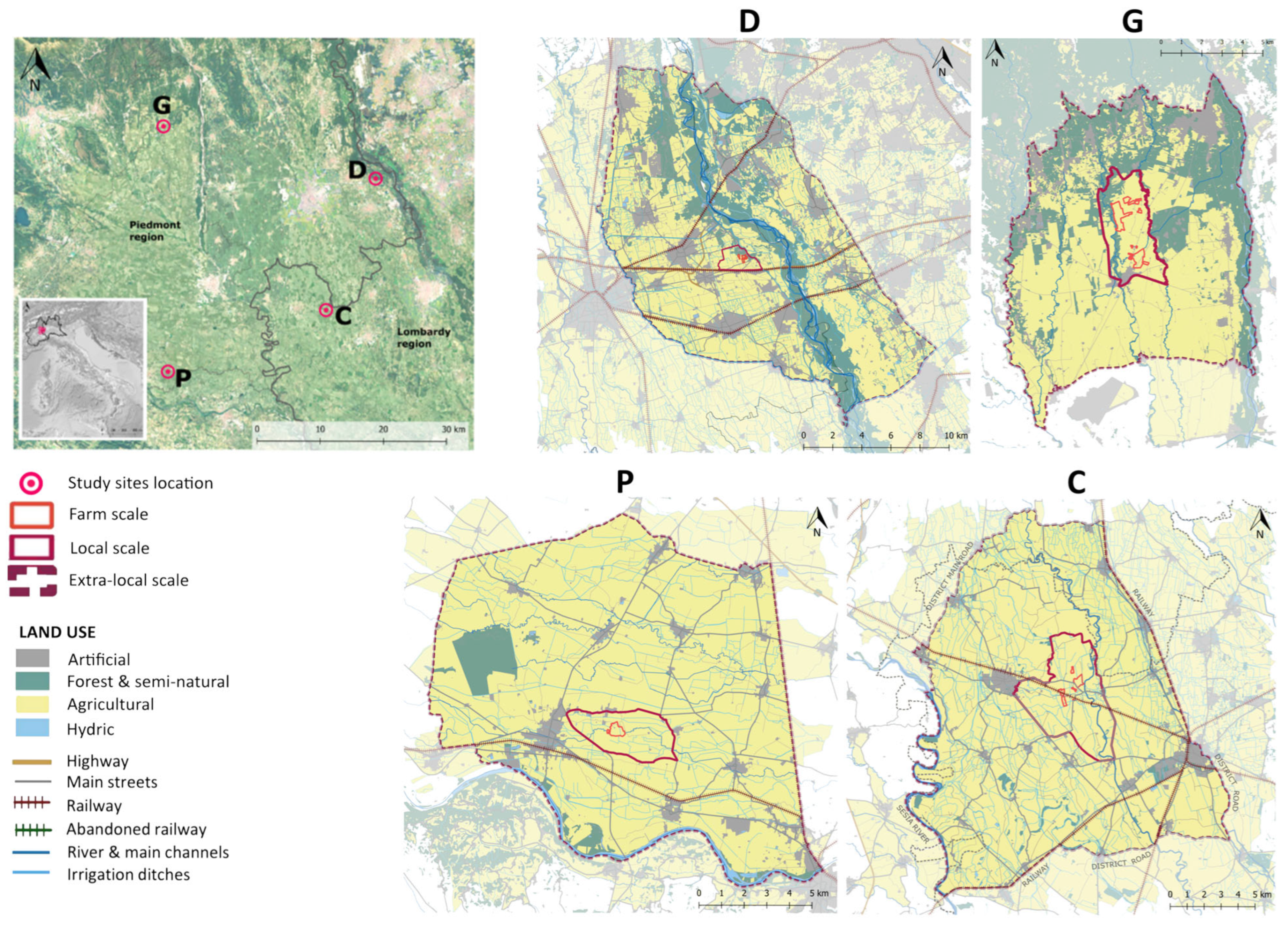
2.1. Case Studies

Analyses were conducted in four sites belonging to the western Po Plain (C, G, D, and P) (Figure 1), an alluvial district characterized by intensive land use traits with predominant conventional agricultural management (corn and soybean feeding livestock systems and rice), coupled with a widespread network of industrial districts, gray infrastructures, and urban centers. Po Plain agricultural landscapes suffer from high landscape oversimplification levels [23,24,42,44]. In such a context, green and blue infrastructure preservation and agroforestry-based management of agricultural systems can represent key strategies to counterbalance the impacts derived from land use intensification [40,41,42,44,85]. Nonetheless, their implementation is still lacking; only a few isolated farm experiences can be detected that implement an agroforestry, landscape-based farm management approach. The four sites chosen for this study include four agroforestry-based and biodiversity-oriented farms (farm scale—Fa), with each representing a unicum in the local agricultural landscape to which they belong. The studied farms (POLY farms) belong to the Polyculturae association, a non-profit organization supporting farmers’ efforts towards agrobiodiversity promotion; their farm management model is distinguished by crop diversification through rotations and cultivar use and preservation, minimum-to-zero chemical inputs, minimum soil disturbance and polyphyte cover cropping, in-field and between-fields agroforestry, and areal and linear landscape feature preservation and active management.

In each site, a farm scale and two landscape scales of analysis (extra-local (E_La) and local (La) scales) were identified (Figure 1). Landscape-scale analytical units’ boundaries were identified according to the landscape unit and ecotope concepts [86,87,88].

Their surrounding landscape system is generally dominated by conventional agricultural land uses, with some differences in the natural component preservation (G and D landscape systems show better green and blue infrastructure preservation compared to C and P sites).

Table 1. The main geomorphological and pedological [89,90], climatic [91,92], bioclimatic [49,93,94], and vegetational [95,96] traits of the study sites (D, G, P, and C).

		D	G	P	C
PEDOLOGY	ST/WRB CLASSES	Inceptisols	Alfisols (ancient terraces), inceptisols	Inceptisols, entisols	Luvisols, arenosols
	Geomorphology	Fluvial terrace	Riss alluvial terrace	Fluvial deposits	Fluvial terrace
	Main soil texture	Loamy skeletal	Fine silty	Loamy coarse, loamy sand	Loamy sand, sandy loam
	Development	Low pedogenesis	Intense pedogenesis	Low pedogenesis	Medium pedogenesis
	Permeability	High permeability	Surface hydromorphy	Medium permeability	Medium–low permeability
	pH	Acid to sub-acid	Acid	Sub-alkaline to alkaline	Sub-acid
	Land use capacity	III (stoniness)	III (oxygen availability)	II (oxygen availability)	IIw (waterlog)
	Specific traits	Dark epipedon
CLIMATE [1990–2022 data]	Annual rainfall [mm]	973	872	737	668
	Annual mean temperature [°C]	11.8	12.3	13.2	13.1
	Average maximum temperature [°C]	17.9	18.9	18.8	18.6
	Average minimum temperature [°C]	6.4	7.0	8.5	8.19
BIOCLIMATE [1990–2022 data]	Bioclimate (variant)	Temperate continental	Temperate continental (steppic)	Temperate continental (steppic)	Temperate oceanic (sub-Mediterranean)
	Bioclimatic belt	Upper mesotemperate Low humid	Upper mesotemperate Upper subhumid	Upper mesotemperate Low subhumid	Upper mesotemperate Low humid
VEGETATION	Climactic series	Western neutral-acidophilous Po Plain series of lower plain oak–hornbeam forests (Carpinion betuli Isler 1931 alliance)	Mosaic between western neutral-acidophilous Po Plain series of upper plain oak–hornbeam forests (Carpinion betuli Isler 1931 alliance), Central–Western pre-alpine acidophilous series of sessile oak forests (Quercion roboris Malcuit 1929 alliance, Phyteumato betonicifolium—Querco petraea sigmetum)	Western neutral-acidophilous Po Plain series of lower plain oak–hornbeam forests (Carpinion betuli Isler 1931 alliance)	Western neutral-acidophilous Po Plain series of lower plain oak–hornbeam forests (Carpinion betuli Isler 1931 alliance)

synthesizes the main geomorphological, pedological, climatic, bioclimatic, and vegetational traits of the sites studied.

2.2. Floristic and Vegetational Analyses

Field data were collected from the four study farms through floristic and phytosociological surveys in different habitats, which were chosen because of their representativeness of farm phytocoenosis-type composition. The monitored habitats included crop fields, crop field margins, rice fields, rice field margins, rice field interior embankments, wetlands, ditches, ditch banks, other margins, grasslands, orchards, hedgerows, and woods. Flora and vegetation surveys were carried out during the 2017–2023 growing seasons [97,98]. The analyzed database covered 7-year data, with the time span varying from site to site depending on their progressive involvement in the monitoring activities.

For each of the four sites, a floristic list was built on a farm scale. According to the national databases [99,100,101,102], each taxon was linked to the Raunkiær life forms (helophytes: He/I; therophytes: T; geophytes: G; hemicryptophytes: H; chamaephytes: C; and phanerophytes: P) [103], chorotypes and macro-chorotypes (6 biogeographical autochthonous regions: Eurasiatic, Mediterranean sensu latu (s.l.), Atlantic, boreal, wide distribution, and adventitious) [101], exotism classification (invasive archaeophyte, naturalized archaeophyte, cryptogenic, native, invasive neophyte, and naturalized neophyte) [99], and the related phytosociological class and maturity coefficient according to Taffetani’s method [66,67,104]. Scientific nomenclature refers to the Italian flora [99,100,101,102].

The study on vegetation integrated floristic analyses for sites where phytosociological relevés requirements were satisfied. Data collection and analysis were based on the phytosociological method [60,62,105,106,107]. Cover-abundance phytosociological indices (alpha-numerical Braun–Blanquet original scale) were transformed into corresponding percentage cover values, i.e., their central value according to Braun–Blanquet [60,108] and Tuxen–Ellenberg transformation [109]. Central values were used to compute the specific coverage index (SCI) [106,108]. The SCI allows for the performance of a species inside a plant community to be accounted for by better reflecting the phytosociological unit traits and overcoming the limits of a single survey in representing the real community traits [60,106,108]. The cover-weighted data enabled the calculation of α-diversity and maturity indices considering species presence and equal repartition.

The maturity index (IM) was computed on SCI data according to the Taffetani et al. method [66,67,104]. Each species is associated with a syntaxonomic class when it represents a diagnostic species for that class or for an alliance belonging to that class. Species attribution to syntaxonomic classes was based on the Italian vegetational prodrome data and literature comparison [66,67,95,96,104,110,111,112,113]. For species not representing diagnostic value, no class was attributed. Consequently, the maturity coefficient (m) or the edaphic coefficient (s) was attributed to each species according to Taffetani’s methodology [67].

Based on this information, we calculated a selection of indicators representing floristic–vegetational diversity, ecological, chorological, and maturity traits, which we considered relevant to an agricultural context (representation of biodiversity-related traits, floristic contamination degree, and anthropic disturbance-related traits).

Table 2. List of the applied farm-scale floristic and vegetational indicators.

	Category	Indicator	Abbreviation	Equation	Reference
FLORA	Richness	Species richness	SP_RICH	$\mathrm{S}\mathrm{P}\_\mathrm{R}\mathrm{I}\mathrm{C}\mathrm{H}={\displaystyle \sum _{\mathrm{i}=1}^{\mathrm{S}}}{\mathrm{n}.\mathrm{o}\mathrm{f} \mathrm{s}\mathrm{p}\mathrm{e}\mathrm{c}\mathrm{i}\mathrm{e}\mathrm{s}}_{\mathrm{i}}$
	Biological forms	He/I	He/I	$\mathrm{H}\mathrm{e}/\mathrm{I}={\displaystyle \frac{\sum _{\mathrm{i}=1}^{\mathrm{S}}{\mathrm{n}.\mathrm{o}\mathrm{f} \mathrm{H}\mathrm{e}/\mathrm{I} \mathrm{s}\mathrm{p}\mathrm{e}\mathrm{c}\mathrm{i}\mathrm{e}\mathrm{s}}_{\mathrm{i}}}{\sum _{\mathrm{i}=1}^{\mathrm{S}}{\mathrm{n}.\mathrm{o}\mathrm{f} \mathrm{s}\mathrm{p}\mathrm{e}\mathrm{c}\mathrm{i}\mathrm{e}\mathrm{s}}_{\mathrm{i}}}}$	[103]
		T	T	$\mathrm{T}={\displaystyle \frac{\sum _{\mathrm{i}=1}^{\mathrm{S}}{\mathrm{n}.\mathrm{o}\mathrm{f} \mathrm{T} \mathrm{s}\mathrm{p}\mathrm{e}\mathrm{c}\mathrm{i}\mathrm{e}\mathrm{s}}_{\mathrm{i}}}{\sum _{\mathrm{i}=1}^{\mathrm{S}}{\mathrm{n}.\mathrm{o}\mathrm{f} \mathrm{s}\mathrm{p}\mathrm{e}\mathrm{c}\mathrm{i}\mathrm{e}\mathrm{s}}_{\mathrm{i}}}}$	[103]
		G	G	$\mathrm{G}={\displaystyle \frac{\sum _{\mathrm{i}=1}^{\mathrm{S}}{\mathrm{n}.\mathrm{o}\mathrm{f} \mathrm{G} \mathrm{s}\mathrm{p}\mathrm{e}\mathrm{c}\mathrm{i}\mathrm{e}\mathrm{s}}_{\mathrm{i}}}{\sum _{\mathrm{i}=1}^{\mathrm{S}}{\mathrm{n}.\mathrm{o}\mathrm{f} \mathrm{s}\mathrm{p}\mathrm{e}\mathrm{c}\mathrm{i}\mathrm{e}\mathrm{s}}_{\mathrm{i}}}}$	[103]
		H	H	$\mathrm{H}={\displaystyle \frac{\sum _{\mathrm{i}=1}^{\mathrm{S}}{\mathrm{n}.\mathrm{o}\mathrm{f} \mathrm{H} \mathrm{s}\mathrm{p}\mathrm{e}\mathrm{c}\mathrm{i}\mathrm{e}\mathrm{s}}_{\mathrm{i}}}{\sum _{\mathrm{i}=1}^{\mathrm{S}}{\mathrm{n}.\mathrm{o}\mathrm{f} \mathrm{s}\mathrm{p}\mathrm{e}\mathrm{c}\mathrm{i}\mathrm{e}\mathrm{s}}_{\mathrm{i}}}}$	[103]
		C	C	$\mathrm{C}={\displaystyle \frac{\sum _{\mathrm{i}=1}^{\mathrm{S}}{\mathrm{n}.\mathrm{o}\mathrm{f} \mathrm{C} \mathrm{s}\mathrm{p}\mathrm{e}\mathrm{c}\mathrm{i}\mathrm{e}\mathrm{s}}_{\mathrm{i}}}{\sum _{\mathrm{i}=1}^{\mathrm{S}}{\mathrm{n}.\mathrm{o}\mathrm{f} \mathrm{s}\mathrm{p}\mathrm{e}\mathrm{c}\mathrm{i}\mathrm{e}\mathrm{s}}_{\mathrm{i}}}}$	[103]
		P	P	$\mathrm{P}={\displaystyle \frac{\sum _{\mathrm{i}=1}^{\mathrm{S}}{\mathrm{n}.\mathrm{o}\mathrm{f} \mathrm{P} \mathrm{s}\mathrm{p}\mathrm{e}\mathrm{c}\mathrm{i}\mathrm{e}\mathrm{s}}_{\mathrm{i}}}{\sum _{\mathrm{i}=1}^{\mathrm{S}}{\mathrm{n}.\mathrm{o}\mathrm{f} \mathrm{s}\mathrm{p}\mathrm{e}\mathrm{c}\mathrm{i}\mathrm{e}\mathrm{s}}_{\mathrm{i}}}}$	[103]
	Chorotypes	Adventitious	ADV	$\mathrm{A}\mathrm{D}\mathrm{V}={\displaystyle \frac{\sum _{\mathrm{i}=1}^{\mathrm{S}}{\mathrm{n}.\mathrm{o}\mathrm{f} \mathrm{A}\mathrm{D}\mathrm{V} \mathrm{s}\mathrm{p}\mathrm{e}\mathrm{c}\mathrm{i}\mathrm{e}\mathrm{s}}_{\mathrm{i}}}{\sum _{\mathrm{i}=1}^{\mathrm{S}}{\mathrm{n}.\mathrm{o}\mathrm{f} \mathrm{s}\mathrm{p}\mathrm{e}\mathrm{c}\mathrm{i}\mathrm{e}\mathrm{s}}_{\mathrm{i}}}}$
		Eurasiatic	EUR	$\mathrm{E}\mathrm{U}\mathrm{R}={\displaystyle \frac{\sum _{\mathrm{i}=1}^{\mathrm{S}}{\mathrm{n}.\mathrm{o}\mathrm{f} \mathrm{E}\mathrm{U}\mathrm{R} \mathrm{s}\mathrm{p}\mathrm{e}\mathrm{c}\mathrm{i}\mathrm{e}\mathrm{s}}_{\mathrm{i}}}{\sum _{\mathrm{i}=1}^{\mathrm{S}}{\mathrm{n}.\mathrm{o}\mathrm{f} \mathrm{s}\mathrm{p}\mathrm{e}\mathrm{c}\mathrm{i}\mathrm{e}\mathrm{s}}_{\mathrm{i}}}}$
		Wide distr.	WIDE	$\mathrm{W}\mathrm{I}\mathrm{D}\mathrm{E}={\displaystyle \frac{\sum _{\mathrm{i}=1}^{\mathrm{S}}{\mathrm{n}.\mathrm{o}\mathrm{f} \mathrm{W}\mathrm{I}\mathrm{D}\mathrm{E} \mathrm{s}\mathrm{p}\mathrm{e}\mathrm{c}\mathrm{i}\mathrm{e}\mathrm{s}}_{\mathrm{i}}}{\sum _{\mathrm{i}=1}^{\mathrm{S}}{\mathrm{n}.\mathrm{o}\mathrm{f} \mathrm{s}\mathrm{p}\mathrm{e}\mathrm{c}\mathrm{i}\mathrm{e}\mathrm{s}}_{\mathrm{i}}}}$
	Allochthony	Alien/total species	ALIEN	$\mathrm{A}\mathrm{L}\mathrm{I}\mathrm{E}\mathrm{N}={\displaystyle \frac{\sum _{\mathrm{i}=1}^{\mathrm{S}}{\mathrm{n}.\mathrm{o}\mathrm{f} \mathrm{A}\mathrm{L}\mathrm{I}\mathrm{E}\mathrm{N} \mathrm{s}\mathrm{p}\mathrm{e}\mathrm{c}\mathrm{i}\mathrm{e}\mathrm{s}}_{\mathrm{i}}}{\sum _{\mathrm{i}=1}^{\mathrm{S}}{\mathrm{n}.\mathrm{o}\mathrm{f} \mathrm{s}\mathrm{p}\mathrm{e}\mathrm{c}\mathrm{i}\mathrm{e}\mathrm{s}}_{\mathrm{i}}}}$
		Invasive alien/alien	INVAS	$\mathrm{I}\mathrm{N}\mathrm{V}\mathrm{A}\mathrm{S}={\displaystyle \frac{\sum _{\mathrm{i}=1}^{\mathrm{S}}{\mathrm{n}.\mathrm{o}\mathrm{f} \mathrm{I}\mathrm{N}\mathrm{V}\mathrm{A}\mathrm{S} \mathrm{s}\mathrm{p}\mathrm{e}\mathrm{c}\mathrm{i}\mathrm{e}\mathrm{s}}_{\mathrm{i}}}{\sum _{\mathrm{i}=1}^{\mathrm{S}}{\mathrm{n}.\mathrm{o}\mathrm{f} \mathrm{s}\mathrm{p}\mathrm{e}\mathrm{c}\mathrm{i}\mathrm{e}\mathrm{s}}_{\mathrm{i}}}}$
VEGETATION	Diversity	Shannon equitability index	H’/H’max	${\displaystyle \frac{{\mathrm{H}}^{\prime }}{\mathrm{H}\mathrm{m}\mathrm{a}\mathrm{x}}}={\displaystyle \frac{{\mathrm{H}}^{\prime }}{\ln \left(\mathrm{S}\right)}}$ with ${\mathrm{H}}^{\prime }=-{\displaystyle \sum _{\mathrm{i}=1}^{\mathrm{S}}}{\mathrm{p}}_{\mathrm{i}}\times \mathrm{l}\mathrm{n}{\mathrm{p}}_{\mathrm{i}}$	[114]
		Naturalness index	N	$\mathrm{N}={\displaystyle \frac{{\mathrm{H}}_{\mathrm{a}\mathrm{u}\mathrm{t}\mathrm{o}\mathrm{c}\mathrm{h}}^{\prime }}{{\mathrm{H}}^{\prime }}}$ with ${\mathrm{H}}^{\prime }\_\mathrm{a}\mathrm{u}\mathrm{t}\mathrm{o}\mathrm{c}\mathrm{h}=-{\displaystyle \sum _{\mathrm{i}=1}^{\mathrm{S}}}{\mathrm{p}}_{\mathrm{i}\_\mathrm{a}\mathrm{u}\mathrm{t}\mathrm{o}\mathrm{c}\mathrm{h}}\times \mathrm{l}\mathrm{n}{\mathrm{p}}_{\mathrm{i}\_\mathrm{a}\mathrm{u}\mathrm{t}\mathrm{o}\mathrm{c}\mathrm{h}}$	[115]
		Gini–Simpson diversity index	1-lambda	$1-\lambda =1-\left({\displaystyle \sum _{\mathrm{i}=1}^{\mathrm{R}}}{{\mathrm{p}}_{\mathrm{i}}}^2\right)$	[116]
	Maturity	Index of maturity	IM	$\mathrm{I}\mathrm{M}={\displaystyle \frac{\sum _{\mathrm{j}=1}^{\mathrm{n}}{\mathrm{S}\mathrm{C}\mathrm{I}}_{\mathrm{i}}\times (\mathrm{m},\mathrm{s})}{{\mathrm{S}\mathrm{C}\mathrm{I}}_{\mathrm{t}\mathrm{o}\mathrm{t}}}}$	[66,67,104]

reports the floristic and vegetational indicators, which were selected for comparative analysis.

2.3. Landscape Ecology Analyses

Landscape ecology analyses were led in each of the four sites at extra-local (E_La) and local (La) scales. E_La and La landscape analytical unit boundaries were identified according to the landscape unit and ecotope concepts [86,87,88]. According to a multi-scale analytical methodology already tested on the study sites [40,41,42,43,44], different degrees of analytical detail were set for E_La and La scales.

For extra-local-scale analyses, the single-patch land-use-type categorization was based on land cover maps [90], which were validated through satellite images in doubtful cases [117]. For local scale, patch boundaries were based on satellite images, regional land cover maps, and quick field checks. For both the E_La and La scales, patch surfaces and perimeters were cumulated for each land use category, which were clustered in three main landscape subsystems [forest and seminatural (NAT), agricultural (AGR), and artificial (ART)] according to Corine Land Cover classification [118].

According to the results of the multi-scale analytical methodology test in the sites studied [40,42,44], a set of landscape ecology indicators was chosen for each scale of analysis, representing the most informative and least redundant indicator set for the studied agricultural context.

Table 3. List of the applied extra-local (E_La) and local (La) scale landscape ecology indicators. TOT: total landscape system; NAT: forest and semi-natural landscape subsystem; AGR: agricultural landscape subsystem.

	Indicator	Scale	Equation	References
Basic structural traits	Matrix (MTX) x = [NAT; AGR]	E_La La	${\mathrm{M}\mathrm{T}\mathrm{X}}_{\mathrm{x}}={\displaystyle \frac{\sum _{\mathrm{i}=1}^{\mathrm{n}}{\mathrm{A}}_{\mathrm{i}\mathrm{x}}\times 100}{{\mathrm{A}}_{\mathrm{t}\mathrm{o}\mathrm{t}}}}$ Ai = total area of each land use categories patch Atot = total area	[32]
Diversity indices	Diversity (DIV) X = [DIV_TOT; DIV_NAT; DIV_AGR]	E_La La	${\mathrm{D}\mathrm{I}\mathrm{V}}_{\mathrm{x}}=-{\sum }_{\mathrm{i}=1}^{\mathrm{n}}{\displaystyle \frac{{\mathrm{A}}_{\mathrm{i}}}{{\mathrm{A}}_{\mathrm{t}\mathrm{o}\mathrm{t}}}}\times \mathrm{l}\mathrm{n}{\displaystyle \frac{{\mathrm{A}}_{\mathrm{i}}}{{\mathrm{A}}_{\mathrm{t}\mathrm{o}\mathrm{t}}}}$	[32]
Connectivity indices	Connectivity (CON)	La	$\mathrm{C}\mathrm{O}\mathrm{N}={\displaystyle \frac{\mathrm{L}}{[3\times \left(\mathrm{N}-2\right)]}}$ L = no. of links N = no. of nodes	[119]
	Weighted connectivity (WCON)	La	$\mathrm{W}\mathrm{C}\mathrm{O}\mathrm{N}={\displaystyle \frac{{\sum }_{\mathrm{i}=1}^5{\mathrm{L}}_{\mathrm{i}}\times {\mathrm{W}}_{\mathrm{i}}}{[3\times \left(\mathrm{N}-2\right)]}}$  Li = no. of links for each Ecological Quality Class (EQCi = [1,2,3,4,5]) Wi = EQCi weight: ${\mathrm{W}}_{\mathrm{i}}={\displaystyle \frac{{\mathrm{E}\mathrm{Q}\mathrm{C}}_{\mathrm{i}}}{{\mathrm{E}\mathrm{Q}\mathrm{C}}_{\mathrm{m}\mathrm{a}\mathrm{x}}}}$	[41]
	Circuitry (CIR)	La	$\mathrm{C}\mathrm{I}\mathrm{R}={\displaystyle \frac{(\mathrm{L}-\mathrm{N}+1)}{[2\times \left(\mathrm{N}-5\right)]}}$	[119]
	Weighted circuitry (WCIR)	La	$\mathrm{W}\mathrm{C}\mathrm{I}\mathrm{R}={\displaystyle \frac{\left[\right({\sum }_{\mathrm{i}=1}^5{\mathrm{L}}_{\mathrm{i}}\times {\mathrm{W}}_{\mathrm{i}})-\mathrm{N}+1)]}{[2\times \left(\mathrm{N}-5\right)]}}$ Li = no. of links for each Ecological Quality Class (EQCi = [1,2,3,4,5]) Wi = EQCi weight (as above)	[41]
Indices on ecological functionality	Mean biological territorial capacity (MBTC) X = [MBTC_TOT; MBTC _NAT; MBTC_AGR]	E_La La (only MBTC_TOT)	$\mathrm{M}\mathrm{B}\mathrm{T}\mathrm{C}={\displaystyle \frac{{\sum }_{\mathrm{i}=1}^{\mathrm{m}}{\mathrm{B}\mathrm{T}\mathrm{C}}_{\mathrm{i}}\times {\mathrm{A}}_{\mathrm{i}}}{{\mathrm{A}}_{\mathrm{t}\mathrm{o}\mathrm{t}}}}$	[88,120,121]

reports the selected E_La and La landscape ecology indicators.

2.4. Inter-Scale Comparisons of Landscape Ecology and Floristic–Vegetational Traits

The floristic and vegetational indicator values computed at the farm scale were gathered for the four POLY farms. Parallelly, the extra-local-scale and local-scale landscape ecology index values were gathered for the four POLY farms.

A Shapiro–Wilk normality test was run on the selected floristic, vegetational, and landscape ecology indicators. Consequently, a correlation test was run (linear r Pearson correlation coefficient test) between the floristic–vegetational indicators, followed by between the floristic–vegetational indicators and the landscape ecology ones (for each separate scale of analysis).

2.5. Mapping Inter-Scale Biodiversity

The local-scale mapping of biodiversity as a life support ecosystem service was based on Burckhard’s land-use-based ES assessment methodology [82,122]. The applied ES matrix followed the Burkhard’s matrix readaptation for Po Plain agricultural landscapes peculiarities [42], which provided a more accurate representation of Po Plain typical land use types by integrating the life support ES evaluation according to European and/or global meta-analyses and local studies and correcting the ES delivering values according to the biological territorial capacity (BTC) values of each land use [86,88,120]. Specifically, the habitat and biodiversity ES was evaluated [7,123].

According to previous studies ([42,124]), for each land use type, we considered the percentage ratio between the current value of the habitat and biodiversity ES and the maximum theoretical value to obtain normalized values ranging from 0 to 100 and transfer the results into a spatial representation.

The obtained ES map represented the contribution of each patch of the local landscape under assessment to biodiversity.

The local-scale mapping of landscape diversity was based on the spatial representation of each patch’s contribution to total landscape diversity based on the landscape diversity value (see Table 3) of the landscape subsystem it belongs to (NAT, AGR, and ART). The landscape diversity index (DIV) was used in its normalized version to enable its comparison, as follows:

$${\mathrm{D}\mathrm{I}\mathrm{V}2}_{\mathrm{x}}={\displaystyle \frac{-{\sum }_{\mathrm{i}=1}^{\mathrm{n}}\frac{{\mathrm{A}}_{\mathrm{i}}}{{\mathrm{A}}_{\mathrm{t}\mathrm{o}\mathrm{t}}}\times \mathrm{l}\mathrm{n}\frac{{\mathrm{A}}_{\mathrm{i}}}{{\mathrm{A}}_{\mathrm{t}\mathrm{o}\mathrm{t}}}}{\mathrm{l}\mathrm{n}\mathrm{S}}}$$

where x = each landscape subsystem (TOT, NAT, AGR, and ART), A_i = total area of each land use category patches, A_tot = total area, S = number of land use categories, and lnS = maximum DIV_x value (*cit.).

Inter-scale biodiversity maps were built by matching two pieces of complementary information, i.e., by representing, for each patch, the arithmetic product between DIV2_TOT and habitat and biodiversity ES (both ranging from 0 to 100). This resulted in maps that represented inter-scale biodiversity patterns, i.e., each single patch of habitat and biodiversity ES provisioning capacity weighted on local landscape diversity values. This inter-scale operation was based on the detected inter-scale relationships between landscape diversity values and farm-scale species richness and α-diversity values, which were also confirmed by scientific literature [17,34,46,69,74,75,79,125,126,127].

3. Results

3.1. Dataset Exploration

Appendix A reports the results of the farm-scale floristic and vegetational indicators (

Table A1. Results of the farm-scale floristic and vegetational indicators for each study site (D, G, P, and C).

Category		Index	U.o.M.	D	G	P	C
FLORA	Richness	SP_RICH	n.	129	225	70	156
	Biological forms	He/I	%	0.5	0.2	0.14	5
		T	%	0.25	0.18	0.26	0.25
		G	%	0.13	0.9	0.11	0.14
		H	%	0.39	0.44	0.41	0.35
		C	%	0.3	0.4	0.3	0.1
		P	%	0.15	0.23	0.4	0.21
	Chorotypes	ADV	%	0.22	0.16	0.24	0.18
		EUR	%	0.29	0.36	0.14	0.27
		WIDE	%	0.33	0.27	0.40	0.31
	Allochthony	ALIEN	%	0.27	0.20	0.28	0.24
		INVAS	%	0.74	0.55	0.63	0.59
VEGETATION	Diversity	H’/H’max	-	0.51	0.58	0.5	0.57
		N	-	0.91	0.88	0.96	0.94
		1-lambda	-	0.85	0.82	0.67	0.82
	Maturity	IM	-	3	1.1	0.7	0.6

) and the extra-local-scale and local-scale landscape ecology indicators computed on each study site (

Table A2. Results of the extra-local-scale and local-scale landscape ecology indicators computed on each study site (D, G, P, and C).

			Extra-Local				Local
	Index	U.o.M.	D	G	P	C	D	G	P	C
Matrix	AGR	%	0.55	0.60	0.87	88.56	0.70	0.69	0.93	0.93
	NAT	%	0.27	0.31	0.06	0.05	0.24	0.26	0.04	0.04
Diversity	DIV_TOT	-	2.13	1.7	1.11	1.09	1.55	1.81	0.74	0.79
	DIV_NAT	-	0.59	0.51	0.25	0.23	0.48	0.59	0.21	0.22
	DIV_AGR	-	0.92	0.8	0.56	0.6	0.84	1.03	0.42	0.45
Biological territorial capacity	MBTC_TOT	Mcal/ha/yr	1.88	2.39	1.26	1.17	2.22	2.56	1.16	1.18
	MBTC_NAT	Mcal/ha/yr	4.51	5.32	3.48	2.52
	MBTC_AGR	Mcal/ha/yr	1.01	1.14	1.14	1.14
Connectivity & circuitry	CON	-					0.33	0.39	0.36	0.24
	WCON	-					0.22	0.3	0.16	0.12
	CIR	-					−0.01	0.08	0.03	−0.14
	WCIR	-					−0.18	−0.05	−0.28	−0.32

). Almost all farm-scale floristic and vegetational data are normally distributed (

Table 4. (A) Shapiro–Wilk normality test results of the farm-scale floristic and vegetational indicators—species richness: SP_RICH; Shannon equitability index: H’/H’max; naturalness index: N; Gini–Simpson diversity index: 1-λ’; therophytes: T; hemicryptophytes: H; chamaephytes: C; phanerophytes: P; adventitious macro-chorotype: ADV; Eurasiatic macro-chorotype: EUR; wide distribution macro-chorotype: WIDE; alien species ratio: ALIEN; invasiveness degree: INVAS; and index of maturity: IM. (B) Shapiro–Wilk normality test results of the extra-local-scale (E_La) and local-scale (La) landscape ecology indices—agricultural components ratio: AGR; natural components ratio: NAT; landscape total diversity: DIV_TOT; diversity of the agricultural components: DIV_AGR; diversity of the natural and semi-natural components: DIV_NAT; extra-local total mean biological territorial capacity: MBTC_TOT; extra-local mean biological territorial capacity of the agricultural components: MBTC_AGR; and extra-local mean biological territorial capacity of the natural and semi-natural components: MBTC_NAT. Bold values: normally distributed data.

(A)	FLORISTIC–VEGETATIONAL INDICES
	Farm scale
	SP_RICH	H’/H’max	N	1-lambda	He/I.	T.	G.	H.	C.	P.	ADV	EUR	WIDE	ALIEN	INVAS	IM
N	4	4	4	4	4	4	4	4	4	4	4	4	4	4	4	4
Shapiro–Wilk W	0.99	0.84	0.98	0.77	0.80	0.73	0.92	0.98	0.91	0.90	0.97	0.93	0.96	0.87	0.95	0.77
p(normal)	0.98	0.21	0.89	0.06	0.10	0.03	0.52	0.88	0.47	0.42	0.83	0.59	0.80	0.30	0.73	0.06
	LANDSCAPE ECOLOGY INDICES
(B)	Extra-local scale								Local scale
	AGR	NAT	DIV_TOT	DIV_AGR	DIV_NAT	MBTC_TOT	MBTC_AGR	MBTC_NAT	AGR	NAT	DIV_TOT	DIV_NAT	DIV_AGR	MBTC_TOT	CON	WCON	CIR	WCIR
N	4	4	4	4	4	4	4	4	4	4	4	4	4	4	4	4	4	4
Shapiro–Wilk W	0.82	0.82	0.87	0.91	0.85	0.90	0.65	0.99	0.75	0.79	0.85	0.86	0.87	0.84	0.92	0.96	0.94	0.95
p(normal)	0.15	0.13	0.31	0.49	0.22	0.45	0.002	0.93	0.04	0.08	0.23	0.25	0.29	0.19	0.55	0.78	0.64	0.71

(A)), except for therophyte values (T), whose values are close to a normal distribution (p normal = 0.03). Similarly, almost all extra-local and local landscape ecology data (La) are normally distributed (Table 4(B)), except for the extra-local landscape agricultural components ratio (AGR), whose values are not normally distributed (p normal = 0.002), and the local landscape agricultural components ratio (AGR), whose values are close to a normal distribution (p normal = 0.04). Data transformation failed to obtain normally distributed data. Because of the predominance of normally distributed data, the Pearson r correlation analysis was chosen for this dataset.

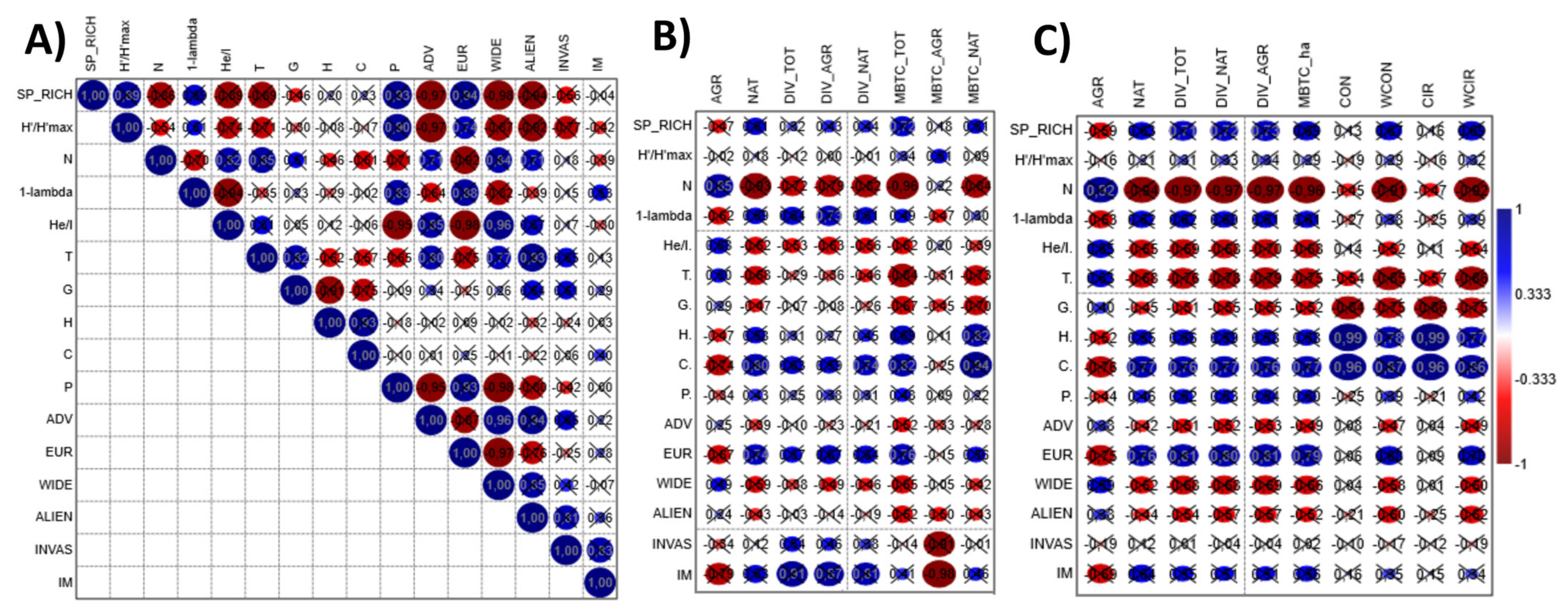
3.2. Floristic–Vegetational Indicator Correlation Patterns

Most correlation indices (Figure 2A) are not significant from a statistical point of view due to the limited sample size (four values, representing each farm value). Nonetheless, the highlighted patterns show some interesting behaviors, which can be summarized as follows:

Species richness (SP_RICH) shows high positive correlation coefficient values with the Shannon equitability index (H’/H’max) and the Gini–Simpson diversity index (1-λ’).

SP_RICH is also positively correlated with the phanerophyte ratio over total farm flora (P) and Eurasiatic species presence (EUR).

In contrast, SP_RICH is negatively correlated to the naturalness index (N), therophyte ratio (T), adventitious (ADV), wide distribution (WIDE), alien (ALIEN), and invasive (INVAS) species.

The Shannon equitability index (H’/H’max) and the Gini–Simpson diversity index (1-λ’) show similar relationships with the other indices; the Gini–Simpson diversity index generally has lower correlation coefficient values with indicators representing floristic contamination (ADV, ALIEN, and INVAS) and therophytes (T).

The therophyte ratio (T) is negatively correlated with hemicryptophytes (H), chamaephytes (C), and phanerophyte ratio (P), as well as with the Eurasiatic species ratio (EUR).

In contrast, the therophyte ratio shows high positive correlation coefficient values with indicators representing floristic contamination (ADV, WIDE, ALIEN, and INVAS).

The phanerophyte ratio (P) shows an opposite behavior to therophytes: P shows a positive correlation coefficient value with Eurasiatic species (EUR), while it shows negative correlation coefficient values with indicators representing the floristic contamination (ADV, WIDE, ALIEN, and INVAS).

The index of maturity (IM) does not show any relevant correlation pattern with the other indicators.

3.3. Floristic–Vegetational and Extra-Local Landscape Ecology Indicators’ Correlation Patterns

Figure 2B reports the results of the linear Pearson correlation analysis run between the farm-scale floristic and vegetational indicators and the landscape ecology indices computed on each farm’s extra-local landscape.

Most correlation indices are not significant from a statistical point of view due to the limited sample size (four values, representing each farm value). Nonetheless, the highlighted patterns suggest some interesting behaviors, which can be summarized as follows:

Species richness (SP_RICH) values show positive correlation coefficient values with the extra-local landscape’s natural components ratio (NAT), the mean extra-local-scale biological territorial capacity values of the total landscape (MBTC_TOT), and the mean extra-local-scale biological territorial capacity values of the natural and semi-natural components (MBTC_NAT) and slight positive correlation values (0.32 ≤ r ≤ 0.44) with the extra-local landscape total diversity values (DIV_TOT) and the diversity of the local natural and agricultural components (DIV_NAT and DIV_AGR).

Higher agricultural components in the extra-local landscape (AGR) tend to be related to lower species richness (SP_RICH).

The Shannon equitability index does not show relevant correlation patterns with extra-local landscape ecological traits (the Pearson r correlation coefficient is always lower or close to 0.5).

The Gini–Simpson diversity index shows similar correlation patterns to the ones shown by the SP_RICH indicator, with higher r coefficient values for the landscape diversity indicators (>0.5); the positive relationship with total mean biological territorial capacity slightly decreases compared to SP_RICH (0.49).

Higher agricultural components in the extra-local landscape (AGR) tend to be related to lower Gini–Simpson diversity values.

The naturalness index shows an opposite relationship with the extra-local landscape matrix, diversity, and mean biological territorial capacity traits. This reflects the anomalous behavior of this index, as already highlighted in farm-scale analyses, due to the intense floristic and vegetational contamination by alien taxa.

The presence of therophytes (T) is positively correlated with the extra-local landscape agricultural components ratio (AGR), whereas it is negatively correlated with the local landscape’s natural components ratio (NAT), the total mean biological territorial capacity (MBTC_TOT), and the total mean biological territorial capacity of natural and semi-natural components (MBTC_NAT). Also, the extra-local diversity values (DIV_TOT, DIV_NAT, and DIV_AGR) show negative relationships with T, but Pearson correlation values are low (−0.46 ≤ r ≤ −0.29).

Geophytes (G) show a similar behavior to T, with more relevant relationships (higher Pearson coefficient values) for MBTC_TOT (−0.67) and MBTC_NAT (−0.70).

Hemicryptophytes (H), chamaephytes (C), and phanerophytes (P) show an opposite behavior: they are more present when the extra-local landscape has a lower agricultural components ratio (AGR) to the advantage of the natural components (NAT), higher extra-local landscape diversity, and total mean biological territorial capacity values (especially for H and C; p is <0.50).

Adventitious (ADV) and alien (ALIEN) species ratio indicators only show relevant negative correlation patterns with the extra-local total mean biological territorial capacity values (−0.52 and −0.62, respectively).

The wide distribution (WIDE) species ratio indicator shows more relevant positive correlation patterns with the extra-local agricultural components ratio (AGR), while they are negatively correlated to the other local landscape ecological indices related to natural component presence, diversification, and mean biological territorial capacity.

Eurasiatic species (EUR) show the opposite correlation patterns, with higher Pearson coefficient values (0.56 ≤ r ≤ 0.76).

The index of maturity (IM) shows a relationship with landscape ecology indices similar to the one of species richness; the Gini–Simpson diversity index; H, C, and P biological forms; and Eurasiatic species: it is positively correlated to the local landscape’s natural and semi-natural components’ presence (NAT), the diversity indices (relevant Pearson coefficient values, 0.81 ≤ r ≤ 0.91), and its mean biological territorial capacity, while it is negatively correlated to the extra-local landscape’s agricultural components ratio (the higher the agricultural components, the lower the POLY farm rice land wild phytocoenosis maturity degree).

3.4. Floristic–Vegetational and Local Landscape Ecology Indicator Correlation Patterns

Figure 2C reports the results of the linear Pearson correlation analysis run between the floristic and vegetational indicators and the landscape ecology indices computed on each farm’s local landscape.

Most correlation indices are not significant from a statistical point of view due to the limited sample size (four values, representing each farm value). Nonetheless, the highlighted patterns show some interesting behaviors, which can be summarized as follows:

Species richness (SP_RICH) values show positive correlation coefficient values with the local landscape’s natural components ratio (NAT), its total diversity values (DIV_TOT), the diversity of the local natural and agricultural components (DIV_NAT and DIV_AGR), the mean local-scale biological territorial capacity values (MBTC_ha), and the connectivity and circuitry values of their variants weighted on the links’ ecological quality classes (WCON and WCIR). The correlation values of all these indices are generally higher than for the extra-local scale.

As for the extra-local landscape, the agricultural components in the local landscape (AGR) also tend to be related to lower species richness (SP_RICH), with a higher Pearson coefficient value (−0.59).

As for the extra-local landscape, the Shannon equitability index does not show relevant correlation patterns with local landscape ecological traits (the Pearson r correlation coefficient is always lower than 0.5).

As for the extra-local landscape, the Gini–Simpson diversity index shows similar correlation patterns to the ones shown by the SP_RICH indicator, except for the correlation with WCON and WCIR values, which is lower than 0.5.

The naturalness index shows an opposite relationship with the extra-local landscape matrix, diversity, and mean biological territorial capacity traits compared to the floristic richness and vegetational diversity indicators. This reflects the anomalous behavior of this index, as already highlighted in farm-scale analyses, due to the intense floristic and vegetational contamination by alien taxa.

Similarly to the extra-local scale, the presence of therophytes (T) is positively correlated with the local landscape’s agricultural components ratio (AGR), whereas it is negatively correlated with the local landscape’s natural components ratio (NAT), its diversity values (DIV_TOT, DIV_NAT, and DIV_AGR), and its connectivity values (CON, WCON, CIR, and WCIR). The local landscape diversity values show a higher negative correlation pattern with T compared to the extra-local scale.

Geophytes (G) show a similar behavior to T.

Hemicryptophytes (H), chamaephytes (C), and phanerophytes (P) show an opposite behavior: like for extra-local landscape, they are more present when the local landscape has a lower agricultural components ratio (AGR) to the advantage of the natural components (NAT); they are positively correlated with local landscape diversity values (DIV_TOT, DIV_NAT, and DIV_AGR) and its connectivity values (CON, WCON, CIR, and WCIR). Correlation is high and significant (p < 0.05) between H and C with CON and CIR indices.

Similarly to extra-local scale, adventitious (ADV), wide distribution (WIDE), and alien (ALIEN) species ratio indicators are positively correlated to the agricultural components ratio (AGR), while they are negatively correlated to the other local landscape ecological indices related to natural component presence, diversification, connectivity, and circuitry.

Eurasiatic species (EUR) show the opposite correlation patterns.

The index of maturity (IM) shows a relationship with landscape ecology indices similar to the one of species richness; the naturalness index; the Gini–Simpson diversity index; H, C, and P biological forms; and Eurasiatic species: it is positively correlated to the local landscape diversity indices, its naturalness components ratio, its mean biological territorial capacity, and connectivity values, while it is negatively correlated to the local landscape agricultural components ratio (the higher the agricultural components, the lower the POLY farm rice land wild phytocoenosis maturity degree).

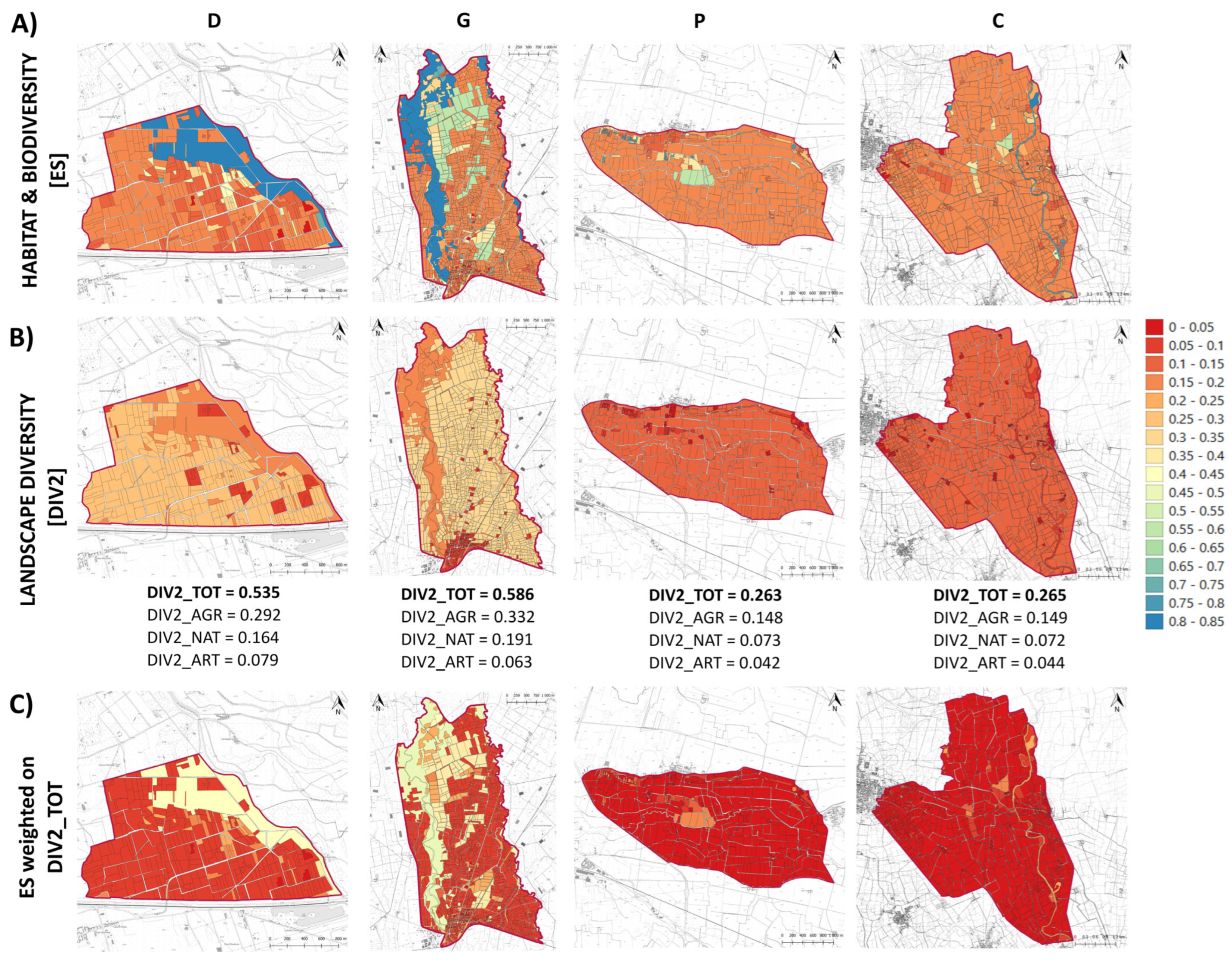
3.5. Inter-Scale Biodiversity Maps

Considering the dependence of farm-scale floristic richness and vegetational α-diversity values on local-scale landscape ecological status and, particularly, landscape diversity values, this section investigates the spatial relationships between local landscape diversity values and patch-scale biodiversity contributions, represented here through land-use-based support ecosystem services (habitat and biodiversity ES). Figure 3 represents, for each case study, the local-scale habitat and biodiversity ES maps, the landscape diversity maps, and the resulting inter-scale biodiversity maps (Figure 3).

These maps clearly distinguish the D-G sites from P-C ones, with the latter showing a clearly limited occurrence of patches with medium–high habitat and biodiversity ES values (Figure 3A) and a generalized low level of landscape diversity (Figure 3B). D-G sites show higher landscape diversification of the agricultural subsystem components, whereas P-C sites are highly simplified (Figure 3B). These traits result in a significant decrease in habitat and biodiversity ES delivering capacity of single P-C patches if weighted on landscape total diversity (DIV2_TOT) (Figure 3C). D-G sites register a decrease in habitat and biodiversity ES delivery capacity too, but their reduction is limited compared to P-C: ES delivery capacity is preserved for natural components and for agricultural components under Polyculturae management (crop diversification, no chemical use, minimum soil disturbance, agroforestry practices, and agrobiodiversity support measures) (Figure 3C).

4. Discussion

Species richness and α-diversity indices tend to follow similar patterns, with a similar positive relationship with Eurasiatic species, whereas they all tend to be negatively related to adventitious, wide distribution, and alien species ratios. In particular, higher statistical significance is reported for species richness and Shannon equitability negative correlation with adventitious species; species richness is significantly negatively correlated to wide distribution species ratio too. In our case, lower negative correlation values were found with invasive traits of alien species, suggesting a lower dependence of diversity values on invasive behaviors. These results are aligned with the widely reported negative influence of allochthonous species on floristic and phytocoenosis diversity values [128,129,130,131] and confirm the importance of proper management and design of interventions on rural landscape features to effectively sustain higher floristic and vegetational diversity values in agricultural land [132].

Data also suggest a role of disturbance conditions towards diversity values. First of all, the alien species ratio is generally positively related to anthropic disturbance and tends to be a consequence of it, as various previous studies have already outlined [133,134,135] and as confirmed by alien species distribution in habitat types and landscape types with different anthropic disturbance degrees [23,83,136]. Moreover, as shown in our study, species richness and α-diversity indices show positive correlation patterns with the phanerophyte ratio, whereas they tend to decrease when a higher therophyte species ratio occurs. Therophytes generally show a negative relationship with hemicryptophytes, chamaephytes, and phanerophyte species ratio. In agricultural contexts, therophyte presence is easily influenced by recurrent and/or severe anthropic disturbance conditions (frequent and intense soil disturbance, widespread herbicide application, etc.), which are typically associated with therophyte traits: small and numerous seeds, fast growth rate, and short generation time [58,59,68,137]. Specifically, short generation time plays a larger role when severe disturbance conditions occur [138]. In contrast, higher medium–long cycle species presence in rural contexts (hemicryptophytes, chamaephytes, and, especially, phanerophytes) is made possible by lower intensity and frequency of anthropic disturbance [58,139].

In turn, the phanerophyte ratio tends to increase with the Eurasiatic species ratio, while they are less represented when adventitious, wide distribution, and alien species ratios increase. In contrast, the therophyte species ratio increases with floristic contamination, confirming their positive relationship with phytocoenosis disturbance traits, as outlined in the literature [58,59,68,137].

These traits are consistent with the thesis that higher disturbance conditions tend to promote lower on-farm floristic and vegetational diversity and that the promotion of more stable conditions (i.e., allowing for phanerophyte species to develop) positively helps in counterbalancing the negative effects of floristic contamination on farm-scale α-diversity and, generally, farm-scale floristic and vegetational ecological quality.

This was not confirmed by the index of maturity values, which generally did not show relevant correlation patterns with other indicators.

The naturalness index showed contrasting behaviors (see Appendix A and Table A1), suggesting some applicability limits in highly alien-disturbed phytocoenoses, such as the ones in agricultural contexts. When the alien species ratio is high and their equal distribution is low, then the Shannon equitability index computed on the autochthonous species subset increases, raising the naturalness index values (higher than 1); despite the total number of species being lower (and hence lower Shannon equitability values are expected), species equal distribution significantly rises because of the exclusion of highly abundant alien species. In such cases, the naturalness index increase cannot be interpreted as a consequence of lower contamination by allochthonous species and does not express higher phytocoenosis naturalness values; on the contrary, it is a consequence of intense alien species competition. This bias derives from the application of a plant community-based indicator (Shannon equitability) on theoretical plant communities that do not correspond to real ones (a theoretical version of real phytocoenoses, excluding alien species); when applied to phytocoenoses dominated by alien species, such an approach brings misleading information. These interpretations are consistent with the positive correlation coefficient values that we found between naturalness and adventitious, wide distribution, and alien species and landscape agricultural components ratio and the negative correlation coefficient values when considering Eurasiatic species and landscape ecological quality parameters (natural components ratio, landscape diversity, MBTC, and connectivity). Such results are contrasting compared to the ones expected by previous applications of this index in Mediterranean phytocoenoses, which identified a range of 0–1 for the index [115]. This suggests the need for further testing of the naturalness index on wider datasets, also focusing on the relationship between the naturalness index and alien taxa presence and abundance in both Mediterranean and temperate phytocoenosis types belonging to different contexts (urban, agricultural, and natural).

Wet habitats (helophytes and hydrophyte species ratio) show higher floristic–vegetational contamination and lower diversity contributions. A recent Italian cross-regional study, also including the local sites presented here, highlighted how wet habitats mostly contribute to farmland diversity values thanks to their β-diversity contributions [140], i.e., they bring higher diversity values because of their specific ecological conditions, which allow for unique species to occur, while their internal species diversification (α-diversity values) is generally low. Such an interpretation could fit our case study too.

Concerning the influence of extra-local and local landscape systems on farm-scale floristic and vegetational traits, patterns are similar with closer relationships when considering local-scale traits. Species richness and Simpson α-diversity’s positive relationship with NAT components and negative relationship with AGR ones reflect current scientific knowledge on the impact on biodiversity of intensive agricultural land use (see the Introduction). Consistent with our results, Billeter’s pan-European study [79] specifically selected the NAT and AGR indicators to be useful parameters to be used in agricultural landscapes to infer large-scale patterns of vascular plant species richness. According to Fahrig’s spatially explicit simulation model [71], such recurrent negative relationships between AGR components and diversity traits might be ameliorated by improving the AGR matrix quality, i.e., by maintaining heterogeneous landscapes with a diversity of vegetated features (increase in NAT, whose preservation and restoration was identified as the first priority by Fahrig’s model), as well as by reducing factors causing direct mortality of dispersers such as agriculture-related pollutants and, generally, agricultural land use intensity [71].

Such inter-scale influences are confirmed by the positive relationship between the landscape mean biological territorial capacity (MBTC) and species richness and Simpson α-diversity. As the MBTC index synthesizes the meta-stability traits of the landscape system depending on its land uses, the detected positive relationship with farm-scale plant diversity traits highlights how such traits not only depend on the presence of natural components (NAT) but also on their ecological quality (MBTC_NAT) as well as on the ecological quality of agricultural components (MBTC_AGR). As for the previous point, this is consistent with literature evidence related to both the landscape features’ ecological quality and the agricultural matrix and ecological quality’s influence on diversity traits [71,141,142,143,144,145]. Similarly, natural components connectivity shows a positive relationship with species richness when considering the ecological quality of ecological links (WCON and WCIR). These results, prior to a further check on wider datasets, suggest potential effectiveness as proxies for the biological territorial capacity indicator computed according to local literature evidence [42] and for the variants of connectivity and circuitry indices weighted on links’ ecological quality [40,41]. According to current available knowledge, these landscape ecology indicators can be used as synthetic and effective tools to frame plant diversity traits in rural contexts.

These aspects testify to the pivotal role played by well-preserved and interconnected natural and semi-natural habitats in farmed landscapes in preserving biodiversity and confirm the importance of proper management (ecologically oriented) of NAT and AGR components to effectively sustain farmland plant diversity.

Landscape diversification plays a role too: when natural and/or agricultural components are more diversified and equally distributed (DIV_NAT and DIV_AGR), then higher farm-scale diversity is more likely to occur. Inter-scale diversity influences are suggested by our results, consistent with literature evidence [17,34,46,69,74,75,79,125,126,127].

Such patterns are confirmed when considering chorological and life form traits. Contamination-related chorological traits (adventitious, wide distribution, and alien species) and disturbance-related biological form traits (therophytes) show similar patterns to the ones detected for species richness and α-diversity, rising with the landscape agricultural components ratio and tending to decrease with higher natural components and landscape diversification, connectivity, and circuitry. Low disturbance floristic and phytocoenosis traits (Eurasiatic, phanerophytes, and index of maturity) show opposite patterns.

Despite the limited statistical significance of the provided inter-scale comparisons due to the limited sample size (limited availability of agroforestry-based Po Plain farms under study), the mutual coherence of the highlighted relationships between indicators and the consistency of the results with the literature framework support the reliability of their ecological interpretation, supporting, from a context-specific perspective, the available knowledge on inter-scale diversity patterns by addressing their relationships with plants’ ecological and chorological traits and opening the ground for future verifications on wider Po Plain datasets to confirm the highlighted trends.

Concerning the inter-scale spatialized comparisons, this study provides a test on the integration of information coming from multiple scales of analysis, which are generally represented separately. The obtained maps, which represent each patch delivery capacity of habitat and biodiversity ES weighted on local landscape diversity values, highlight the pivotal role played by biodiversity source areas in farmland (represented here by the natural components located along the river axes in D-G sites) in ensuring biodiversity support functions in agricultural landscapes. Maps provide spatialized information on these interlinkages. The comparison between D-G sites and P-C ones outlines the impact of oversimplified agricultural landscapes: if insufficient green and blue infrastructures are represented at the local scale, then habitat and biodiversity ES delivery capacity is expected to be significantly impaired across the entire area (Figure 3C, P-C sites). In D-G sites, higher local landscape diversity is expected to have a reduced impact on habitat and biodiversity ES delivery capacity; in such contexts, both major green and blue infrastructures and farmland uses based on agroforestry practices show positive contributions, even if weighted on local landscape diversity.

5. Conclusions

The detected inter-scale comparisons testify to the ecological relationships occurring between the different levels of agroecosystem organization. The obtained results have limited inference value because of sample size limitations (four POLY site data). Nonetheless, this comparison highlights some interesting mutual behaviors that are generally consistent with the landscape ecology theoretical assumptions on the relationships between landscape, floristic, and vegetational traits. The descriptive interpretation of such ecological relationships enables a preliminary finding of the existing trade-offs and synergies between the studied ecological indicators, enabling the identification of monitoring tools and science-driven agricultural landscape planning tools.

In the studied agricultural contexts, richness and diversity traits were generally positively related to higher floristic stability traits (higher phanerophyte ratio and lower therophyte ratio) and lower floristic contamination traits (higher Eurasiatic species, lower adventitious and wide distribution chorotypes, and lower alien and invasive ratio). Generally, when the on-farm therophyte ratio rises, the hemicryptophyte and phanerophyte ratios decrease. Parallelly, when floristic contamination rises, the therophyte ratio rises, i.e., floristic contamination is mainly driven by species with short-cycle, higher competitive traits, positively responding to intensive and frequent anthropic disturbance. Phanerophyte presence shows the opposite behavior: coupled with therophyte ratio, they could represent integrative, easy-to-use indicators, as they bring complementary ecological information on on-farm floristic and vegetational ecological traits and agrobiodiversity contributions, both qualitative and quantitative traits. These results help in identifying indicators that might be most useful in characterizing the ecological status of on-farm flora and phytocoenoses.

Inter-scale comparisons with extra-local and local landscape ecological traits showed generally consistent patterns between landscape ecological quality indicators (natural components ratio, landscape diversity, biological territorial capacity, connectivity, and circuitry) and higher farm-scale species richness and α-diversity values. Positive and negative chorological and biological form traits were consistently related to landscape anthropic disturbance degree (agricultural components ratio and lower landscape ecological quality values). These patterns suggest a positive relationship between landscape- and farm-scale ecological quality and diversity traits and highlight the most relevant landscape-scale drivers of floristic and vegetational ecological quality impairment. These results can enable the selection and use of relevant landscape ecology indicators when addressing the agricultural landscapes’ peculiarities concerning current state assessment as well as the identification, tuning, and assessment of alternative transformation scenarios (science-driven agricultural landscape planning) [42,43].

The inter-scale landscape diversity maps complement the presented results by testing a mapping tool that enables a quick spatial interpretation of the interactions occurring between the landscape eco-mosaic composition and configuration and finer-scale land use unit contributions to biodiversity.

The future integration of the results presented here with wider datasets, including new sites and farms, will allow a deeper comprehension and validation of the interpretations of plant richness and α-diversity traits and their relationships with plant ecological and chorological traits as well as with the agricultural landscape eco-mosaic configuration.

References

1. Jackson, L.; Brussaard, L.; Ruiter; Pascual, U.; Perrings, C.; Bawa, K. Agrobiodiversity; Levin, S., Ed.; Elsevier: Amsterdam, The Netherlands, 2013; pp. 126–135. [Google Scholar]
2. Loreau, M.; Naeem, S.; Inchausti, P.; Bengtsson, J.; Grime, J.P.; Hector, A.; Hooper, D.U.; Huston, M.A.; Raffaelli, D.; Schmid, B.; et al. Biodiversity and Ecosystem Functioning: Current Knowledge and Future Challenges. Science 2001, 294, 804–808. [Google Scholar] [CrossRef]
3. IPBES. Global Assessment Report of the Intergovernmental Science-Policy Platform on Biodiversity and Ecosystem Services; IPBES Secretariat: Bonn, Germany, 2019. [Google Scholar]
4. European Commission. Communication from the Commission to the European Parliament, the Council, the European Economic and Social Committee and the Committee of the Regions—EU Biodiversity Strategy for 2030—Bringing Nature Back into Our Lives; 20.5.2020 COM(2020) 380 Final; European Commission: Brussels, Belgium, 2020. [Google Scholar]
5. European Union. Biodiversity on Farmland: CAP Contribution Has Not Halted the Decline—Special Report; European Union: Brussels, Belgium, 2020. [Google Scholar]
6. IPCC. Climate Change and Land, an IPCC Special Report on Climatechange, Desertification, Land Degradation, Sustainable Land Management, Food Security, and Greenhouse Gas Fluxes in Terrestrial Ecosystems; IPCC: Geneva, Switzerland, 2019. [Google Scholar]
7. MEA. Ecosystems and Human Well-Being—Synthesis, Millennium Ecosystem Assessment; Island Press: Washington, DC, USA, 2005. [Google Scholar]
8. EEA. State of Nature in the EU: Results from Reporting Under the Nature Directives 2013–2018; EEA: Luxembourg, 2020; Volume EEA Report 10/2020. [Google Scholar]
9. Stoate, C.; Báldi, A.; Beja, P.; Boatman, N.D.; Herzon, I.; van Doorn, A.; de Snoo, G.R.; Rakosy, L.; Ramwell, C. Ecological impacts of early 21st century agricultural change in Europe—A review. J. Environ. Manag. 2009, 91, 22–46. [Google Scholar] [CrossRef] [PubMed]
10. Poláková, J.; Tucker, G.M.; Hart, K.; Dwyer, J.; Rayment, M. Addressing Biodiversity and Habitat Preservation Through Measures Applied Under the Common Agricultural Policy; Report Prepared for DG Agriculture and Rural Development; Institute for European Environmental Policy: London, UK, 2011. [Google Scholar]
11. Gerstner, K.; Dormann, C.F.; Stein, A.; Manceur, A.M.; Seppelt, R. Effects of land use on plant diversity—A global meta-analysis. J. Appl. Ecol. 2014, 51, 1690–1700. [Google Scholar] [CrossRef]
12. Almeida-Rocha, J.M.; Soares, L.A.S.S.; Andrade, E.R.; Gaiotto, F.A.; Cazetta, E. The impact of anthropogenic disturbances on the genetic diversity of terrestrial species: A global meta-analysis. Mol. Ecol. 2020, 29, 4812–4822. [Google Scholar] [CrossRef]
13. Matuoka, M.A.; Benchimol, M.; de Almeida-Rocha, J.M.; Morante-Filho, J.C. Effects of anthropogenic disturbances on bird functional diversity: A global meta-analysis. Ecol. Indic. 2020, 116, 106471. [Google Scholar] [CrossRef]
14. Battisti, C.; Poeta, G.; Fanelli, G. An Introduction to Disturbance Ecology; Springer: Cham, Switzerland, 2016; p. XIII, 178. [Google Scholar]
15. Hailu, F. The role of agrobiodiversity and diverse causes of its losses and methods of conservation: A review. Food Humanit. 2025, 4, 100500. [Google Scholar] [CrossRef]
16. Jin, H.; Xu, J.; Peng, Y.; Xin, J.; Peng, N.; Li, Y.; Huang, J.; Zhang, R.; Li, C.; Wu, Y.; et al. Impacts of landscape patterns on plant species diversity at a global scale. Sci. Total Environ. 2023, 896, 165193. [Google Scholar] [CrossRef] [PubMed]
17. Lecoq, L.; Mony, C.; Saiz, H.; Marsot, M.; Ernoult, A. Investigating the effect of habitat amount and landscape heterogeneity on the gamma functional diversity of grassland and hedgerow plants. J. Ecol. 2022, 110, 1871–1882. [Google Scholar] [CrossRef]
18. Zimmerer, K.S.; de Haan, S.; Jones, A.D.; Creed-Kanashiro, H.; Tello, M.; Carrasco, M.; Meza, K.; Plasencia Amaya, F.; Cruz-Garcia, G.S.; Tubbeh, R.; et al. The biodiversity of food and agriculture (Agrobiodiversity) in the anthropocene: Research advances and conceptual framework. Anthropocene 2019, 25, 100192. [Google Scholar] [CrossRef]
19. FAO. What is agrobiodiversity? In Building on Gender, Agrobiodiversity and Local Knowledge; Food and Agriculture Organization of the United Nations: Rome, Italy, 2004. [Google Scholar]
20. Donald, P.F.; Green, R.E.; Heath, M.F. Agricultural intensification and the collapse of Europe’s farmland bird populations. Proc. R. Soc. Lond. Ser. B Biol. Sci. 2001, 268, 25–29. [Google Scholar] [CrossRef]
21. Kleijn, D.; Kohler, F.; Báldi, A.; Batáry, P.; Concepción, E.D.; Clough, Y.; Díaz, M.; Gabriel, D.; Holzschuh, A.; Knop, E.; et al. On the relationship between farmland biodiversity and land-use intensity in Europe. Proc. R. Soc. B Biol. Sci. 2008, 276, 903–909. [Google Scholar] [CrossRef] [PubMed]
22. Reidsma, P.; Tekelenburg, T.; van den Berg, M.; Alkemade, R. Impacts of land-use change on biodiversity: An assessment of agricultural biodiversity in the European Union. Agric. Ecosyst. Environ. 2006, 114, 86–102. [Google Scholar] [CrossRef]
23. Pellegrini, E.; Buccheri, M.; Martini, F.; Boscutti, F. Agricultural land use curbs exotic invasion but sustains native plant diversity at intermediate levels. Sci. Rep. 2021, 11, 8385. [Google Scholar] [CrossRef]
24. Falcucci, A.; Maiorano, L.; Boitani, L. Changes in land-use/land-cover patterns in Italy and their implications for biodiversity conservation. Landsc. Ecol. 2007, 22, 617–631. [Google Scholar] [CrossRef]
25. Clergue, B.; Amiaud, B.; Pervanchon, F.; Lasserre-Joulin, F.; Plantureux, S. Biodiversity: Function and Assessment in Agricultural Areas: A Review. In Sustainable Agriculture; Lichtfouse, E., Navarrete, M., Debaeke, P., Véronique, S., Alberola, C., Eds.; Springer: Dordrecht, The Netherlands, 2009; pp. 309–327. [Google Scholar]
26. Duelli, P.; Obrist, M.K. Biodiversity indicators: The choice of values and measures. Agric. Ecosyst. Environ. 2003, 98, 87–98. [Google Scholar] [CrossRef]
27. Gonthier, D.J.; Ennis, K.K.; Farinas, S.; Hsieh, H.-Y.; Iverson, A.L.; Batáry, P.; Rudolphi, J.; Tscharntke, T.; Cardinale, B.J.; Perfecto, I. Biodiversity conservation in agriculture requires a multi-scale approach. Proc. R. Soc. B Biol. Sci. 2014, 281, 20141358. [Google Scholar] [CrossRef]
28. Dover, J.W.; Bunce, R.G.H. Key Concepts in Landscape Ecology; IALE UK, Coplin Cross Printers Ltd.: Garstang, UK, 1998. [Google Scholar]
29. Forman, R.T.T. Land Mosaics: The Ecology of Landscapes and Regions, 1st ed.; Cambridge University Press: Cambridge, UK, 1995. [Google Scholar]
30. Forman, R.T.T.; Godron, M. Landscape Ecology; John Wiley and Sons: New York, NY, USA, 1986. [Google Scholar]
31. Dramstad, W.E.; Olson, J.D.; Forman, R.T.T. Landscape Ecology Principles in Landscape Architecture and Land Use Planning; Island Press: Washington, DC, USA, 1996. [Google Scholar]
32. Turner, M.G.; Gardner, R.H. Landscape Ecology in Theory and Practice, Pattern and Process; Springer: New York, NY, USA, 2015. [Google Scholar]
33. Jonsen, I.D.; Fahrig, L. Response of generalist and specialist insect herbivores to landscape spatial structure. Landsc. Ecol. 1997, 12, 185–197. [Google Scholar] [CrossRef]
34. Fahrig, L.; Baudry, J.; Brotons, L.; Burel, F.G.; Crist, T.O.; Fuller, R.J.; Sirami, C.; Siriwardena, G.M.; Martin, J.-L. Functional landscape heterogeneity and animal biodiversity in agricultural landscapes. Ecol. Lett. 2011, 14, 101–112. [Google Scholar] [CrossRef] [PubMed]
35. Fahrig, L. Effects of habitat fragmentation on biodiversity. Annu. Rev. Ecol. Evol. Syst. 2003, 34, 487–515. [Google Scholar] [CrossRef]
36. With, K.A. The Landscape Ecology of Invasive Spread. Conserv. Biol. 2002, 16, 1192–1203. [Google Scholar] [CrossRef]
37. Uroy, L.; Ernoult, A.; Mony, C. Effect of landscape connectivity on plant communities: A review of response patterns. Landsc. Ecol. 2019, 34, 203–225. [Google Scholar] [CrossRef]
38. Tscharntke, T.; Klein, A.; Kruess, A.; Steffan-Dewenter, I.; Thies, C. Landscape perspectives on agricultural intensification and biodiversity—Ecosystem service management. Ecol. Lett. 2005, 8, 857–874. [Google Scholar] [CrossRef]
39. O’Reilly-Nugent, A.; Palit, R.; Lopez-Aldana, A.; Medina-Romero, M.; Wandrag, E.; Duncan, R.P. Landscape Effects on the Spread of Invasive Species. Curr. Landsc. Ecol. Rep. 2016, 1, 107–114. [Google Scholar] [CrossRef]
40. Chiaffarelli, G.; Sgalippa, N.; Vagge, I. The Landscape Ecological Quality of Two Different Farm Management Models: Polyculture Agroforestry vs. Conventional. Land 2024, 13, 1598. [Google Scholar] [CrossRef]
41. Vagge, I.; Chiaffarelli, G. Validating the Contribution of Nature-Based Farming Solutions (NBFS) to Agrobiodiversity Values through a Multi-Scale Landscape Approach. Agronomy 2023, 13, 233. [Google Scholar] [CrossRef]
42. Vagge, I.; Sgalippa, N.; Chiaffarelli, G. Agricultural Landscapes: A Pattern-Process-Design Approach to Enhance Their Ecological Quality and Ecosystem Services through Agroforestry. Diversity 2024, 16, 431. [Google Scholar] [CrossRef]
43. Vagge, I.; Chiaffarelli, G.; Pirola, L.; Gibelli, M.G.; Sgalippa, N. Landscape Ecology and Ecosystem Services as Landscape Analysis and Assessment Tools for Ecological Landscape Planning. In Landscape Architecture and Design—Sustainability and Management; Sérgio, L., Ed.; IntechOpen: Rijeka, Croatia, 2024; pp. 1–29. [Google Scholar]
44. Vagge, I.; Sgalippa, N.; Chiaffarelli, G. The role of agroforestry in solving the agricultural landscapes vulnerabilities in the Po Plain district. Community Ecol. 2024, 25, 361–387. [Google Scholar] [CrossRef]
45. Urban, D.L.; O’Neill, R.V.; Shugart, H.H., Jr. Landscape Ecology, A Hierarquical Perspective Can Help Scientists Understand Spatial Patterns. BioScience 1987, 37, 119–127. [Google Scholar] [CrossRef]
46. Burel, F.; Lavigne, C.; Marshall, E.J.P.; Moonen, A.C.; Ouin, A.; Poggio, S.L. Landscape ecology and biodiversity in agricultural landscapes. Agric. Ecosyst. Environ. 2013, 166, 1–2. [Google Scholar] [CrossRef]
47. Burel, F. Effect of landscape structure and dynamics on species diversity in hedgerow networks. Landsc. Ecol. 1992, 6, 161–174. [Google Scholar] [CrossRef]
48. Rivas-Martínez, S.; Sáenz, S.; Penas, A. Worldwide bioclimatic classification system. Glob. Geobot. 2011, 1, 634. [Google Scholar]
49. Rivas-Martínez, S. Global Bioclimatics, Clasificación Bioclimática de la Tierra; CIF: Madrid, Spain, 2004. [Google Scholar]
50. Domina, G.; Galasso, G.; Bartolucci, F.; Guarino, R. Ellenberg Indicator Values for the vascular flora alien to Italy. Electronic Supplementary File 1. Flora Mediterr. 2018, 28, 53–61. [Google Scholar] [CrossRef]
51. Guarino, R.; Domina, G.; Pignatti, S. Ellenberg’s Indicator values for the Flora of Italy—First update: Pteridophyta, Gymnospermae and Monocotyledoneae. Flora Mediterr. 2012, 22, 197–209. [Google Scholar] [CrossRef]
52. Tichý, L.; Axmanová, I.; Dengler, J.; Guarino, R.; Jansen, F.; Midolo, G.; Nobis, M.P.; Van Meerbeek, K.; Aćić, S.; Attorre, F.; et al. Ellenberg-type indicator values for European vascular plant species. J. Veg. Sci. 2023, 34, e13168. [Google Scholar] [CrossRef]
53. Pignatti, S.; Menegoni, P.; Pietrosanti, S. Valori di bioindicazione delle piante vascolari della flora d’Italia, Bioindicator values of vascular plants of the flora of Italy. Braun-Blanquetia Rev. Geobot. Monogr. 2005, 39, 1–97. [Google Scholar]
54. Ellenberg, H.E. Aufgaben und methoden der vegetationskunde. In Einführung in die Phytologie; Walter, H., Ed.; Springer Nature: Stuttgart, Germany, 1956; Volume 8, pp. 1–136. [Google Scholar]
55. Cornwell, W.K.; Grubb, P.J. Regional and local patterns in plant species richness with respect to resource availability. Oikos 2003, 100, 417–428. [Google Scholar] [CrossRef]
56. Godefroid, S.; Koedam, N. Distribution pattern of the flora in a peri-urban forest: An effect of the city–forest ecotone. Landsc. Urban Plan. 2003, 65, 169–185. [Google Scholar] [CrossRef]
57. Fanelli, G.; Tescarollo, P.; Testi, A. Ecological indicators applied to urban and suburban floras. Ecol. Indic. 2006, 6, 444–457. [Google Scholar] [CrossRef]
58. Midolo, G.; Herben, T.; Axmanová, I.; Marcenò, C.; Pätsch, R.; Bruelheide, H.; Karger, D.N.; Aćić, S.; Bergamini, A.; Bergmeier, E.; et al. Disturbance indicator values for European plants. Glob. Ecol. Biogeogr. 2023, 32, 24–34. [Google Scholar] [CrossRef]
59. Herben, T.; Klimešová, J.; Chytrý, M. Effects of disturbance frequency and severity on plant traits: An assessment across a temperate flora. Funct. Ecol. 2018, 32, 799–808. [Google Scholar] [CrossRef]
60. Braun-Blanquet, J. Pflanzensoziologie: Grundzüge der Vegetationskunde; Springer: Wien, Austria; New York, NY, USA, 1964. [Google Scholar]
61. Biondi, E. Phytosociology today: Methodological and conceptual evolution. Plant Biosyst. 2011, 145, 19–29. [Google Scholar] [CrossRef]
62. Géhu, J.M. L’analyse symphytosociologique et géosymphytosociologique de l’espace, Théorie et métodologie. Coll. Phytosoc. 1988, 17, 11–46. [Google Scholar]
63. Géhu, J.M. Pour un approche nouvelle des paysages végétaux: La symphytosociologie. Bull. Soc. Bot. Fr. 1979, 126, 213–223. [Google Scholar]
64. Rivas-Martìnez, S. Notions on dynamic-catenal phytosociology as a basis of landscape science. Plant Biosyst. 2005, 139, 135–144. [Google Scholar] [CrossRef]
65. Tüxen, R. Sigmeten und Geosigmeten, ihre Ordnung und ihre Bedeutug für, wissenschaft, naturschutz und planung. Biogeographie 1979, 16, 79–92. [Google Scholar]
66. Taffetani, F.; Rismondo, M. Bioindicators system for the evaluation of the environment quality of agro-ecosystems. Fitosociologia 2009, 46, 3–22. [Google Scholar]
67. Taffetani, F.; Rismondo, M.; Lancioni, A. Integrated tools and methods for the analysis of agro-ecosystem’s functionality through vegetational investigations. Fitosociologia 2011, 48, 41–52. [Google Scholar]
68. Grime, J.P. Plant Strategies, Vegetation Processes, and Ecosystem Properties, 2nd ed.; Wiley: Hoboken, NJ, USA, 2006. [Google Scholar]
69. Benton, T.G.; Vickery, J.A.; Wilson, J.D. Farmland biodiversity: Is habitat heterogeneity the key? Trends Ecol. Evol. 2003, 18, 182–188. [Google Scholar] [CrossRef]
70. Martin, C.A. An early synthesis of the habitat amount hypothesis. Landsc. Ecol. 2018, 33, 1831–1835. [Google Scholar] [CrossRef]
71. Fahrig, L. How Much Habitat Is Enough? Biol. Conserv. 2001, 100, 65–74. [Google Scholar] [CrossRef]
72. Fahrig, L.; Girard, J.; Duro, D.; Pasher, J.; Smith, A.; Javorek, S.; King, D.; Lindsay, K.F.; Mitchell, S.; Tischendorf, L. Farmlands with smaller crop fields have higher within-field biodiversity. Agric. Ecosyst. Environ. 2015, 200, 219–234. [Google Scholar] [CrossRef]
73. Godefroid, S.; Koedam, N. How important are large vs. small forest remnants for the conservation of the woodland flora in an urban context? Glob. Ecol. Biogeogr. 2003, 12, 287–298. [Google Scholar] [CrossRef]
74. Duflot, R.; Georges, R.; Ernoult, A.; Aviron, S.; Burel, F. Landscape heterogeneity as an ecological filter of species traits. Acta Oecologica 2014, 56, 19–26. [Google Scholar] [CrossRef]
75. Maskell, L.C.; Botham, M.; Henrys, P.; Jarvis, S.; Maxwell, D.; Robinson, D.A.; Rowland, C.S.; Siriwardena, G.; Smart, S.; Skates, J.; et al. Exploring relationships between land use intensity, habitat heterogeneity and biodiversity to identify and monitor areas of High Nature Value farming. Biol. Conserv. 2019, 231, 30–38. [Google Scholar] [CrossRef]
76. Poggio, S.L.; Chaneton, E.J.; Ghersa, C.M. Landscape complexity differentially affects alpha, beta, and gamma diversities of plants occurring in fencerows and crop fields. Biol. Conserv. 2010, 143, 2477–2486. [Google Scholar] [CrossRef]
77. Liccari, F.; Boscutti, F.; Bacaro, G.; Sigura, M. Connectivity, landscape structure, and plant diversity across agricultural landscapes: Novel insight into effective ecological network planning. J. Environ. Manag. 2022, 317, 115358. [Google Scholar] [CrossRef]
78. Honnay, O.; Verheyen, K.; Butaye, J.; Jacquemyn, H.; Bossuyt, B.; Hermy, M. Possible effects of habitat fragmentation and climate change on the range of forest plant species. Ecol. Lett. 2002, 5, 525–530. [Google Scholar] [CrossRef]
79. Billeter, R.; Liira, J.; Bailey, D.; Bugter, R.; Arens, P.; Augenstein, I.; Aviron, S.; Baudry, J.; Bukacek, R.; Burel, F.; et al. Indicators for biodiversity in agricultural landscapes: A pan-European study. J. Appl. Ecol. 2008, 45, 141–150. [Google Scholar] [CrossRef]
80. Sowińska-Świerkosz, B. Critical review of landscape-based surrogate measures of plant diversity. Landsc. Res. 2020, 45, 819–840. [Google Scholar] [CrossRef]
81. Duelli, P. Biodiversity Evaluation in Agricultural Landscapes: An Approach at Two Different Scales. Agric. Ecosyst. Environ. 1997, 62, 81–91. [Google Scholar] [CrossRef]
82. Burkhard, B.; Kroll, F.; Müller, F.; Windhorst, W. Landscapes‘ Capacities to Provide Ecosystem Services—A Concept for Land-Cover Based Assessments. Landsc. Online 2009, 15, 1–12. [Google Scholar] [CrossRef]
83. Celesti-Grapow, L.; Alessandrini, A.; Arrigoni, P.V.; Assini, S.; Banfi, E.; Barni, E.; Bovio, M.; Brundu, G.; Cagiotti, M.R.; Camarda, I.; et al. Non-native flora of Italy: Species distribution and threats. Plant Biosyst. 2010, 144, 12–28. [Google Scholar] [CrossRef]
84. Domina, G. Invasive Aliens in Italy. In Invasive Alien Species; Wiley: Hoboken, NJ, USA, 2021; pp. 190–214. [Google Scholar]
85. Chiaffarelli, G.; Tambone, F.; Vagge, I. The Contribution of the Management of Landscape Features to Soil Organic Carbon Turnover among Farmlands. Soil Syst. 2024, 8, 95. [Google Scholar] [CrossRef]
86. Ingegnoli, V. Landscape Ecology: A Widening Foundation; Springer: Berlin/Heidelberg, Germany, 2002. [Google Scholar]
87. Ingegnoli, V.; Giglio, E. Ecologia del Paesaggio: Manuale per Conservare, Gestire e Pianificare L’ambiente; Sistemi Editoriali: Napoli, Italy, 2005. [Google Scholar]
88. Ingegnoli, V. Landscape Bionomics: Biological-Integrated Lanscape Ecology; Springer: Milan, Italy, 2015. [Google Scholar]
89. Geoportale Regione Lombardia. Available online: https://www.geoportale.regione.lombardia.it (accessed on 10 October 2022).
90. Geoportale Piemonte. Available online: https://www.geoportale.piemonte.it/cms/ (accessed on 10 October 2022).
91. ARPA Lombardia Archivio Agrometeo. Available online: https://www.arpalombardia.it/temi-ambientali/meteo-e-clima/form-richiesta-dati/ (accessed on 6 June 2025).
92. Arpa Piemonte. Available online: https://www.arpa.piemonte.it/ (accessed on 27 May 2024).
93. Globalbioclimatics. Available online: https://www.globalbioclimatics.org (accessed on 21 October 2022).
94. Pesaresi, S.; Biondi, E.; Casavecchia, S. Bioclimates of Italy. J. Maps 2017, 13, 955–960. [Google Scholar] [CrossRef]
95. Prodromo Della Vegetazione Italiana. Available online: https://www.prodromo-vegetazione-italia.org (accessed on 21 October 2022).
96. Blasi, C. La Vegetazione d’italia con Carta Delle Serie di Vegetazione Scala 1:500,000; Palombi Editori: Rome, Italy, 2010; 539p. [Google Scholar]
97. Vagge, I. Le foreste di farnia e carpino bianco della pianura lombarda. In Bosco: Biodiversità, Diritti e Culture dal Medioevo al Nostro Tempo; I libri di Viella 411; Viella: Roma, Italy, 2022. [Google Scholar]
98. Vagge, I.; Chiaffarelli, G. The Alien Plant Species Impact in Rice Crops in Northwestern Italy. Plants 2023, 12, 12. [Google Scholar] [CrossRef]
99. Flora Italiae ActaPlantarum. Available online: https://www.actaplantarum.org/forum/link (accessed on 11 October 2022).
100. Pignatti, S.; Guarino, R.; La Rosa, M. Flora d’Italia, 2nd ed.; Edagricole: Bologna, Italy, 2019. [Google Scholar]
101. Pignatti, S. Flora d’Italia; Edagricole: Bologna, Italy, 1982. [Google Scholar]
102. Dryades. Available online: http://dryades.units.it/cercapiante/index.php (accessed on 11 October 2022).
103. Raunkiaer, C. The Life Forms of Plants and Statistical Plant Geography; Clarendon press: Oxford, UK, 1934. [Google Scholar]
104. Taffetani, F.; Rismondo, M.; Lancioni, A. Environmental Evaluation and Monitoring of Agro-Ecosystems Biodiversity. In Ecosystems Biodiversity; Venora, G., Grillo, O., Eds.; InTech: London, UK, 2011; pp. 333–370. [Google Scholar] [CrossRef]
105. Géhu, J.M.; Rivas-Martínez, S. Notions fondamentales de phytosociologie. Ber. Int. Simp. Int. Ver. Veg. 1981, 980, 5–33. [Google Scholar]
106. Pirola, A. Elementi di Fitosociologia; CLUEB: Bologna, Italy, 1970. [Google Scholar]
107. Rivas-Martínez, S. Nociones sobre Fitosociología, Biogeografía e Bioclimatología. In La Vegetation de España; Universidad de Alcalá de Henares: Alcalá de Henares, Spain, 1987; pp. 19–45. [Google Scholar]
108. Braun-Blanquet, J. Pflanzensoziologie. Grundzüge der Vegetationskunde; Springer: Berlin/Heidelberg, Germany, 1928. [Google Scholar]
109. van der Maarel, E. Transformation of cover-abundance values in phytosociology and its effects on community similarity. Vegetatio 1979, 39, 97–114. [Google Scholar] [CrossRef]
110. Biondi, E.; Allegrezza, M.; Casavecchia, S.; Galdenzi, D.; Gasparri, R.; Pesaresi, S.; Vagge, I.; Blasi, C. New and validated syntaxa for the checklist of Italian vegetation. Plant Biosyst. Int. J. Deal. All Asp. Plant Biol. 2014, 148, 318–332. [Google Scholar] [CrossRef]
111. Biondi, E.; Blasi, C.; Allegrezza, M.; Anzellotti, I.; Azzella, M.M.; Carli, E.; Casavecchia, S.; Copiz, R.; Del Vico, E.; Facioni, L.; et al. Plant communities of Italy: The Vegetation Prodrome. Plant Biosyst. Int. J. Deal. All Asp. Plant Biol. 2014, 148, 728–814. [Google Scholar] [CrossRef]
112. Biondi, E.; Allegrezza, M.; Casavecchia, S.; Galdenzi, D.; Gasparri, R.; Pesaresi, S.; Soriano, P.; Tesei, G.; Blasi, C. New insight on Mediterranean and sub-Mediterranean syntaxa included in the Vegetation Prodrome of Italy. Flora Mediterr. 2015, 25, 77–102. [Google Scholar] [CrossRef]
113. Verde, S.; Assini, S.; Andreis, C. Le Serie di Vegetazione Della Regione Lombardia. In La Vegetazione d’italia con Carta Delle Serie di Vegetazione Scala 1:500,000; Blasi, C., Ed.; Palombi Editori: Rome, Italy, 2010; pp. 53–82. [Google Scholar]
114. Shannon, C.E.; Weaver, W. The Mathematical Theory of Communication; The University of Illinois: Urbana, IL, USA; Chicago, IL, USA; London, UK, 1949; pp. 3–24. [Google Scholar]
115. Morabito, A.; Musarella, C.M.; Caruso, G.; Spampinato, G. Biodiversity as a Tool in the Assessment of the Conservation Status of Coastal Habitats: A Case Study from Calabria (Southern Italy). Diversity 2024, 16, 535. [Google Scholar] [CrossRef]
116. Simpson, E.H. Measurement of Diversity. Nature 1949, 163, 688. [Google Scholar] [CrossRef]
117. Google. Immagini (c) 2023 TerraMetrics, Dati cartografici (c) 2023. Available online: https://terrametrics.com/v2/ (accessed on 6 June 2025).
118. European Environment Agency. Updated CLC Illustrated Nomenclature Guidelines; European Environment Agency: Wien, Austria, 2019. [Google Scholar]
119. Fabbri, P. Ecologia del Paesaggio per la Pianificazione/Pompeo Fabbri; Aracne: Roma, Italy, 2005. [Google Scholar]
120. Ingegnoli, V.; Giglio, E. Proposal of a synthetic indicator to control ecological dynamics at an ecological mosaic scale. Ann. Di Bot. 1999, 57. [Google Scholar] [CrossRef]
121. Ingegnoli, V. The study of vegetation for a diagnostical evaluation of agricultural landscapes, some examples fom Lombardy. Ann. Di Bot. Nuova Ser. 2006, 6, 111–120. [Google Scholar]
122. Burkhard, B.; Kandziora, M.; Hou, Y.; Müller, F. Ecosystem Service Potentials, Flows and Demands—Concepts for Spatial Localisation, Indication and Quantification. Landsc. Online 2014, 34, 1–32. [Google Scholar] [CrossRef]
123. Berghöfer, A.; Mader, A.; Patrickson, S.; Calcaterra, E.; Smit, J.; Blignaut, J.; de Wit, M.; Van Zyl, H. TEEB Manual for Cities: Ecosystem Services in Urban Management; TEEB: Dallas, TX, USA, 2011. [Google Scholar]
124. Dal Borgo, A.G.; Chiaffarelli, G.; Capocefalo, V.; Schievano, A.; Bocchi, S.; Vagge, I. Agroforestry as a Driver for the Provisioning of Peri-Urban Socio-Ecological Functions: A Trans-Disciplinary Approach. Sustainability 2023, 15, 1020. [Google Scholar] [CrossRef]
125. Roschewitz, I.; Gabriel, D.; Tscharntke, T.; Thies, C. The effects of landscape complexity on arable weed species diversity in organic and conventional farming. J. Appl. Ecol. 2005, 42, 873–882. [Google Scholar] [CrossRef]
126. Janišová, M.; Michalcová, D.; Bacaro, G.; Ghisla, A. Landscape effects on diversity of semi-natural grasslands. Agric. Ecosyst. Environ. 2014, 182, 47–58. [Google Scholar] [CrossRef]
127. Ernoult, A.; Alard, D. Species richness of hedgerow habitats in changing agricultural landscapes: Are α and γ diversity shaped by the same factors? Landsc. Ecol. 2011, 26, 683–696. [Google Scholar] [CrossRef]
128. Dogra, K.; Sood, S.; Dobhal, P.; Sharma, S. Alien plant invasion and their impact on indigenous species diversity at global scale: A review. J. Ecol. Nat. Environ. 2010, 2, 175–186. Available online: https://academicjournals.org/article/article1379601216_Kuldip%2520Dogra.pdf (accessed on 6 June 2025).
129. Clout, M.; De Poorter, M. IUCN Guidelines for the Prevention of Biodiversity Loss Caused By Alien Invasive Species. Aliens 2000, 11, 25. Available online: https://portals.iucn.org/library/efiles/documents/Rep-2000-052.pdf (accessed on 6 June 2025).
130. Gallardo, B.; Bacher, S.; Bradley, B.; Comín, F.; Gallien, L.; Jeschke, J.; Sorte, C.; Vilà, M. InvasiBES: Understanding and managing the impacts of Invasive alien species on Biodiversity and Ecosystem Services. NeoBiota 2019, 50, 109–122. [Google Scholar] [CrossRef]
131. Baker, R.; Cannon, R.; Bartlett, P.; Barker, I. Novel strategies for assessing and managing the risks posed by alien species to global crop production and biodiversity. Ann. Appl. Biol. 2005, 146, 177–191. [Google Scholar] [CrossRef]
132. Chiaffarelli, G.; Vagge, I. Cities vs countryside: An example of a science-based Peri-urban Landscape Features rehabilitation in Milan (Italy). Urban For. Urban Green. 2023, 86, 128002. [Google Scholar] [CrossRef]
133. Stapanian, M.A.; Sundberg, S.D.; Baumgardner, G.A.; Liston, A. Alien plant species composition and associations with anthropogenic disturbance in North American forests. Plant Ecol. 1998, 139, 49–62. [Google Scholar] [CrossRef]
134. Kowarik, I. Some responses of flora and vegetation to urbanization in Central Europe. In Plants and Plant Communities in the Urban Environment; Sukopp, H., Hejny, S., Kowarik, I., Eds.; SPB Academic Publishing: Amsterdam, The Netherlands, 1990; pp. 45–75. [Google Scholar]
135. Chytry, M.; Jarosik, V.; Pyšek, P.; Hájek, O.; Knollova, I.; Tichý, L.; Danihelka, J. Separating habitat invasibility by alien plants from the actual level of invasion. Ecology 2008, 89, 1541–1553. [Google Scholar] [CrossRef]
136. Galasso, G.; Conti, F.; Peruzzi, L.; Ardenghi, N.M.G.; Banfi, E.; Celesti-Grapow, L.; Albano, A.; Alessandrini, A.; Bacchetta, G.; Ballelli, S.; et al. An updated checklist of the vascular flora alien to Italy. Plant Biosyst. Int. J. Deal. All Asp. Plant Biol. 2018, 152, 556–592. [Google Scholar] [CrossRef]
137. Pierce, S.; Brusa, G.; Vagge, I.; Cerabolini, B.E.L. Allocating CSR plant functional types: The use of leaf economics and size traits to classify woody and herbaceous vascular plants. Funct. Ecol. 2013, 27, 1002–1010. [Google Scholar] [CrossRef]
138. Pausas, J.G.; Keeley, J.E. Evolutionary ecology of resprouting and seeding in fire-prone ecosystems. New Phytol. 2014, 204, 55–65. [Google Scholar] [CrossRef]
139. McIntyre, S.; Lavorel, S.; Tremont, R.M. Plant Life-History Attributes: Their Relationship to Disturbance Response in Herbaceous Vegetation. J. Ecol. 1995, 83, 31–44. [Google Scholar] [CrossRef]
140. Fanfarillo, E.; Angiolini, C.; Bacaro, G.; Bacchetta, G.; Bagella, S.; Barni, E.; Bonari, G.; Buffa, G.; Caldarella, O.; Calderisi, G.; et al. Uniqueness matters: Patterns of α and β-diversity highlight conservation priorities for plant communities in Italian agricultural landscapes. In Proceedings of the Forum Nazionale Della Biodiversità, Università degli Studi di Palermo, Palermo, Italy, 20–21 May 2024. [Google Scholar]
141. Baum, K.A.; Haynes, K.J.; Dillemuth, F.P.; Cronin, J.T. The matrix enhances the effectiveness of corridors and stepping stones. Ecology 2004, 85, 2671–2676. [Google Scholar] [CrossRef]
142. Donald, P.F.; Evans, A.D. Habitat connectivity and matrix restoration: The wider implications of agri-environment schemes. J. Appl. Ecol. 2006, 43, 209–218. [Google Scholar] [CrossRef]
143. Jules, E.S.; Shahani, P. A broader ecological context to habitat fragmentation: Why matrix habitat is more important than we thought. J. Veg. Sci. 2003, 14, 459–464. [Google Scholar] [CrossRef]
144. Machado, A. An index of naturalness. J. Nat. Conserv. 2004, 12, 95–110. [Google Scholar] [CrossRef]
145. Morelli, F. High nature value farmland increases taxonomic diversity, functional richness and evolutionary uniqueness of bird communities. Ecol. Indic. 2018, 90, 540–546. [Google Scholar] [CrossRef]
Figure 1. Case studies (D, G, P, and C) location in the western Po Plain district, with the extra-local (E_La)-, local (La)-, and farm (Fa)-scale analytical units boundaries shown for each.
Diversity 17 00418 g001
Figure 2. Correlation analysis results (linear Pearson correlation coefficients). (A) Farm-scale floristic and vegetational indicators, mutual correlation patterns, and their correlation patterns with (B) extra-local-scale (E_La) landscape ecology indices and (C) local-scale (La) landscape ecology indices. Floristic–vegetational indices—species richness: SP_RICH; Shannon equitability index: H’/H’max; naturalness index: N; Gini–Simpson diversity index: 1-λ’; therophytes: T; hemicryptophytes: H; chamaephytes: C; phanerophytes: P; adventitious macro-chorotype: ADV; Eurasiatic macro-chorotype: EUR; wide distribution macro-chorotype: WIDE; alien species ratio: ALIEN; invasiveness degree: INVAS; and index of maturity: IM. Extra-local landscape ecology indices—agricultural components ratio: AGR; natural components ratio: NAT; total landscape diversity: DIV_TOT; the diversity of the agricultural subsystem: DIV_AGR; the diversity of the natural and semi-natural subsystem: DIV_NAT; total mean biological territorial capacity: MBTC_ha; mean biological territorial capacity of the agricultural components: MBTC_AGR; mean biological territorial capacity of the natural and semi-natural components: MBTC_NAT; connectivity and circuitry indices values: CON and CIR; and their variants weighted on the link ecological quality classes: WCON and WCIR. Crossed values = p > 0.05.
Diversity 17 00418 g002
Figure 3. Inter-scale biodiversity maps of the 4 case studies (D, G, P, and C). (A) Habitat and biodiversity ecosystem service (ES) maps; (B) landscape diversity (DIV2) maps for the AGR, NAT, and ART landscape subsystems; (C) the resulting inter-scale landscape diversity maps weighing each patch ES value on the local-scale total landscape diversity [ES * DIV2_TOT]).
Diversity 17 00418 g003