Mobility Confers Resilience in Red Kangaroos (Osphranter rufus) to a Variable Climate and Coexisting Herbivores (Sheep, Goats, Rabbits and Three Sympatric Kangaroo Species) in an Arid Australian Rangeland

Abstract

In a 1975 review, red kangaroos in the arid rangelands of Australia were said to be favoured with an anomalous prosperity following the introduction of ruminant livestock. In the western and central locations reviewed, this was not sustained, but in the sheep rangelands of Southern Australia, it is often claimed that such prosperity continues. Here, as elsewhere, the marsupial herbivore guild (kangaroos, wallabies, bettongs and bandicoots) has been simplified by the extinction of the smaller species (the anomaly), while large kangaroos remain abundant. However, the mammalian herbivore guild has gained complexity with not only the introduction of managed ruminant livestock, some of which run wild, but also game like rabbits. We studied the population dynamics, habitat selection and individual mobility of red, western and eastern grey kangaroos, common wallaroos, Merino sheep, feral goats and European rabbits at Fowlers Gap Station in far northwestern New South Wales, Australia. This site is representative of the arid chenopod (Family: Chenopodiaceae) shrublands stocked with sheep, where sheep and red kangaroos dominate the mammalian herbivores by biomass. The study site comprised two contiguous pairs of stocked and unstocked paddocks: a sloping run-off zone and a flat run-on zone, covering a total area of 2158 ha. This three-year study included initial rain-deficient (drought) months followed by more regular rainfall. Red kangaroos showed avoidance of sheep when given the opportunity and heightened mobility in response to localized drought-breaking storms and dispersion of the sheep flock at lambing. Western grey kangaroos were sedentary and did not dissociate from sheep. These effects were demonstrated at the population level and the individual level through radio-tracking a small cohort of females. The other kangaroo species and goats were transient and preferred other habitats. Rabbits were persistent and localized without strong interactions with other species. The results are discussed with a focus on the red kangaroo and some causes for its resilience in the sheep rangelands.

1. Introduction

In 1975, Newsome [1] reviewed research on the relationship between the introduction of ruminant livestock and the abundance of two kangaroo species at two locations. In the Pilbara of Western Australia, sheep (Ovis aries) were introduced in 1866 and over the subsequent century, overgrazing led to the expansion of spinifex (Triodia pungens) grassland, which was unpalatable to both sheep and red kangaroos (Osphranter rufus), but not the common wallaroo (Osphranter robustus). The latter expanded its range and increased in abundance, sheep production became unprofitable, and the red kangaroo was almost locally extinct. In the Alice Springs district of Central Australia, cattle (Bos taurus) were introduced in the 1870s, and their browsing, along with grazing tall grass swards, expanded short grasslands (‘marsupial lawns’) that favoured red kangaroos, and they increased in abundance. Like the Pilbara, the peak stock density was not sustainable through a decline in pasture species’ diversity and abundance. Newsome predicted that red kangaroo abundance would decline after a peak in his study [2]. This proved to be true with low to very low densities when last estimated in 2008 [3]. Some would argue that this is the result of top-down regulation through the ongoing hunting of red kangaroos by dingoes (Canis lupus dingo) [4] and Aboriginal peoples with improved technology (motor vehicles and firearms) [5]. Newsome favoured regulation through the plane of nutrition, with pasture quality and quantity waxing and waning with rainfall events [6]. Self-regulation also occurred with drought-induced anestrus in females [7] and heat-induced sterility in males [8].

However, two key words in the title and substance of Newsome’s review—‘anomalous prosperity’—in reference to the abundance of the kangaroo species, have subsequently been used to justify lethal control and invoke human–wildlife conflict [9]. The ‘anomaly’ is the persistence of the two kangaroo species in the face of the local extinction of marsupial congeners from the Macropodidae (kangaroos and wallabies), Potoroidae (potoroos, bettongs, rat-kangaroos) and Peramelidae (bandicoots and bilbies). The ‘prosperity’ is the aforementioned increase in the abundance of common wallaroos but not red kangaroos in the Pilbara and red kangaroos (not sustained) in Central Australia. Newsome predicted a similar trajectory of a peak and decline in other parts of these species’ extensive geographical ranges and that the decline would be accelerated by the prosperity of feral introduced herbivores like rabbits (Oryctolagus cuniculus) and/or additional ruminant livestock.

Many argue that prosperity has been maintained [10] in the southern sheep rangelands as defined in [11]. Terms such as overabundant, superabundant or irruptive are applied to red kangaroo populations and often generalized to other large kangaroo species [9]. In the arid portion of the sheep rangelands, ruminant livestock (predominantly managed sheep but also feral and managed goats) have reduced the cover of woody shrubs and stimulated the production of grasses, which has increased variability in rainfall-dependent pasture production (an ephemeral bounty) [12]. These pastures are more suited to the diet of red kangaroos and may be a driver of abundance. However, over-stocking has led to degradation (bare scalded areas, unpalatable species like mature copperburrs, Sclerolaena spp., and some grasses such as woollybutt, Eragrostis eriopoda) [13]. Evidence of successional grazing by red kangaroos of ‘marsupial lawns’ created by sheep is weak [13], although Newsome [1] argued that once established, they may be self-sustaining. Other claimed drivers of abundance are the curtailment of the aforementioned top-down predation by dingoes (aided by lethal control and dingo barrier fences [14]) and Aboriginal hunting (colonial displacement), and a more secure and expansive water supply (developed for people and livestock). This predation may be over-compensated for by lethal control through commercial killing for meat and hides, unquantified landholder ‘destruction permits’ [9,15] and other human-induced mortality like roadkill [16] or exclusion [17]. The provision of artificial watering points as a driver of abundance has largely been dismissed [18]. Modelling favours rainfall (at various lags) and subsequent pasture availability as the principal driver of red kangaroo population abundance [19,20,21].

Even so, red kangaroos coexist with other mammalian herbivores in the arid rangelands, and competition is likely to have a moderating effect on abundance. The focus has been on dietary competition with the calculation of niche breadths and electivities of red kangaroos, sheep and rabbits [22], and a threshold of pasture biomass below which competition for the remnant is invoked [23,24]. Differences between ruminant sheep and red kangaroos in foraging style (cropping with later rumination and mastication for sheep versus cropping and immediate mastication for kangaroos) and patch dwell time (short for sheep, longer for kangaroos) have been studied [25].

In the arid rangelands of the northwest of New South Wales, Australia, red kangaroos coexist with domestic sheep, feral rabbits and goats (Capra hircus) and three other kangaroo species (eastern grey kangaroos Macropus giganteus, western grey kangaroos M. fuliginosus and common wallaroos). Their relative use of pasture resources has been comprehensively studied in large paddocks with or without sheep [13,24]. Sheep are considered the dominant partner in competitive interactions [26], with reciprocal effects quantified [23]. The traditional approach to answer the question of herbivore abundance is to look at single-species population dynamics (e.g., Bayliss [27] for red and western grey kangaroos). However, the populations of these herbivores obviously do not exist in isolation, and, therefore, it is more appropriate to address the question by looking at herbivore populations sharing the same space and trophic level. This implicitly assumes food availability will be the central limiting factor. Species may also be arranged into food webs. Plant–herbivore interactions probably play a major role in the sheep rangelands, where non-anthropogenic predation is weak and apex predators, like the dingo, are suppressed.

Multiple mammalian herbivores sharing the same habitat implies interactions. In general, interactions can take several forms, such as competition, commensalism (facilitation), mutualism (symbiosis), predation and parasitism. Previous studies have focused on exploitative competition that occurs when resources are in short supply. Less attention has been paid to interference competition, when one organism harms another in the process of seeking a resource, although this resource is not limited. Successional grazing may be an example of facilitation, but mutualism, predation and parasitism are irrelevant. Interactions may be moderated by the differential use of space in time.

Habitat selection has been studied in other locations for the macropodid (kangaroos and wallabies) guild, such as antilopine wallaroos (O. antilopinus), common wallaroos and agile wallabies (Notamacropus agilis) in northern savannas [28], or western grey kangaroos, red-necked wallabies (N. rufogriseus) and swamp wallabies (Wallabia bicolor) in temperate woodlands [29]. Harris et al. [30] modelled the distributions of five of the six species of large kangaroos using climate and non-climate (habitat, soil, fire, water and topography) predictors at two spatial resolutions (local 5 km and landscape 50 km). For red and western grey kangaroos, distribution models were best resolved at the landscape scale, whereas for eastern grey kangaroos, they were best resolved at the local scale (the scale for common and antilopine wallaroos was unresolved). They argued that the large home ranges of red kangaroos (18–36 km² in arid Western Australia [31], 2.5–5 km² in arid New South Wales [32]) and adventitious movements of tens of kilometres [33,34] governed a landscape scale. Such behaviour was shared to some extent with western grey kangaroos [35], but eastern grey kangaroos [36] and common wallaroos [37] are relatively sedentary in arid New South Wales. The western grey kangaroo typically occupies semi-arid woodlands and is at the margins of its range in the arid zone [38,39]. However, recent research reveals that in key aspects of its ecophysiology—field metabolic rate [40], water usage [41] and heat reflectance of the pelage [42]—it is comparable to the red kangaroo. They are potential competitors, although there is some divergence in diet (western grey kangaroos eat more browse) [43], and Munn et al. [40] noted a high energetic cost of long movements that eclipsed red kangaroos in the same study site.

The spatio-temporal relationships between livestock (or feral introduced herbivores) are less defined. Andrew and Lange [44] found that red and western grey kangaroos dissociated from sheep when the opportunity arose in arid South Australia. They argued this was an attraction to short forage left by sheep (Newsome’s marsupial lawns) rather than displacement by sheep. Dudzinski et al. [45] found spatial segregation between red kangaroos and cattle in Central Australia, with different preferences for Acacia woodland-shrub communities and open grasslands in relation to drought. They detected no facilitation or antagonism between the two species. The removal of sheep in arid New South Wales [13] or cattle in arid Central Australia [46] did not lead to a compensatory increase in grazing by red kangaroos, suggesting differential use of pastures and/or habitats.

To better understand the relationships between native and introduced mammalian herbivores in the arid rangelands, we studied the population dynamics, movement patterns and habitat (landclass) selection of seven sympatric mammalian herbivores (red kangaroos, eastern and western grey kangaroos, common wallaroos, Merino sheep, rabbits and feral goats). The study site comprised four large paddocks, totalling 2158 ha in area on an arid rangeland in northwestern New South Wales, Australia. Two paddocks were stocked with sheep behind plain wire fences that were porous to the other six species, and thus the latter had the opportunity to segregate from sheep. We examined whether sheep grazing continued to favour abundant red kangaroos, and whether rabbits and goats and/or other species of kangaroo were transformative in this relationship. We therefore tested the hypotheses that the abundance of each species in the study site was independent of any other species, and that species distributed themselves in the study site randomly and independently of any other species. Data were collected at the level of the population for all seven species, and at the individual level for red, eastern and western grey kangaroos by radio-tracking a cohort of adult females. We captured a large, localized movement of red kangaroos at the population and individual level, and evidence of interference competition with sheep. The results focus on the red kangaroo and its relationship with sheep and, secondarily, with western grey kangaroos, but include interactions between all species where relevant. We discuss the reality and some causes of the apparent ‘prosperity’ of red kangaroos after more than a century of sheep grazing.

2. Materials and Methods

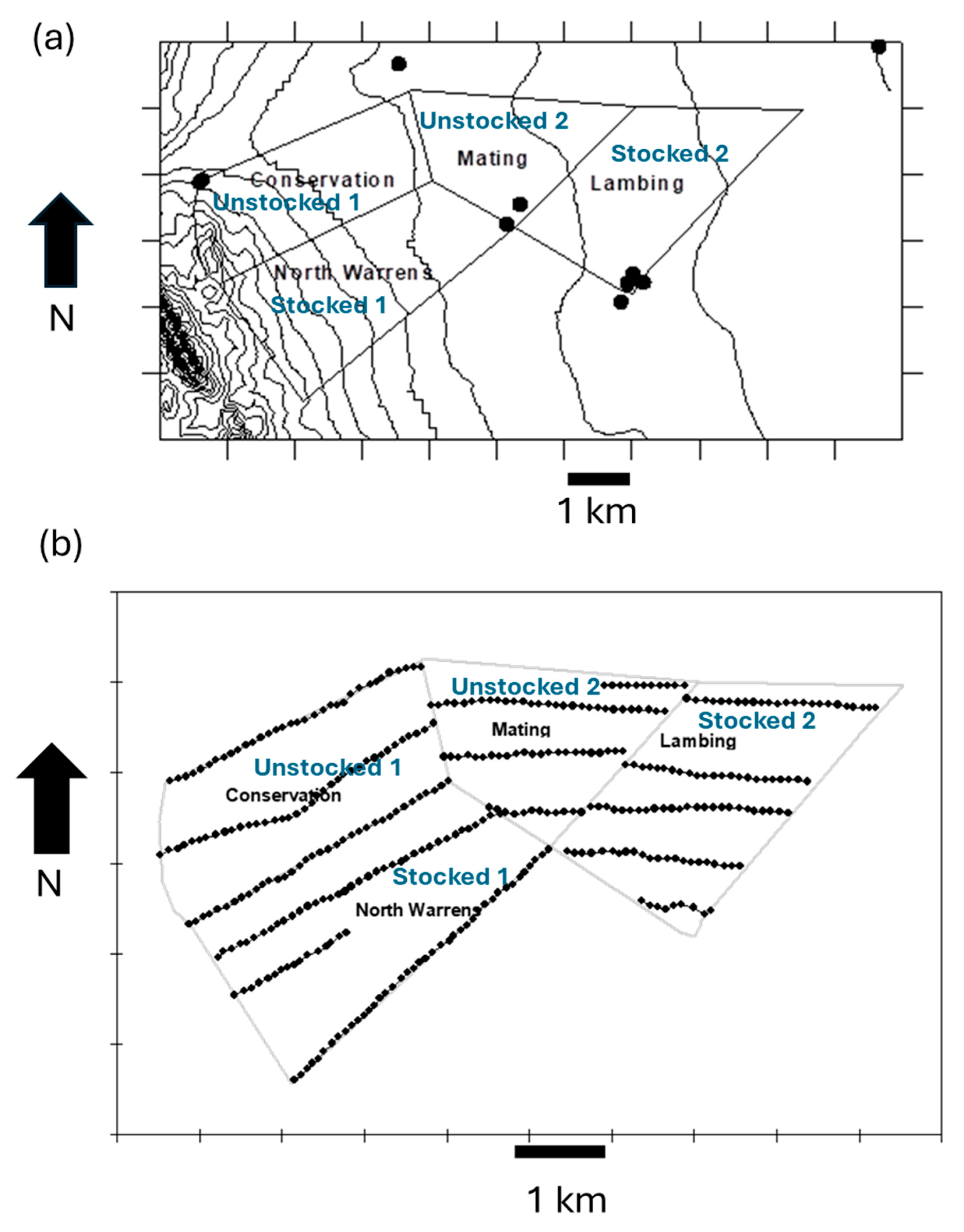
2.1. Study Site

The study was conducted at the University of New South Wales Arid Zone Research Station at Fowlers Gap (Lat. 31°05′ south, Long. 141°43′ east) in arid northwestern New South Wales, Australia. The station is in the sheep rangelands of Southern Australia (as defined by [11]) and has more than a 100-year history of grazing sheep (an introduced species). The climate is dry, mildly arid, with hot summers and mild winters [47] and no distinct rainfall season. The mean annual rainfall from the inception of daily measurement at the research station (1966) to the conclusion of data collection for this study (1997) was 243 mm, with a coefficient of variation of 55%. Rainfall is unreliable, erratic and often patchy across landscapes.

Hot summers and cool winters prevailed during the study. Monthly rainfall was sporadic in the first 15 months, but thereafter, it was relatively regular to the conclusion of data collection (Figure 1). Rainfall deficiencies (0 mm) were frequent in this first period but did not amount to a formal declaration of drought under the Australian Bureau of Meteorology’s definition (http://www.bom.gov.au/climate/drought/drought-definitions.htm, accessed on 4 November 2024). However, for brevity, we refer to this period of initial rainfall deficiency as ‘drought’. At inception, there was some overhang of pasture resources from preceding above-average rainfall.

This study centred on four adjacent paddocks on the eastern side of the 39,000 ha Station (Figure 2a). For reference to other studies at the station, the following paddock names are given: Conservation destocked for 30 y, North Warrens, Mating destocked for 10 y and Lambing. Further reference to paddocks is by their stocked condition: Unstocked 1 (Conservation), Stocked 1 (North Warrens), Unstocked 2 (Mating) and Stocked 2 (Lambing). Fences defined the boundaries of the paddocks and were constructed from high tensile wires, very strong end assemblies, widely spaced posts and long strains (Suspension Fence (2) in [48]). This design allowed lateral flexing when hit by stock, goats or kangaroos. The fences contained sheep but were porous to kangaroos (pushed under or jumped over), goats (pushed through or over) and rabbits (no barrier). Two paddocks, Unstocked 1 (520 ha) and Stocked 1 (647 ha), incorporated alluvial plains and the hillsides of the Barrier Range traversing Fowlers Gap. The other two paddocks, Stocked 2 (591 ha) and Unstocked 2 (400 ha), were situated exclusively on alluvial plains. The paddocks differ in stocking history and landscape; thus they are treated as two matched pairs in the results.

2.2. Landclasses

The study site comprised a mosaic of 20 landclass units with characteristic soil types and vegetation (see Figure 3 in [13]). Their descriptions are provided in Appendix A.

The soil profile of Stocked 2 and Unstocked 2 was texture contrast soils (or loamy sands), interspersed with light clays or heavy clays. Gilgais (small water-holding depressions), stony surfaces, channels and depressions were common. Erosion had produced large, scalded areas or clay pans. The micro-topography was a mosaic of water run-on and run-off areas where those adjacent to clay pans experienced high water run-on after rain and remained wet for long periods. The dominant vegetation types were cottonbush (Maireana spp.), saltbush/cottonbush (Atriplex-Maireana spp.) and copperburr/cottonbush (Sclerolaena-Maireana spp.) communities.

The lower halves of Stocked 1 and Unstocked 1 had landclasses like those in Stocked 2 and Unstocked 2. The soil profile was texture contrast/heavy clay soils, heavy clay depressions and degraded and scalded texture contrast/heavy clays. This supported cottonbush/saltbush vegetation. The soil profile of the topographically higher areas was desert loam soils and brown gibber (stony) soils, and the dominant vegetation was saltbush and bluebush (Maireana spp.).

2.3. Estimates of Mammalian Herbivore Densities

The methods, except for nighttime surveys, are described in detail in [13]. An abbreviated description is given here. The goal was to gain a regular estimate of the abundance of each of the seven focal species residing in the study site.

2.3.1. Kangaroos

Surveys were conducted in the middle of each month from April 1994 to March 1997. Abundance was estimated from counts taken along transects (Figure 2b) using the strip-transect method [49]. Strip width was 250 m to each side of a transect, set about 500 m apart, so that the whole of each paddock was effectively surveyed. The average flight distance from an ambulatory person or motor vehicle is around 80 m for red kangaroos and common wallaroos [50], so double counting was unlikely. We assumed that we detected and counted all individuals and that any bias was constant since the observer (IW) and transects were fixed. Surveys commenced within half an hour of sunrise (sunrise GMT+9.5 h: winter solstice 0701, summer solstice 0456), when kangaroos are active regardless of the season [51]. The observer rode a motorbike (Kawasaki 250KL, Tokyo, Japan) along transects at about 15 km h⁻¹. This type of vehicle is familiar in the study site as it has been used in livestock management and by researchers for several decades. All paddocks were surveyed twice—Unstocked 1 and Stocked 1 on day 1 and 3, Unstocked 2 and Stocked 2 on day 2 and 4. The direction of the duplicate surveys was reversed to remove bias from the time of day and angle to the sun. Species density per hectare was estimated from the average of both surveys. In total, 34 of the 36 scheduled monthly daytime population surveys were conducted. Two discontinuities occurred: the month 7 survey could not be carried out due to an injury sustained by the observer, and the month 24 survey was forgone due to very wet conditions in the paddocks, making transit impossible.

Observations were made from a stop at the nearest transect post using a pair of Permafocus binoculars (Jason 10 × 50, Permafocus 2000, Kansas City, MO, USA). A datascope (KVH Datascope, Middletown, RI, USA) was used to estimate the angle (from true north) and distance of subjects (±5 m at ≤100 m, ±10 m at >100 m) from the observation position. The observer’s position, distance and angle from the observer, species (red kangaroo, common wallaroo, eastern grey kangaroo, western grey kangaroo) and size/sex class, were recorded. The individual’s position was calculated for the Australian Map Grid using grid north and trigonometry. The abundance of each species was calculated on a 1 ha grid and overlaid on a raster map of landclasses to estimate habitat use at the paddock and the landclass within paddock levels.

Twice yearly, in winter and summer and in conjunction with day surveys, population counts were conducted on four consecutive nights starting about 2 h after sunset (sunset GMT+9.5 h: winter solstice 1709, summer solstice 1906). Each count was completed within about 3 h, and each paddock was surveyed twice. All kangaroos seen were counted using a 100 W spotlight from an elevated position on the tray of a 4WD utility truck, driven at approx. 15–20 km h⁻¹. The distance (±20 m) from the observer and angle (±10°) from the transect line to an individual or the first member of a group sighted, the group size and the species were recorded. At night, sightability decreased with increasing distance from the transect line and declined markedly beyond about 125 m (range of spotlight approx. 200 m). The data were therefore truncated to a strip of 250 m. The line transect estimates of kangaroo density were generated using the program TRANSECT based on [52], and the Fourier transformation estimator was employed because of pooling robustness and estimation efficiency. Six nighttime surveys were completed over the three successive winters and summers between 1994 and 1997.

Figure 2. (a) Four paddocks incorporating the study site. Curves represent 5 m contour lines, and solid circles (•) show stock watering troughs or earthen water tanks. (b) Transect lines traversing the study site. • = 100 m marker post.

Figure 2. (a) Four paddocks incorporating the study site. Curves represent 5 m contour lines, and solid circles (•) show stock watering troughs or earthen water tanks. (b) Transect lines traversing the study site. • = 100 m marker post.

The age and sex of red kangaroos at mortality were estimated from skulls collected during the study period. These were acquired whenever encountered during data collection in the paddocks, with the addition of paddock-wide grid searches at three-month intervals. The skulls were cleaned. The upper jaw was placed on a sighting device comprising a clear Perspex plate with a mark to align the zygomatic arch as a reference point and a perpendicular line to position the long axis of the skull should one arch be damaged. The number and parts of molars that progressed past the reference line were then expressed as a ‘molar index’. This molar index was then entered into a species-specific equation to calculate the age of an individual. For red kangaroos, the equation used was (after [53])

Log age (days) = 2.211 ± 0.3604 M.I. (M.I. = molar index)

In total, 175 red kangaroo skulls were collected. Of these, 103 were from mature females, 53 were from mature males, 13 were from mature individuals of indeterminant sex and 6 were from juveniles.

2.3.2. Sheep

The numbers and sex of sheep in Stocked 1 and Stocked 2 paddocks were set according to management decisions based on the history of the paddock, visual assessment of the vegetation resource base and Merino bloodlines. Flock size was counted on three occasions when sheep were mustered for shearing, lamb marking and crutching. The onset of lambing was recorded, and reproductive success was determined by dividing the number of lambs counted at lamb marking time (usually about 2 months after lambing started) by the number of ewes.

Three individual sheep were selected at random within each flock and marked. Their location during kangaroo surveys was estimated by simple trigonometry from the angle (from grid north) and distance (within 10 m) from the observer and the observer’s position (estimated from GPS reception) in Australian Map Grid coordinates. The flock was cohesive except during lambing when individuals or sub-flocks were counted. Sheep density was estimated on a 1 ha grid.

2.3.3. Rabbits

Rabbit warrens were located by an initial grid search and marked with orange flagging tape and their position estimated with a GPS receiver. New warrens were incorporated in follow-up surveys of each paddock at 3-month (mid-season) intervals when the number of active entrances for each warren was calculated. Population abundance was estimated from the following equation: number = 0.707 + 0.355x where x = number of active entrances [54]. This measure is conservative as it only includes adult rabbits. Ten rabbit warren surveys were conducted. The spring 1994 survey was foregone due to injury to the observer.

Warrens are point sources of rabbit activity. To estimate the spatial extent of rabbits, fluorescent powder tracking was conducted. Individual rabbits were captured using cylindrical wire mesh traps from warrens representative of the main landclasses, once during drought and once during average conditions. The captured individuals were thoroughly dusted in a bag with fluorescent powder and released. A UV light was then used 1–2 h before dawn in the night after capture to scan the ground for particles of the powder. The fluorescent tracks were followed, and the longest distance from the warren before rabbits returned to their burrow was marked and measured. The mean distances from a sample of several warrens and rabbits were estimated for the foraging radius. Custom software defined a circle around each warren with a radius defined by the maximum foraging distance, and the estimate of rabbit abundance at the warren was assigned to this polygon. Polygon vector-to-raster conversion produced a map of rabbit abundance and distribution on a 1 ha grid.

2.3.4. Goats

The abundance and location of goats were estimated during the monthly kangaroo population surveys. The density of goats on a 1 ha grid was estimated as for kangaroos.

2.4. Spatial Distributions of Herbivore Populations

The population here represents the individuals in the study site not the population at large. Locations were calculated in truncated Australian Map Grid coordinates 65xxxxx m north, 5xxxxx m east from an origin of 31°38′7″ south, 141°00′0″ east UTM. Conversion between geographic and grid coordinates followed the method of Geoscience Australia (https://www.geodesyapps.ga.gov.au/grid-to-geographic, accessed on 15 November 2024) for ellipsoid WGS84 and Zone 54. Population utilization distributions (PUDs) were generated from data sets of the locations for kangaroos using Anderson’s [55] Fourier transformation estimator. This non-parametric utilization estimator makes no a priori assumptions about the underlying distributions of the utilization shape [55,56], nor is it unduly influenced by sample size and outlying points. The intensity of use of an area is defined by a MAP value (minimum area versus probability). The area of most intensive use [57] or core area is estimated from the MAP(50) where there is a 50% probability of finding, in our case, an individual in the population of the herbivore species. The total area is defined by the MAP(95), the area with a 95% probability of finding an individual in the PUD. Using MAP(95) instead of a MAP(100) reduces the effect of outliers, which greatly decrease the precision of the area estimate [55]. The analysis concentrated on the MAP(50) core areas, a less biased measure of the changing space use pattern than the MAP(95) total home range area.

Custom software was used to generate the MAP(50) and MAP(95) values. This software produced a file of location probabilities compatible with the grid file format of SURFER V6.01 (Golden Software Inc., Golden, CO, USA) that was used to plot PUDs.

A measure of the intensity of use of each paddock (HAB) by kangaroos and other species in the study site was derived from

HAB(50 or 95) = MAP(50 or 95) area/paddock area

The MAP(50) and MAP(95) estimates were constrained so that only those 1 ha blocks falling within the paddock boundary were used.

The MAP and HAB(50) and MAP and HAB(95) of sheep were calculated from data sets of locations combined from population surveys and radio-tracking locations (see Section 2.10 below). The number of locations for goats was too few to calculate unbiased PUDs. For rabbits, their density within their foraging radius from every warren was equated to the core area of the rabbit populations and used as an equivalent to the MAP or HAB (50) area of other herbivores’ PUDs.

2.5. Statistical Analysis

Most statistical analyses were performed with SPSS for Windows version 9.0 (SPSS Inc., Chicago, IL, USA) or custom software (developed by DBC). Multivariate analyses were repeated using SPSS for Windows version 17 to provide a better resolution of statistical power and compliance with test assumptions. Non-parametric tests were used when the assumption of normality or homogeneity of variances was not met. The central tendency is presented as mean ± 1 standard error (SE) for parametric tests, or median and interquartile range (IQR) for non-parametric tests.

2.6. Analysis of Spatial Distributions

In general, the density and distribution results were analyzed on a 1 ha grid through the creation of Idrisi image files (Idrisi GIS for Windows V2, Clark Labs, Worcester, MA, USA). Idrisi image layers for the boundaries of paddocks and landclasses within paddocks were used to divide the results for the study site on a finer spatial scale and to relate density to habitat types (i.e., landclasses). Several types of analyses were used to assess habitat preferences. HAB(50) and HAB(95) PUDs were regressed against biomass (total, pasture and green pasture, grass and green grass, forbs and copperburrs—methods to estimate biomasses in [13]) to discover associations between PUDs and vegetation availability.

2.6.1. Landclass Selection

The available habitat at the study site was assessed based on the landclasses available. The study site comprised a mosaic of 20 landclasses, some of which overlapped the different paddocks. Unstocked 1, Stocked 1 and Stocked 2 were characterized by 7 landclasses and Unstocked 2 by 8 landclasses.

The selection of landclasses by herbivores was calculated using custom software to determine significant deviations from random distributions and selection ratios based on the methods of Manly et al. [58]. The application used log-likelihood chi-squared tests to determine (a) if the distribution of the herbivore species was similar on all surveys (L1), (b) if the herbivore species (surveys are pooled) selects landclasses in proportion to their availability (L2) and (c) if the herbivore species on average selects landclasses in proportion to their availability (L1–L2). The ‘selection ratio’ (SR) for each landclass used was calculated from the ratio of the proportion of the population of the herbivore species on the landclass and the proportion of that landclass in the total habitat used (or surveyed). Ninety-five percent confidence intervals (CIs) were used to distinguish significant selection for or against landclasses by the different species, where SR + CI < 1 was significant selection against the landclass, and SR-CI > 1 was significant selection for the landclass, else the landclass was selected in proportion to its availability or not used (SR = 1).

A contingency analysis was used to compare the frequency of individuals in landclasses in the day and night surveys. Standardized residuals were calculated to identify the source of any significant differences.

Multi-dimensional scaling (MDS) was used to establish associations between the populations of the various herbivores and the landclasses characterized by important vegetation categories and underlying soil types. MDS constructs a ‘map’ showing the relationship between a number of objects—here, the herbivore species is based on their relative usage of landclasses in the study site [59]. Since MDS examines matrices of dissimilarities, the resultant map shows the relative separation of the herbivores across the landscape in the study site.

Habitat preferences were also examined by correspondence analysis (CA). CA was applied as an additional measure to test similarities and/or dissimilarities of the species in space over time. The method provides an ordination of n sites (here landclasses) based on the abundance of p species (here herbivore densities and vegetation biomass) [59]. CA was used to choose species and site values that were as highly correlated as possible, so CA gives a simultaneous ordination of species and sites. CA gives more weight to rarer species than MDS.

A combination of different analytical approaches helps overcome the limitations inherent in each analysis [60]. For both MDS and CA, 11 population surveys were used. These surveys corresponded to the rabbit surveys undertaken.

2.6.2. Other Habitat Features

A digital terrain model was constructed using Tosca 2.0 (Clark Labs, Worcester, MA, USA), an application that digitizes paper maps from a graphic tablet. Contours (5 m levels Above Sea Level—ASL), man-made drainage channels, natural erosion gullies and creek lines were digitized as vectors from the Fowlers Gap 1:25,000 topographic map (Department of Lands 1971). The vectors were converted to a 1 ha grid raster map using Idrisi. Similar maps were made of the fences that bounded paddocks, but the coordinates were measured using a GPS receiver. The resultant polygons were converted to 1 ha raster maps of the areal extent of each paddock.

The maps of contours, drainage channels, erosion gullies and creek lines and the tree density maps were overlayed onto species distribution maps to look for habitat segregation with respect to conspicuous environmental features.

2.7. Overlap of Species’ Population Home Ranges

The overlap of the utilization distributions of two populations was examined. The population utilization distributions (PUDs) were cross-tabulated using a custom software application to calculate the percentage of the MAP(50) and MAP(95) that was shared between species. This was expressed as the percentage of the total area encompassed by species A and B that was common to both. The analysis was applied to three periods of 12 months, for which the monthly population survey data were pooled, and each paddock was then analyzed for those herbivores abundant enough to have warranted the establishment of PUDs.

2.8. Species Richness in Space and Time

A custom software application was used to derive the average species richness in each hectare block for each season. This required the determination of the presence of one or more individuals of the seven herbivore species in a hectare block during a population survey. The presence values for each survey were summed to give a richness value, and the results for the two replicated surveys were averaged.

These species richness maps were compared to ones derived from a random distribution model using a contingency analysis on the frequency of 1 ha blocks with a richness of 0 through to 7. The random distribution model maps were created by using the abundance of each species on a population survey and distributing these individuals into 1 ha blocks in the study site at random for 10,000 simulations. The expected richness was the average for these simulations.

2.9. Determinants of Densities and Distribution of Resident Herbivores Across Landclasses

Multiple regression analysis was applied to discover the most important relationships between resident herbivores and variables describing their habitat. These variables were densities of the other mammalian herbivores in the study expressed as number ha⁻¹. Vegetation variables, all expressed in biomass (kg) ha⁻¹, were pasture and its components (copperburrs, forbs and grasses) as either total or green biomass, forbs and grasses combined, germinating grasses, RLC (round-leafed chenopod shrubs), FLC (flat-leafed chenopod shrubs) and total ground vegetation (pasture and shrubs) (see [13] for methods relating to vegetation variables). The densities of trees (alive or dead in three height categories 1, 2, 3+ m), slope and water distance (m) completed the list of variables regressed.

Plots of the dependent variable on each independent variable were examined in all analyses to look for non-linear relationships. No transformations of the data set were deemed necessary.

2.10. Spatio-Temporal Behavior of Individuals

To examine the spatio-temporal behaviour of herbivore species at the individual level, a sample of mature female red, eastern grey and western grey kangaroos and sheep (ewes) was captured, radio-collared and radio-tracked.

2.10.1. Capture and Radio-Collaring

Red and grey kangaroos were caught by cannon-netting [60] at water troughs during warm, dry periods or by ‘stunning’ [61] in winter. The cannon net comprised a 25 × 25 m rope mesh net with the leading edge carried by five equally spaced projectiles. The projectiles were fired by an 8 g charge of black gunpowder that was packed into a 12-gauge shotgun case. A matchstick detonator was inserted into the brass-cased end and detonated electronically from a vehicle parked 30–50 m away so that the net shot over the trough. Kangaroos that had bent down to drink were then entangled beneath the net to effect capture. ‘Stunning’ involved locating a suitably sized kangaroo by spotlighting from the tray top of a 4WD truck at night. When the kangaroo stopped and was mesmerized by the spotlight, a high velocity bullet (.22 calibre) was fired between the kangaroos’ ears, just above its skull. The shock wave of the bullet temporarily impaired the hearing of the kangaroo, and this and the strong light disoriented it, allowing runners to effect capture

Upon capture, kangaroos were placed into large sacks and were sedated with an intramuscular injection of Valium (Roche Holding AG, Basel, Switzerland) at a dosage of 1 mg per 10 kg of body weight as a precaution against capture myopathy [62]. All kangaroos were weighed to the nearest 0.5 kg and a standard set of skeletal measurements (foot, arm, leg length) and tail butt circumference were recorded. The reproductive status of females was assessed by checking for pouch young (PY) or the presence of capped (indicating immature females) and elongated (indicating lactation for young-at-foot) teats. The size (foot or body length, and weight if furred and out of the pouch) and sex of pouch young were recorded. The sex of young-at-foot (YAF), if identified, was recorded, and if captured, they were processed like adults.

Only adult females were radio-collared. These are the most sedentary part of the population [32] and hence most likely to provide the best information on habitat selection and movement of individuals independent of mate-searching behaviour (cf. large males) or juvenile dispersal. Adult females were fitted with custom-made collars carrying radio-transmitters with a unique frequency (Models MMK5, 6 or 7 Telonics Inc., Mesa, AZ, USA) for use in the individual home range studies. The transmitters usually had a 3 y battery life and weighed ~250 g (1% of average body weight). All kangaroos captured (cannon-netting often led to multiple captures, not only the target animal) were also fitted with a uniquely numbered Allflex disk ear tag (Allflex Australia Pty Ltd., Murarrie, QLD, Australia); females were tagged in the left ear and males in the right ear. Recaptured animals were fitted with an additional tag in the other ear.

Thirty-four red kangaroos, 15 western grey kangaroos and 5 eastern grey kangaroo females were fitted with transmitters out of a total of >100 captures of both sexes and all species. The initial effort aimed to radio-collar six red kangaroo females in each paddock and 12 eastern grey and 12 western grey kangaroo females across the study site. The sampling of eastern grey kangaroos was reduced when it became apparent that they were transient in the study site.

2.10.2. Radio-Tracking

Radio-collared subjects were tracked on a weekly basis, either during early morning or late afternoon. A handheld receiver (Model RX 8910, Televilt AB, Lindesberg, Sweden) or a handheld directional antenna (Model RA-2A, Telonics Inc., Mesa, AZ, USA) attached to a scanner/receiver (Model TS-1 and TR-2E, Telonics Inc., Mesa, AZ, USA) were used to locate the signals emitted from each subject’s transmitter. The subject was then approached as far as possible on a motorbike or on foot until good visual contact was made using binoculars. The location of the animal was then determined by simple trigonometry using a GPS (Pronav GPS 100, Garmin Corp., Olathe, KS, USA) to determine the observer’s position and a digital compass and rangefinder (KVH Data Scope, KVH Industries, Middletown, RI, USA) to determine the subject’s angle and distance from the observer. The current reproductive status of each subject was recorded according to whether she had a PY and/or was accompanied by a YAF whose sex was determined. If the female was a member of a group (including all other conspecifics within 50 m—[63]), then all individuals in the group were also counted and their size/sex class and reproductive status were determined.

Few individuals were tracked for the whole of the study (

Table 1. Average weight (kg), number of locations and days tracked of female kangaroos fitted with radio-transmitters.

	Red Kangaroos (n = 34)	Western Grey Kangaroos (n = 15)	Eastern Grey Kangaroos (n = 5)
Mean weight ± SE Range	27.1 ± 0.6 21–33	26.5 ± 0.7 23.5–34	24.7 ± 0.9 23–28
Mean locations ± SE Range	69 ± 6 9–133	81 ± 12 10–140	72 ± 25 10–140
Mean days tracked ± SE Range	562 ± 51 90–1023	612 ± 86 63–1023	537 ± 191 68–1005

). Mortality and emigration, particularly during the drought, forced the capture effort to continue throughout the second year of the study to maintain an adequate sample through the replacement of dead or lost individuals.

2.10.3. Data Handling

The home range of each kangaroo subject was established using Anderson’s [55] non-parametric Fourier transformation estimator. A grid size of 1 ha was used to be consistent with the mapping of population densities; vegetation cover, biomass and greenness; and geographic features in Idrisi for Windows V2. A custom software application was used that calculated the area of the MAP(50) and MAP(95) distributions, representing core and home range areas, respectively. The application outputted a file of the coordinates of grid squares within the MAP(50) and MAP(95) ranges and a grid file of probabilities under the smoothed utilization distribution compatible with Surfer 6.0 (Golden Software, Golden, CO, USA). The coordinate file for each subject was cross-tabulated with Idrisi image files containing geographic features of the study site; the abundances of the seven mammalian herbivores and vegetation characteristics spanning the period the subject was radio-tracked (

Table 2. Variable set used in analyses of home range quality.

Habitat Characteristic	Variable 1
Geographic	Slope (contour at 5 m intervals ASL)
	Distance from water (m)
Vegetation 2	Tree density (number ha−1)
	Proportion of green grass biomass
	Proportion of green forb biomass
	Copperburr biomass (kg ha−1)
	Flat-leafed chenopod biomass (kg ha−1)
	Round-leafed chenopod biomass (kg ha−1)
Herbivore density	Red kangaroo (abundance ha−1)
	Western grey kangaroo (abundance ha−1)
	Common wallaroo (abundance ha−1)
	Sheep (abundance ha−1)
	Rabbit (abundance ha−1)

¹ All variables were calculated as the proportional difference in the mean for the individual’s home range to the mean for the study site. ² See [13] for the calculation of vegetation variables.

).

Since subjects were not all tracked contemporaneously, due to mortality and the vagaries of capture effort, maximum use of the data was made by calculating both the average absolute qualities of the home range and the relative qualities compared to the study site across the same time span. Since grass and forb biomasses were highly variable across the study, the key dietary components, green grass and green forbs, were expressed relative to the total biomass of that item rather than in absolute terms. Further, some locations for some individuals fell outside the study site, and the total number of locations varied between individuals. Therefore, covariates or weighting variables that expressed the proportion of home range or core area within the study site and the number of locations were used, where relevant, to account for this variation.

2.10.4. Other Mammalian Herbivores

For the remaining four species of mammalian herbivore in the study site, only sheep were tracked in a comparable manner to that of the kangaroos. A sample of three sheep in Stocked 1 and Stocked 2 were initially fitted with transmitters of the same kind as those used on kangaroos. However, the signal quality was poor, and the sheep proved easy to find since they were contained within paddock boundaries, generally moved as a large cohesive and conspicuous flock and tended to show routine patterns in their movement. Thus, the transmitters were removed, the sheep subjects were conspicuously marked and they were located by sight. Assessment of the movement patterns of these marked sheep was interpreted as representing the flock, as they were rarely separated from it except when ewes dispersed at lambing.

Common wallaroo females were not radio-collared because they were rare in the study site, preferring habitat in the hills or steeper slopes [37,64]. Hence, assessment of spatio-temporal interactions with other herbivores was restricted to the population level.

Goats were expected to be transient in the study site, since it contained little of their preferred habitat of steep wooded slopes and ridges. Furthermore, goats were known to range widely in Fowlers Gap [65] and other arid lands, with home ranges as large as the property area [66]. Thus, like common wallaroos, individual goats were not radio-tracked, as the effort was expected to have little return at the study site.

Rabbits were clearly sedentary and bound to their warrens. Their habitat selection was easily followed by surveying their activity in space and time with respect to their permanent shelters. Radio-tracking individuals was therefore deemed unnecessary.

2.11. Animal Ethics

This study was conducted under approval by the Animal Care and Ethics Committee of the University of New South Wales, Sydney—Approvals ACE 94/5 and ACE 96/139. Further approval was granted by the New South Wales National Parks and Wildlife Service to conduct scientific research on protected wildlife, namely four kangaroo species.

3. Results

3.1. Variation in Density of Herbivores in the Study Site

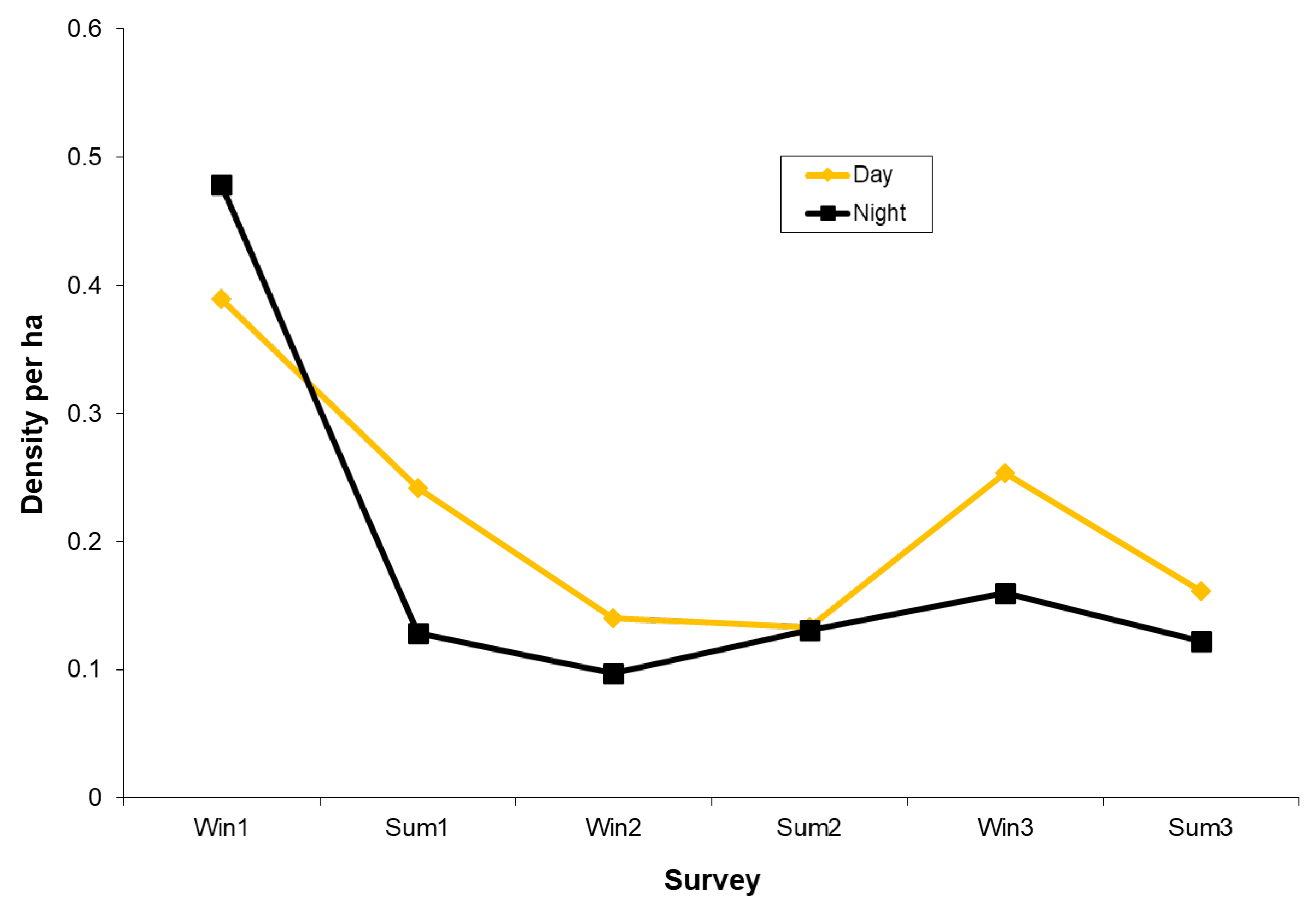
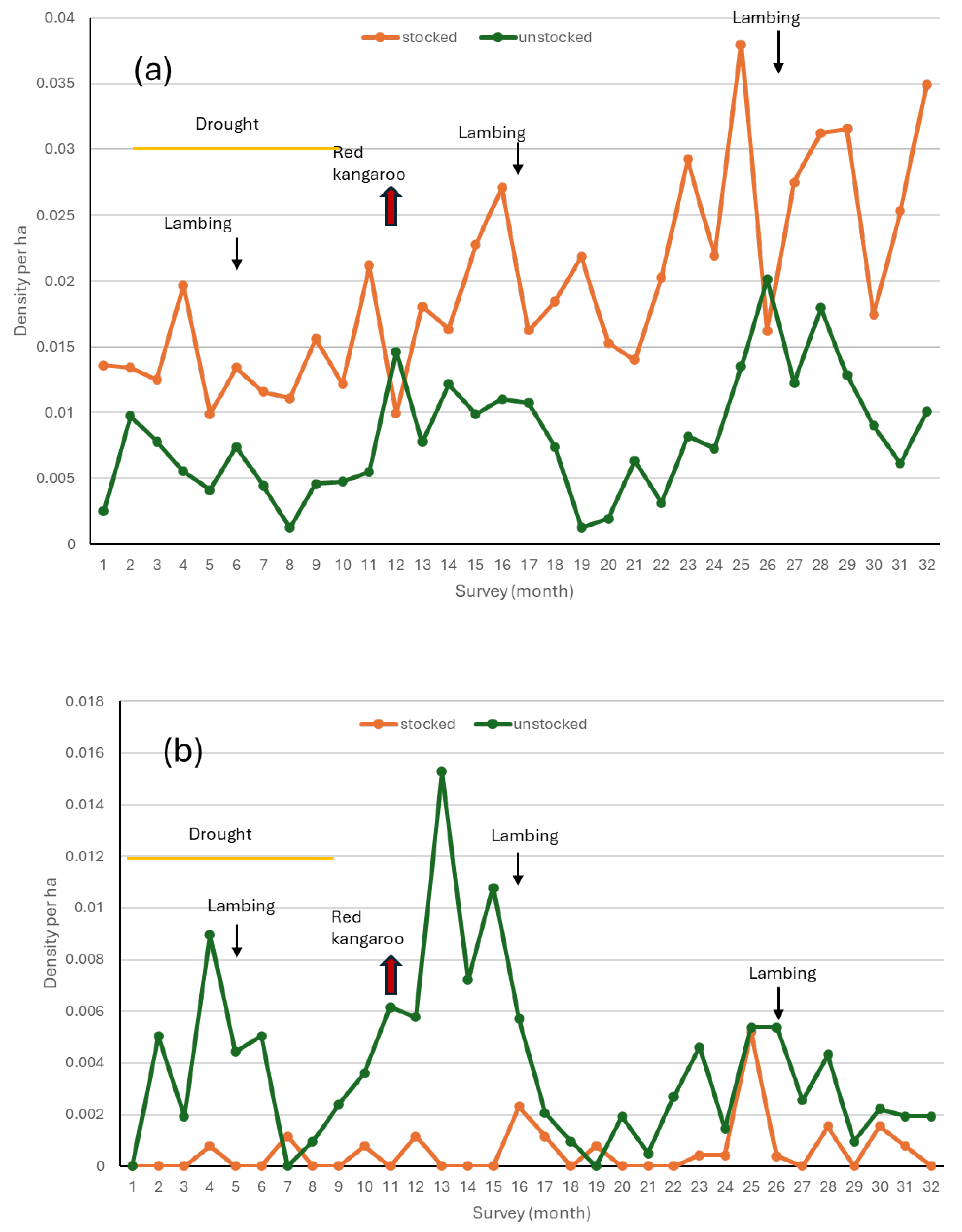
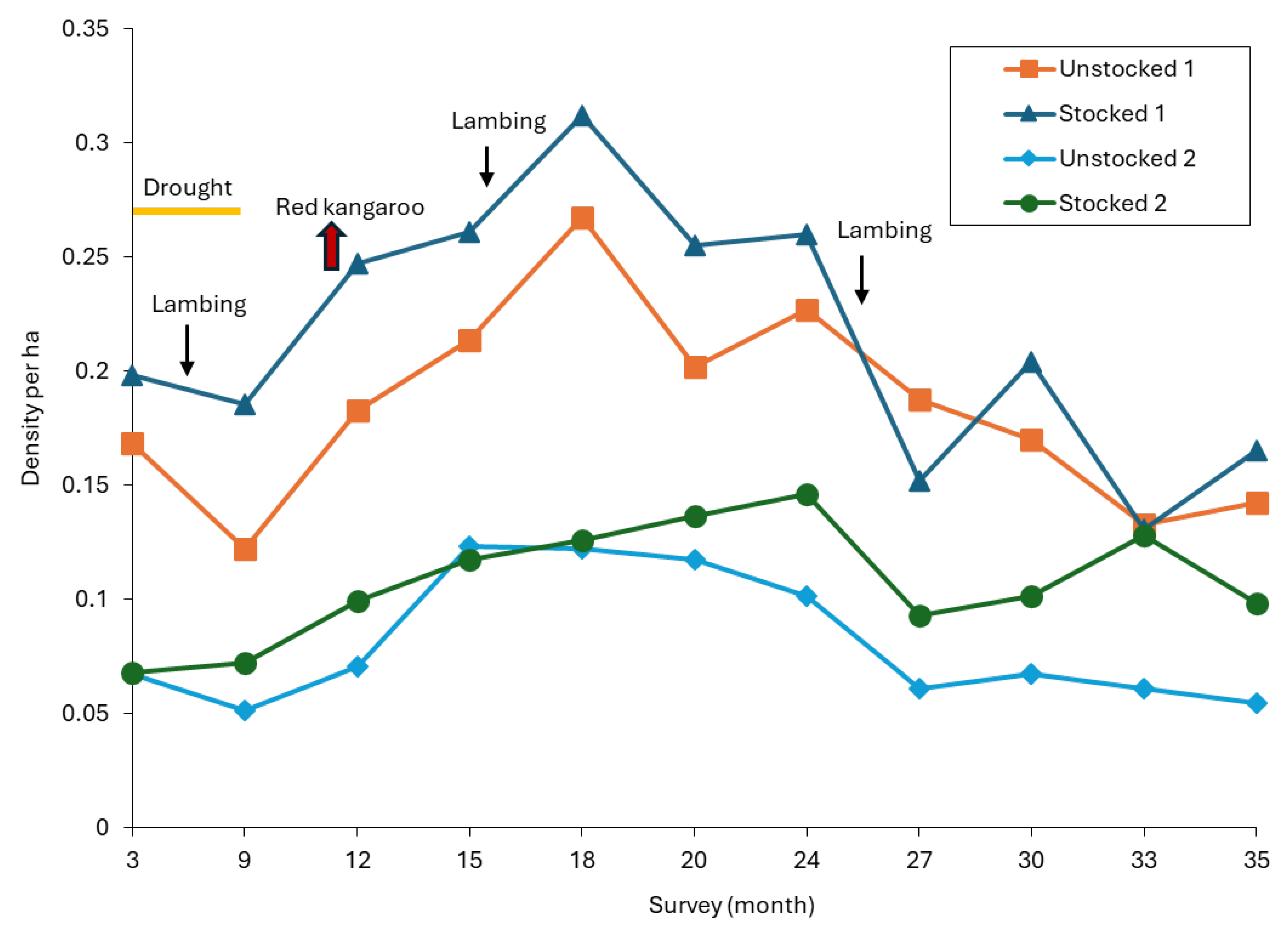
3.1.1. Density of Red Kangaroos

The density of red kangaroos on the entire study site averaged 0.25 ± 0.04 individuals ha⁻¹ (range: 0.11–1.18 ha⁻¹, n = 34). The unstocked paddocks carried significantly (Wilcoxon signed-ranks test, Z = −4.317, p < 0.001) higher densities of red kangaroos throughout the study period than the stocked paddocks (Figure 3). Unstocked 2 had a significantly higher density of red kangaroos than Unstocked 1 (Wilcoxon signed-ranks test, Z = −4.161, p << 0.001). The stocked paddocks had similar red kangaroo densities (Wilcoxon signed-ranks test, Z = −0.767, p = 0.443). The median density was 0.23 (IQR 0.19–0.30) ha⁻¹ for the unstocked paddocks and 0.15 (IQR 0.11–0.20) ha⁻¹ for the stocked paddocks.

Two events were indicative of the mobility of the red kangaroo population. Firstly, in surveys 10 and 11, a very large influx of red kangaroos from the surrounding area occurred, following a patchy, localized rainfall event after drought. The two exceptional counts represented a transient peak for all paddocks, relating to a density of almost two individuals ha⁻¹ in the unstocked paddocks (Figure 3). These numbers did not persist, and the densities dropped off again to pre-influx levels in survey 13.

Secondly, both stocked paddocks had a decrease in red kangaroo density at the onset of lamb dropping time (Figure 3) when ewes dispersed individually across the paddock. The density in the stocked paddocks remained relatively low, while lamb dropping continued and increased only after the lambing period had finished and the flock was cohesive once more. The decrease in red kangaroos in the stocked paddocks at these periods coincided with a distinct increase in the unstocked paddocks.

Thus, the proportional change in red kangaroo density between the months prior to lambing and the months incorporating the lamb drop was calculated for each stocked and unstocked paddock (Figure 4). Values in each of the three years were tested in a paired analysis with Stocked 1 paired to Unstocked 1 and Stocked 2 paired to Unstocked 2 in relation to the largest common boundary. The proportional change in the density of red kangaroos in the stocked paddocks was significantly higher than in the unstocked paddocks (Wilcoxon signed-ranks test, Z = −2.201, p < 0.05). Lambs were removed at shearing, so a similar analysis was undertaken using the month prior to (ewes + lambs) and following shearing (ewes). There was a significant proportional increase in red kangaroo density once lambs were removed in stocked paddocks relative to counterpart unstocked paddocks (Wilcoxon signed-ranks test, Z = −2.201, p < 0.05). In contrast, no proportional change in red kangaroo density was detected between consecutive months when no reproductive event or other disturbance related to sheep management occurred (Wilcoxon signed-ranks test, p > 0.05).

Densities in the stocked paddocks varied slightly more than in unstocked paddocks (stocked: CV (coefficient of variation) = 45.1%, unstocked: CV = 41.7%). The variation was most pronounced between the two ‘plains’ paddocks, with coefficients of variation of 42.0% (Unstocked 2) and 64.3% (Stocked 2), respectively. Densities in Unstocked 2 were also significantly higher than in Stocked 2 (Wilcoxon signed-ranks test, Z = −4.515, p << 0.001).

The density estimates were not biased by the time of counting. The densities for day and night surveys were strongly correlated (r = 0.9, p < 0.05) (Figure 5) and not significantly different (Wilcoxon signed-ranks test, Z = −1.363. p > 0.05). The night counts tended to be lower than the day counts, but such differences were small and inconsistent.

The red kangaroo population was typically dominated by adult females (i.e., females of reproductive age) at around 50% of individuals, with about 25% adult males (i.e., those classes bigger than adult females) and 25% immature red kangaroos (young-at-foot and juveniles of both sexes). The higher density of red kangaroos in unstocked versus stocked paddocks was consistent across these three age/sex classes (

Table 3. Mean (±SE) densities (individuals ha⁻¹) of adult females, adult males and juvenile/young-at-foot in unstocked and stocked paddocks.

Size/Sex Class	Unstocked	Stocked	p
Adult female	0.14 ± 0.01	0.08 ± 0.01	***
Adult male	0.06 ± 0.01	0.04 ± 0.01	*
Juvenile/YAF	0.05 ± 0.01	0.03 ± 0.01	***

Wilcoxon signed-ranks test (n = 33), * significant at p < 0.05, *** significant at p < 0.001.

).

3.1.2. Density of Eastern and Western Grey Kangaroos and Common Wallaroos

Red kangaroos dominated the study site, and the other three species of macropods were much less abundant. Contrary to red kangaroos, the second most abundant species, the western grey kangaroo, was at a significantly higher density in the stocked than the unstocked paddocks (Wilcoxon signed-ranks test, Z = −4.112, p < 0.001) (Figure 6a). Eastern grey kangaroos were at low densities but, like red kangaroos, were more abundant in the unstocked paddocks (Figure 6b). Consistent with their habitat preferences, common wallaroos were at significantly higher densities in the slope paddocks (Unstocked 1, Stocked 1) than the plains ones (Unstocked 2, Stocked 2) (Figure 6c). Even so, consistent with red kangaroos, common wallaroos were more abundant in Unstocked 1 than Stocked 1 (Wilcoxon signed-ranks test, Z = −1.923. p = 0.054).

3.1.3. Density of Rabbits

Like common wallaroos, significantly higher densities of rabbits occurred in the two slope paddocks than in the two plains paddocks (Friedman Test, χ² = 27.764, p << 0.001) (Figure 7). The rangelands do not support dense surface cover, so rabbits construct underground warrens for shelter. However, soils with a high clay content are not suitable for warrens. These soils may become waterlogged after heavy rainfall and then easily collapse, or these soils become very hard to burrow in during prolonged dry and hot conditions [67]. Thus, soil type is a useful explanatory variable for rabbit distribution, so landclasses (soil type and dominant vegetation type) were pooled into their base soil type—desert loam, brown gibber, texture contrast, texture contrast/heavy clay or heavy clay.

Unstocked 2 and Stocked 2 were in the flood plains with mostly texture contrast/heavy clay soils that were unsuitable for warrens. Warrens were mainly located along drainage channels that had been deepened by bulldozing, which created banks of friable soil. Unstocked 1 and Stocked 1, on the other hand, had much larger expanses of suitable brown gibber and desert loam soil.

The average density of rabbits on each of the five soil types was compared to the area of these soils using the methods of Manly et al. [58]. Rabbits significantly selected for desert loam (selection ratio ± 95% confidence interval = 1.54 ± 0.04) and brown gibber (3.77 ± 0.08) soils and against texture contrast (0.36 ± 0.01), texture contrast/heavy clay (0.38 ± 0.02) and heavy clay (0.33 ± 0.11) soils. Thus, the dispersion of rabbits in the study site was principally a result of variation in soils rather than other biotic or abiotic factors.

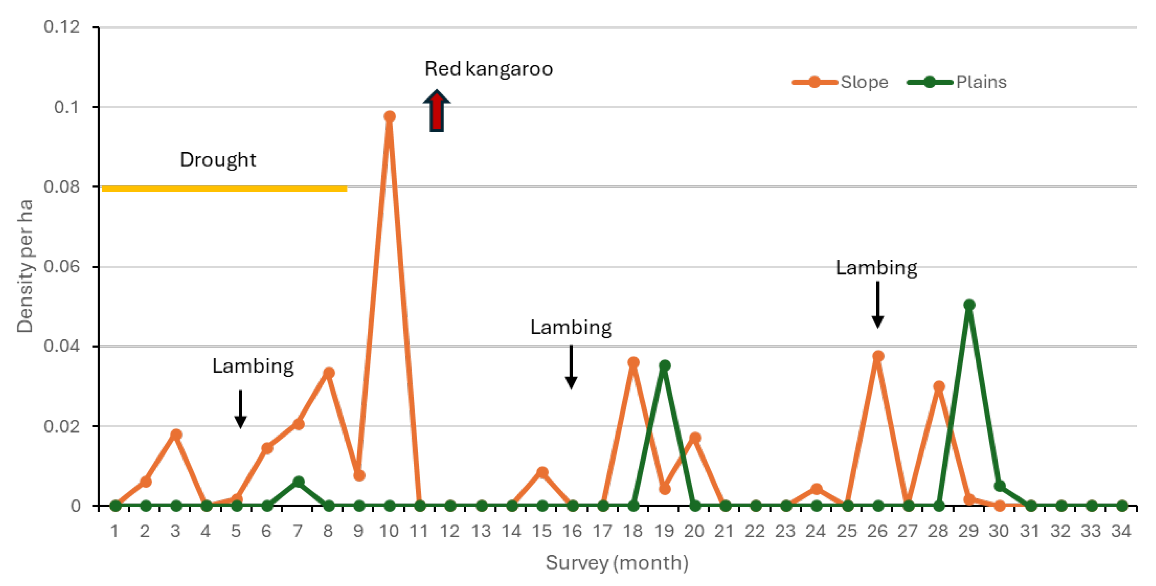
3.1.4. Density of Goats

Sightings of goats were irregular. Like common wallaroos, goats were at significantly higher densities in the slope paddocks, Unstocked 1 and Stocked 1, than the plains ones, Unstocked 2 and Stocked 2 (Wilcoxon signed-ranks test Z = −2.154, p < 0.05) (Figure 8). The only watering point on the slopes, a livestock trough, was adjacent to the northwest boundary of Unstocked 1 (Figure 2a) and attracted goats to this paddock.

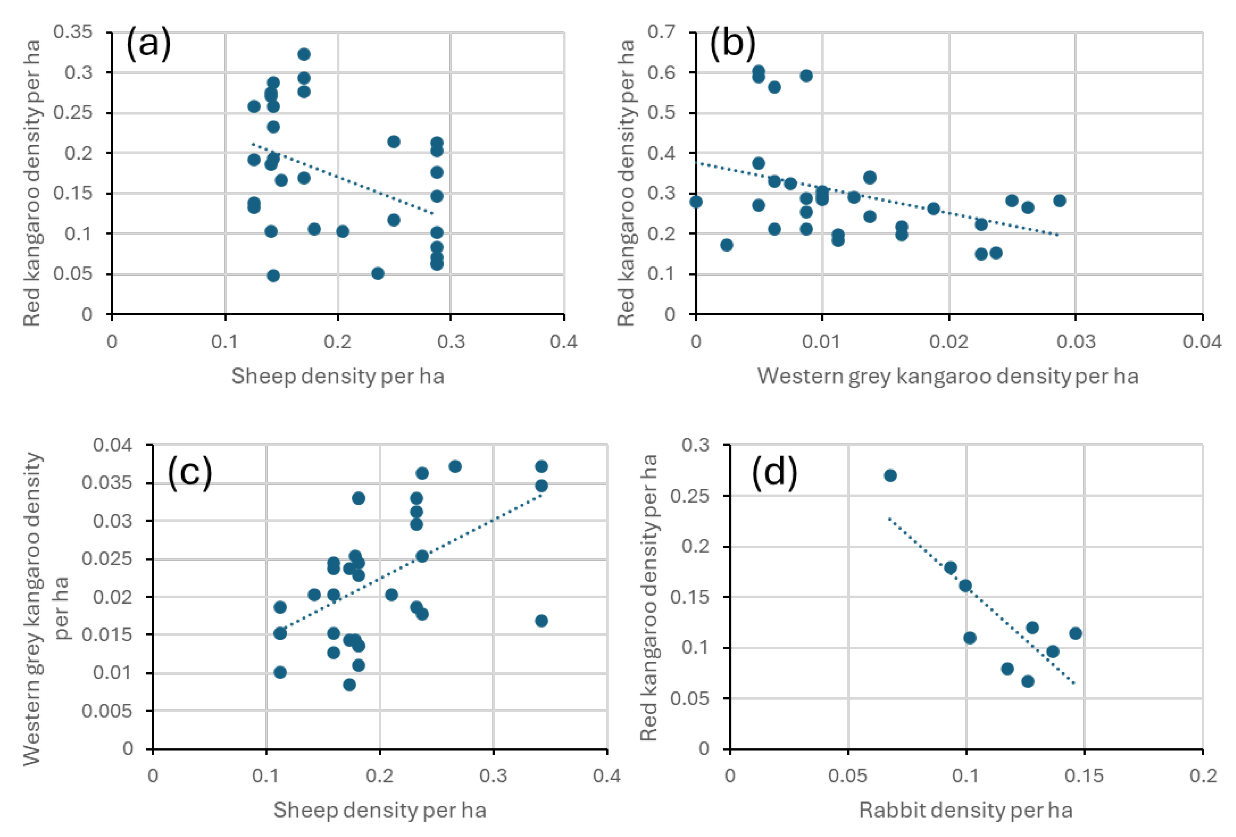
3.2. Correlations Between the Herbivore Populations

The relationships between the variation in the densities of relevant subsets of herbivores in each paddock were examined by simple correlation (Appendix B). The peaks in surveys 10 and 11 were removed for the red kangaroo sample and treated as outliers. Few species showed any significant synchrony/asynchrony in their population densities. The variation in sheep density was stepped with minor losses through mortality between shearing to lambing and lambing to shearing. Even so, red kangaroo densities were significantly negatively correlated with those of sheep in Stocked 1 (Figure 9a) with a similar weaker trend in Stocked 2. In Unstocked 2, western grey kangaroo and red kangaroo densities were significantly negatively correlated (Figure 9b). In Stocked 1, the variation in the western grey kangaroo density was unrelated to sheep but was significantly correlated in Stocked 2 (Figure 9c). The only other significant relationship was a negative one between rabbit and red kangaroo densities in Stocked 2 (Figure 9b). This was a general but weaker trend across all paddocks.

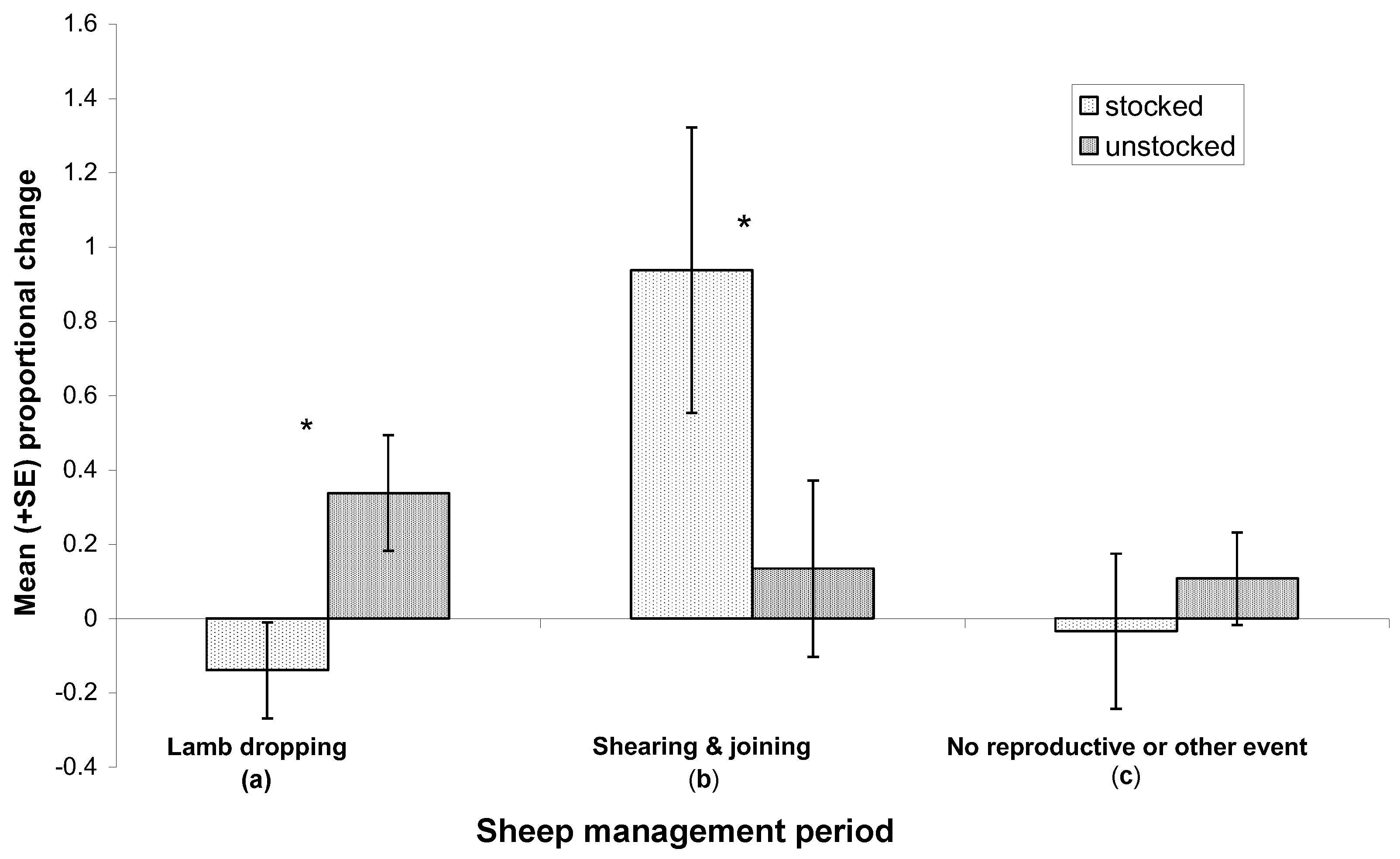
3.3. Reproductive Success and Mortality

The reproductive success of red and western grey kangaroos was estimated from the proportion of adult females with young-at-foot sighted in the population surveys. The reproductive success of sheep was estimated as the proportion of lambs to ewes at lamb marking (about one month after birth). The reproductive success of red kangaroos was not compromised by the presence of sheep, as there was no significant difference between stocked and unstocked paddocks (Paired t-test, t₃₁ = −0.083, p = 0.93) (Figure 10). The same relationship was found in western grey kangaroos. However, western grey kangaroos had a higher reproductive success than red kangaroos, and sheep outperformed both species (

Table 4. Annual reproductive success of adult female red and western grey kangaroos and sheep.

Year	Red Kangaroo 1	Western Grey Kangaroo 2	Sheep 3
1	43	-	80
2	16	49	84
3	38	98	96

Twelve-month average of proportion of females sighted with young-at-foot divided by the expected proportion: P(red kangaroos) = 0.67 ¹, P(western grey kangaroos) = 0.5 ², expressed as a percentage. Lambs marked as a percentage of ewes stocked ³.

).

Only the mortality results of red kangaroos are presented. The cause was not determined. However, poor nutrition, following periods of low rainfall, is considered the primary cause of mortality [43]. Predation and disease might be facilitated by nutritional setbacks. The representation of juveniles (3%) in the skull collection was very small, even though juvenile mortality was likely high given low reproductive success (Table 4). Due to their small size, foxes (Vulpes vulpes) or eagles (Aquila audax) likely carried the carcasses of these individuals away before they were discovered. Several small, fresh carcasses, when found, had their head removed, indicating scavenging by foxes. Hence, juveniles were likely under-represented in the sample.

Age classes were pooled into individuals ≤3 y, 4–12 y and >12 y. These divisions corresponded to sexually immature or early breeding individuals, breeding individuals and old, potentially non-breeding individuals. Mortality was the highest in the oldest age group, more so for males than females, but the distributions did not differ significantly between sexes (χ² =1.23, df = 2, p > 0.05) (

Table 5. Percent mortality in three age classes of female (n = 103) and male (n = 53) red kangaroos (y = year).

Age Class	≤3 y	4–12 y	>12 y
Female	8	44	48
Male	4	28	68

). Mortality was higher in the unstocked paddocks over the entire study period, when mortality was adjusted for the average density of red kangaroos per stocked and unstocked paddocks. Approximately 30.1% of the red kangaroo population suffered mortality in the unstocked paddocks compared to 19.5% of the stocked paddocks. These values are probably underestimates since very young individuals are under-represented in the sample.

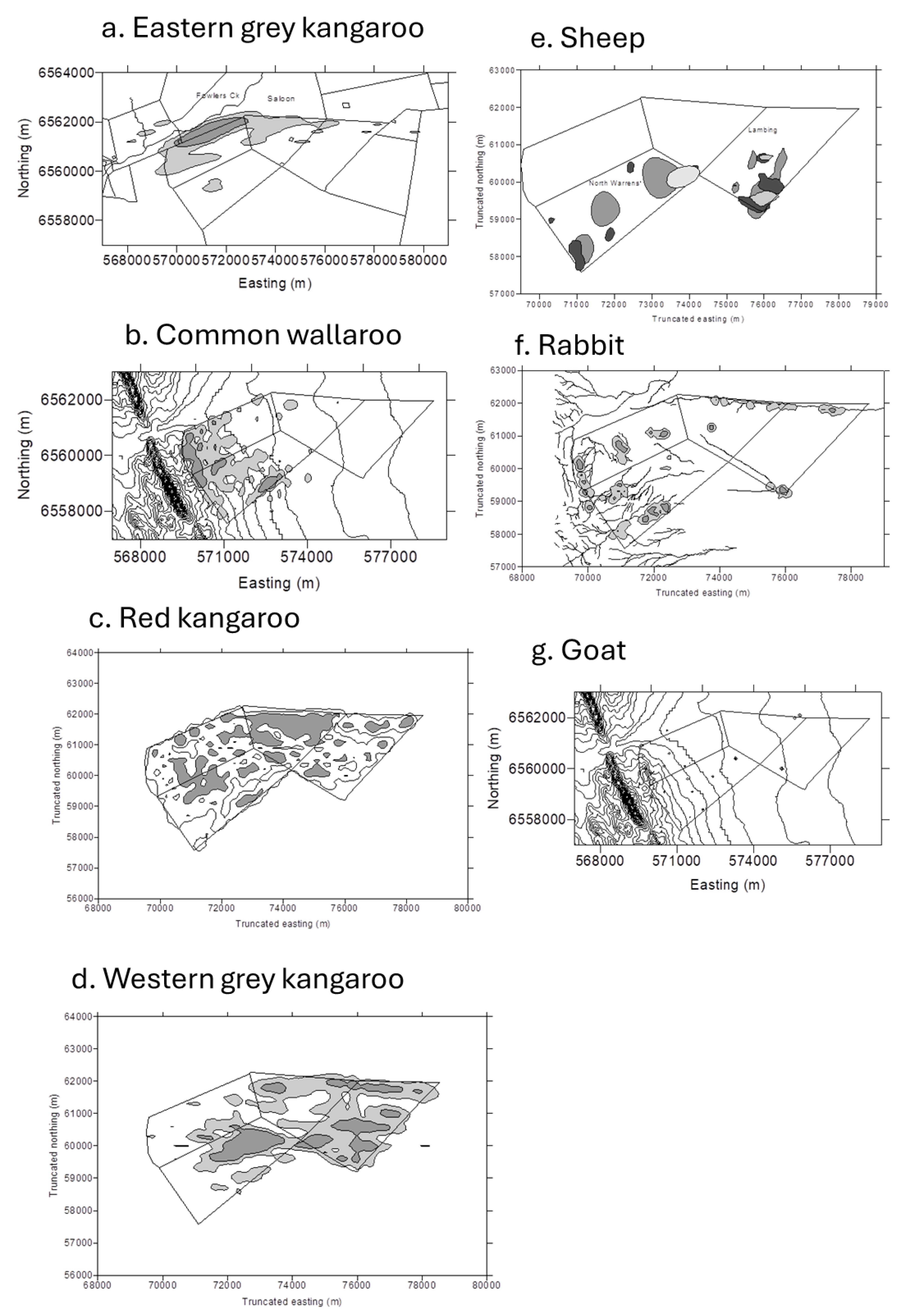
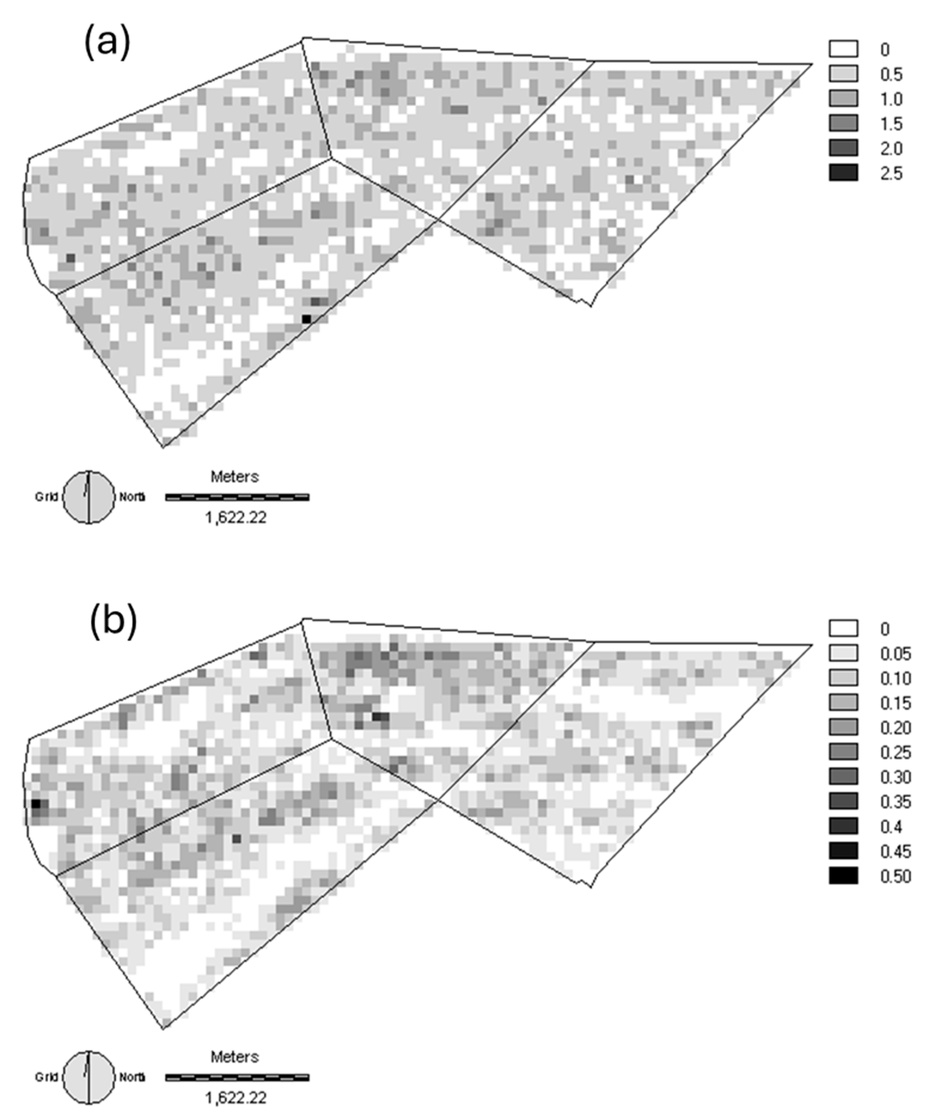
3.4. Population Utilization Distributions of Herbivores

Population utilization distributions were calculated for each monthly survey. The results presented here summarize the dispersion of each herbivore species across the 34 surveys (Figure 11).

Eastern grey kangaroos were the least abundant of the seven herbivores in the study site. They typically occupied habitat along the northern boundaries of Unstocked 1 and Unstocked 2 towards Fowlers Creek, the major intermittently flowing drainage near the study site (Figure 11a).

Common wallaroos were rarely sighted on the flood plains of Unstocked 2 and Stocked 2 and in the topographically lower lying areas of Unstocked 1 and Stocked 1 (Figure 11b). A few were sighted along densely vegetated drainage channels or close to dense tree cover. Thus, their preferred habitat was the upper elevations of Unstocked 1 and Stocked 1. They occupied a monthly mean of 4.5% (range 0.4–13.2, n = 34) of the study site for core use and 13.4% (range 1.3–37.4, n = 34) for total use.

Red kangaroos were sighted in all four paddocks with areas of core use in each (Figure 11c). Small areas in the uppermost elevations of Unstocked 1 and Stocked 1 attracted little use. They occupied a monthly mean of 16.0% (range 4.1–25.7, n = 34) of the study site for core use and 49.5% (range 14.5–66.9, n = 34) for total use. Red kangaroos were distributed over a significantly higher proportion of the unstocked paddocks relative to their stocked counterparts (HAB(50): Wilcoxon signed-ranks test, n = 32, Z = −3.740, p << 0.001; HAB(95): n = 32, Z = −3.216, p ≤ 0.001).

Western grey kangaroos overlapped the red kangaroo distributions but at a lower abundance; their habitat use was more heterogeneous, with large areas of the upper elevations of Unstocked 1 and Stocked 1 unused (Figure 11d). They occupied a monthly mean of 11.2% (range 2.0–22.4, n = 34) of the study site for core use and 31.7% (range 8.0–64.9, n = 34) for total use. Western grey kangaroos were distributed over a significantly higher proportion of stocked than unstocked paddocks (HAB(95) Wilcoxon signed-ranks test, n = 34, Z = −4.573, p < 0.001).

Sheep were confined to the stocked paddocks, but their usage was concentrated in small areas and was inconsistent between years in Stocked 1 (Figure 11e). They occupied 15.0% (year range 6.6–19.1) of Stocked 1 and 10.7% (year range 3.8–16.2) of Stocked 2 for core use, and 47.2% (year range 32.8–55.2) of Stocked 1 and 48.8% (year range 19.6–52.7) of Stocked 2 for total use.

Rabbits had the patchiest distribution with a preference for drainage channels, which afforded suitable soils for warren building (Figure 11f). They occupied 2.5% (year range 2.2–3.0) of the study site for core use and 9.3% (year range 8.3–9.6) for total use.

Goats were the most sparsely distributed and largely followed the distribution of common wallaroos. (Figure 11g).

3.5. Habitat Utilization of Herbivores

Thirty-two surveys (months 10 and 11 excluded as outliers) were analyzed for landclass selection, using the surveys as replicates. Analyses determined whether landclasses were selected according to their availability by sheep, kangaroo species and rabbits, and whether species occupied landclasses in similar proportions. Three data sets were used: all 32 surveys, the ‘drought’ months (n = 9, based on less than 30% percentile for average rainfall) and the ‘non-drought’ months (n = 21). The data set for rabbits was derived from 11 surveys at a 3-month interval. Goats were excluded from further analysis due to their low abundance. The results for individual species are given in Appendix C. Similarities in landclass selection are shown in

Table 6. Summary of landclasses significantly favoured by six herbivore species across 3-year study.

Landclass	E. Grey	Wallaroo	Red	W. Grey	Sheep	Rabbit
M12			✓		-
M15		-			-	✓
M16		-			-	✓
L19	-	-	✕		✓	✓
M20		-		-	-	✓
L20	-	-			✕	✓
M22		-	✓	✕	-
C25	✓				-	✓
N26	-			✓
N31	-			✓
C33		✓		✕	-
N33	-	✓				✓
N37	-	✓		✕		✓

✓ = significantly selected for, ✕ = significantly selected against, - = not used.

.

There were few instances where two species favoured the same classes, and all of these included rabbits as the partner species. Red kangaroos and western grey kangaroos favoured landclasses not preferred by any of the other species. The landclass most favoured by sheep, L19, was also favoured by rabbits but significantly selected against by red kangaroos. However, it is clear from Appendix C that the most abundant species occur on most of the landclasses in the study site. Thus, further analysis is conducted in the following sections to integrate the broader pattern of landclass usage.

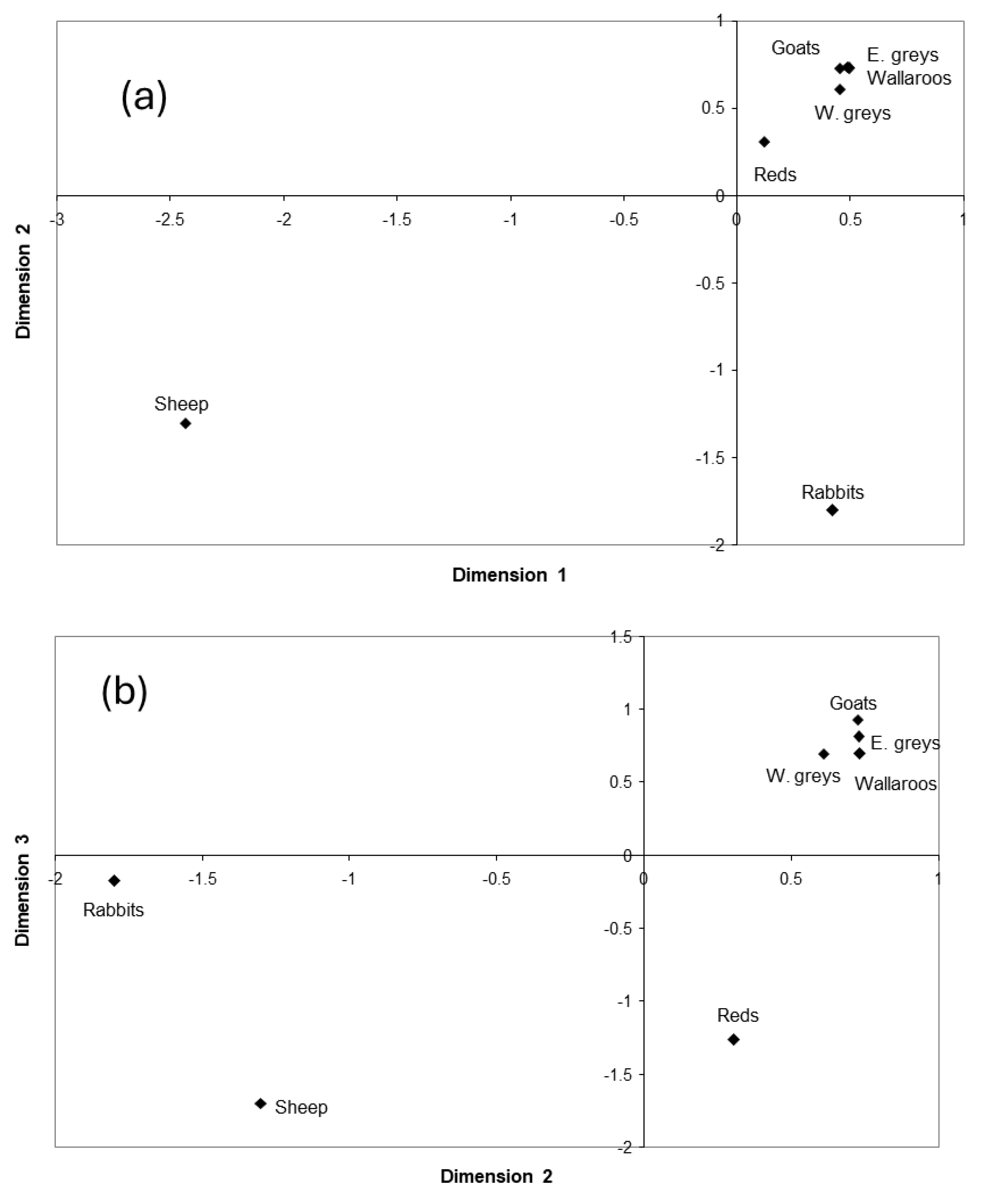
3.5.1. Multi-Dimensional Scaling

Multi-dimensional scaling (MDS) was applied to assess relative use of the study site by the herbivores. A dissimilarity matrix was constructed for each landclass (subject), based on ‘stimuli’ provided by the relative abundance of each herbivore species. The stimulus space provides points that correspond to each species. It presents information about how the entire group of subjects (landclasses) structures the stimuli. If the stimuli (species) are clumped near the origin, then these stimuli are not important on the dimension and not considered different from each other [68]. If the stimuli are at opposing ends of an axis representing a dimension, then that means they are both important and different from each other in that dimension. The subject space corresponds to vectors for each landclass. The direction of each subject (landclass) vector indicates the relative importance of each dimension to the subject and the vector length is proportional to the amount of variance in the subject’s data that is accounted for by the model [69]. Hence, vectors lying close to an axis are interpreted as important contributors defining the structure of stimuli (the herbivore species) in that subject. Both stimulus and subject space can be multi-dimensional. In this analysis, two- and three-dimensional models were constructed. The total amount of variance in the data set explained by the model is the RSQ value, and the stress factor is a measure of the proportion of error in the data that was created by the model. A small stress value and large RSQ value imply a good model.

Three-dimensional models generally produced better results. However, if the improvement over a two-dimensional model was marginal then the latter was used, as it is easier to comprehend. Separate analyses were conducted for stocked and unstocked paddocks to allow for the exclusion of sheep.

Unstocked Paddocks

Red kangaroos were the most abundant species, and rabbits were the most sedentary in the unstocked paddocks. They were clearly separated from each other and from goats, common wallaroos and eastern and western grey kangaroos in their relative abundance in landclasses (Figure 12). The remaining species clumped together nearer the origin than red kangaroos and rabbits. The examination of dimension 3 provided no further separation of species and maintained the relative relationships. Grey kangaroos, common wallaroos and goats were generally much less abundant, and their numbers not only fluctuated over time but their distribution over the landclasses varied to such an extent that large numbers of zeros were produced within the subject matrices. The closeness of the points representing these species in space, therefore, should not be confused with the apparent similarity between them and probably does not bear a realistic ecological basis. The MDS technique appears somewhat limited in separating species of low and fluctuating abundance on fewer landclasses than the more widespread red kangaroos and rabbits.

Red kangaroos were weighted most heavily in dimension 1 (D1), and responded strongly, but to a lesser extent, in dimension 2 (D2). Rabbits were clearly weighted heavily in D2 but not in D1. The weighting in D2 for both species indicates potential overlap.

Stocked Paddocks

The stimulus space in the stocked paddocks shows a clear separation of sheep from the other species along dimension 1 (D1) and rabbits from other species along dimension 2 (D2) (Figure 13a). Common wallaroos, eastern and western grey kangaroos and goats clump together in the unstocked paddocks, and the position of red kangaroos is poorly resolved in both of the first two dimensions. Red kangaroos segregate along dimension 3 (D3), and the differences between sheep, rabbits, red kangaroos and the remaining species are most clearly seen in the D2/D3 space (Figure 13b). Western greys also slightly diverge from common wallaroos, goats and eastern greys.

The results of MDS support the conclusions from the selection ratios and clearly show that sheep, rabbits and red kangaroos use the landclasses in quite dissimilar ways. The behaviour of the remaining kangaroo species and goats is less well resolved but differs from the three dominant species.

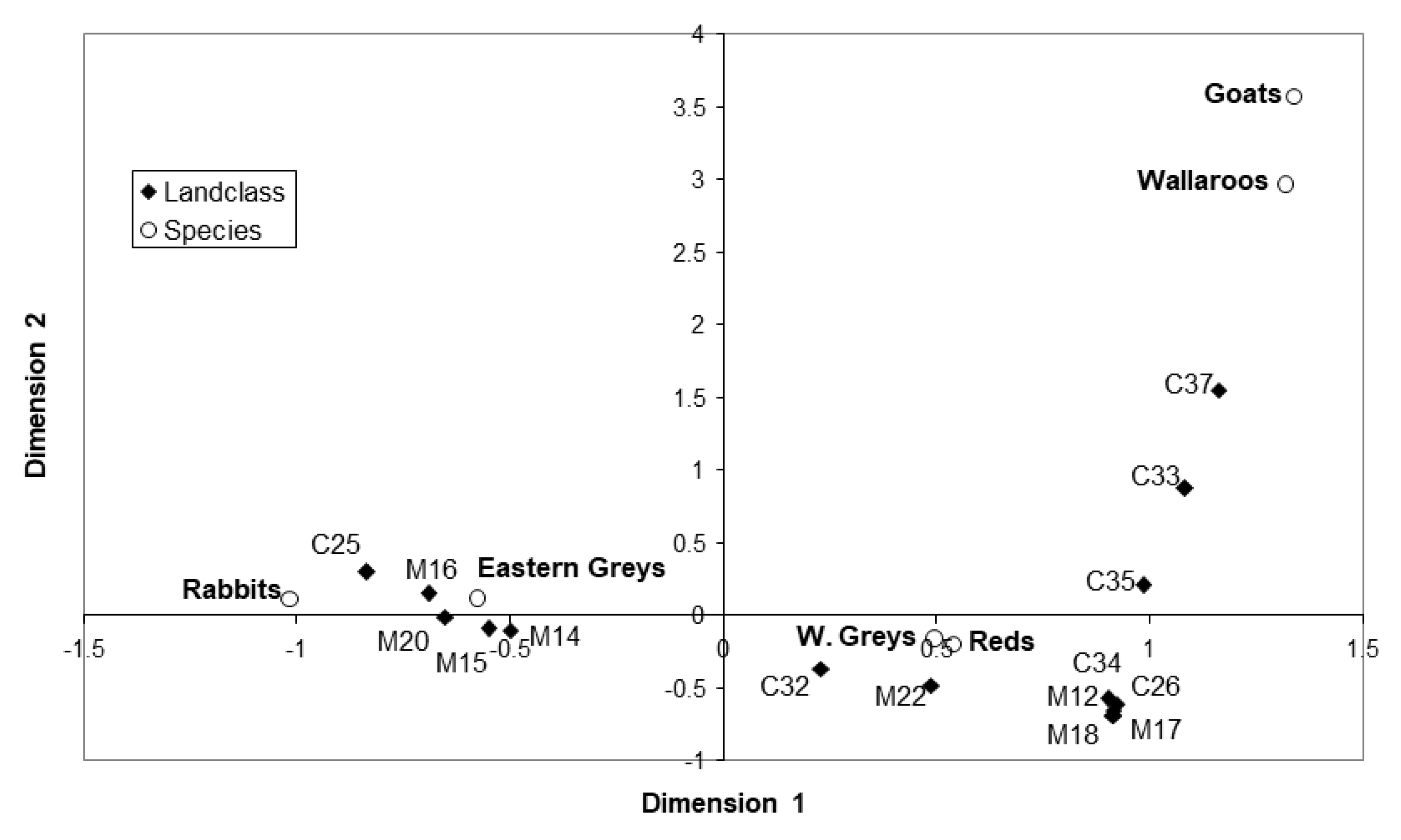
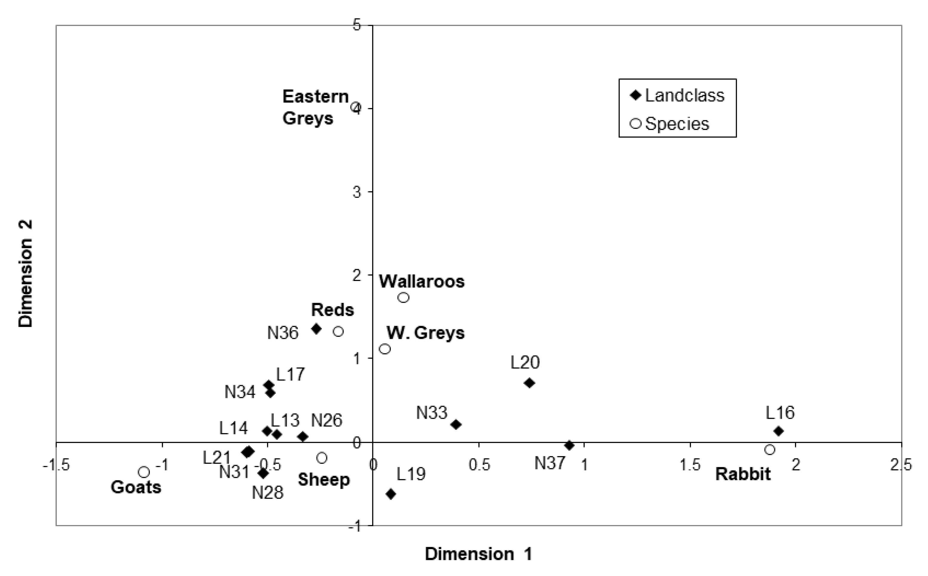
3.5.2. Correspondence Analysis

Correspondence analysis provided a better resolution of the relationships of all species, including the less abundant ones, than MDS. The habitat was again divided into stocked and unstocked paddocks for separate analyses.

In the unstocked paddocks, eastern grey kangaroos were most associated with the landclasses closest to Fowlers Gap Creek within Unstocked 1 and Unstocked 2 (Figure 14), as expected from the PUDs (Figure 11). Common wallaroos are also clearly segregated, suggesting a large degree of dissimilarity of habitat use over time when compared with all other species except goats, which shared the higher elevations. Common wallaroos were most closely related to the landclasses representing the foot slope and hill habitat, including drainage channels in Unstocked 1 (C33, C35, C37). Goats are the most distant species from any other, and this dissimilarity probably relates to their rarity and transience. However, the CA still placed them in the same structural space as common wallaroos, and indeed their rare sightings coincided with movement along the higher elevations of Unstocked 1, represented by C33, C35 and C37. This placement provides a greater level of confidence in this analysis than MDS. Western grey kangaroos were also relatively rare in the unstocked paddocks. However, they were placed close to red kangaroos, indicating strong similarities and hence some overlap in habitat use. When they were present, they were found in the same landclasses (C32 and M22) as red kangaroos. Red kangaroos were mostly associated with landclasses in the topographically lower parts of Unstocked 1 and the parts of Unstocked 2 with smaller clay pan areas (M12, M17, M18, M22, C26, C32 and C34). Rabbit abundance, in concert with the MDS analysis, was related to C25, M16 and M20, and landclass usage was dissimilar to other species.

In the stocked paddocks, the most distant species in the 2-dimensional space were eastern grey kangaroos, indicating a large dissimilarity likely based on their rare occurrence in these paddocks (Figure 15). Common wallaroos disassociated with goats and lie closer to red kangaroos and western greys, but they were never seen in Stocked 2, so the analysis is skewed by this absence. Despite these limitations, both species clustered in a more similar structural space to the red and western grey kangaroos than to the non-native domestic and feral herbivores, suggesting a closer association with their native relatives rather than with the introduced species. Red kangaroos were separated out along the negative direction of D1, opposing the placement of western grey kangaroos along that dimension, suggesting a degree of dissimilarity. However, both scale similarly along D2, indicating a degree of overlap as well. The landclasses most closely associated with red kangaroos are the ones located at lower elevations in Stocked 1 (N36, N34) and Stocked 2 (L17). Sheep are clearly separated from all other species in space and associated with a cluster of landclasses in Stocked 1 (N26, N28, N31) and Stocked 2 (L13, L14, L19, L21). They oppose all the kangaroos in the correspondence space, and hence, a clear segregation of the two taxa is evident. Rabbits occupy a different structural space from that of all other species. They scaled most closely to L16, an area of drainage channels with a suitable soil type for warren building. Goats also segregate from other species but are most similar to sheep.

Both MDS and CA show a clear separation of the most abundant and residential species. CA also established large dissimilarities between the less abundant and more transient species and clear differences between those and the abundant species. Both analyses established a relatively clear partitioning of habitat, so the same habitat is rarely used equally by two or more species at the same time.

3.6. Overlap in Habitat Usage by Herbivores

3.6.1. Species Richness

Species richness maps were constructed from each monthly population survey to determine multiple-use parts of the study site in a manner similar to analyses of biological diversity [70,71]. The observed pattern of richness agreed with a random model in only 6 out of the 33 monthly surveys analyzed. In the remaining 27 surveys, there were significantly more hectare blocks with one species than expected if the species were distributed in the study site at random.

The maximum richness was 2.5 species per hectare block (mean of two surveys) from a possible six species, as rabbits were not included in this analysis. There were relatively few blocks that had a maximum of more than one species (Figure 16a). The analysis of minimum richness determined that there was no block that was occupied in all surveys by one or more species. The average richness across all surveys did not exceed 0.5 species per hectare block (Figure 16b). This indicates a predominance of only one species present (values based on the mean of two surveys each month) at any one time in any block and hence strong species segregation at spatial and temporal levels.

The blank areas in these maps show some regions used by no species (Figure 16a) or very infrequently by any species (Figure 16b). In Unstocked 1, the no-use or low-use area coincided with large clay pans, and in Stocked 1, it coincided with the major drainage channel. In Stocked 2, an area dominated by woollybutt (an unpalatable grass) in the northern part of the paddock was infrequently used. Unstocked 2 was little used along the northern fence that coincided with erosion channels and clay pans.

Average richness per survey was not significantly correlated with herbivore density standardized as metabolic biomass (see [13] for conversion factors) (Spearman rank correlation, r_s = −0.46, p = 0.807). Thus, there was no evidence for increased overlap between species at times of higher herbivore load in the study site.

3.6.2. Overlap of Core Ranges of Herbivore Species

The population utilization distributions (PUDs) integrate each species’ common habitat usage over a longer time than the maps of richness. The locations for the more abundant species in the study site (viz red and western grey kangaroos, common wallaroos, sheep and rabbits) were divided into three 12-month periods, of which the first corresponded to drought. The total and core range of the population were calculated, but only the latter results are presented here. The overlap of core areas between species within each paddock was then calculated.

The populations of red kangaroos and sheep in the two stocked paddocks had minimal overlap in their core areas for the first year (

Table 7. Percent overlap of core area (MAP(50)) of herbivore populations in the study site during Years 1, 2 and 3 (1st value, 2nd value, 3rd value). ≥25% presented in bold; italics indicate that only few or no individuals were encountered in paddocks.

P		Red	W Grey	Wallaroo	Rabbit	Sheep
S2	Red		30.1, 36.8, 28.7		0, 1.1, 0	0.7, 12.6, 19.0
	W grey	31.1, 23.2, 45.5			0, 2.9, 0	1.5, 21.0, 27.3
	Wallaroo
	Rabbit	0, 16.7, 0	0, 6.7, 0			37.5, 33.3, 62.5
	Sheep	2.9, 10.9, 29.2	5.9, 26.6, 26.5		8.8, 1.8, 4.4
S1	Red		28.2, 14.3, 22.0	28.9, 7.7, 8.5	1.4, 2.4, 4.3	0.7, 11.3, 12.1
	W grey	49.4, 49.0, 56.4		14.8, 0, 3.6	0, 0, 0	12.3, 36.7, 41.8
	Wallaroo	36.3, 14.3, 38.7	10.6, 0, 6.5			0, 12.1, 16.1
	Rabbit	6.1, 16.7, 20.0	0, 0, 0	15.2, 20.8, 13.3	4.4, 5.5, 12.9	0, 12.5, 36.7
	Sheep	1.6, 17.8, 10.5	15.6, 16.8, 14.2	0, 10.3, 3.1	0, 2.8, 6.8
U2	Red		35.9, 13.2, 33.0	6.8, 8.8, 10.3	1.0, 0, 0
	W grey	48.7, 21.7, 49.2		17.1, 39.1, 13.8	3.9, 0, 1.5
	Wallaroo	53.8, 22.7, 50.0	100, 61.4, 45.0		0, 0, 0
	Rabbit	12.5, 0, 0	37.5, 0, 14.3	0, 0, 0
U1	Red		3.5, 18.9, 13.9	4.9, 0, 16.8	1.4, 0.8, 0.7
	Wallaroo	45.5, 38.5, 35.2		0, 0, 0	0, 1.5, 0
	Euro	15.9, 0, 31.9	0, 0, 0		15.9, 12.1, 6.9
	Rabbit	9.1, 6.3, 6.3	0, 6.3, 0	31.8, 25.0, 31.3

P = Paddock, U1 = Unstocked 1, S1= Stocked 1, U2 = Unstocked 2, S2 = Stocked 2.

). Overlap was greater in the two subsequent years but did not exceed 25% of the core area of red kangaroos. Red kangaroos consistently shared more than 25% of their core area with western grey kangaroos in Stocked 2. This pattern was repeated in Stocked 1 and Unstocked 2 in some years, consistently in the drought (Year 1), but not in Unstocked 1, where western grey kangaroos were uncommon. Red kangaroos had minimal overlap of their core area with common wallaroos and rabbits but once exceeded 25% with common wallaroos in Year 1 in Stocked 1.

Western grey kangaroos shared large proportions of their core population ranges with red kangaroos in all paddocks even though the common area was a much smaller proportion of the core ranges of red kangaroos. Likewise in the stocked paddocks, their core range had a high overlap with sheep but less so in the drought (Year 1). Western grey kangaroos had minimal overlap with common wallaroos and rabbits. The exception was with common wallaroos for Year 2 in Unstocked 2, where neither species was abundant.

The few common wallaroos that ventured into Unstocked 2 on the flood plains occupied areas that strongly overlapped with the abundant red kangaroos and the few western grey kangaroos in this paddock. In the slope paddocks, Unstocked 1 and Stocked 1, the overlap of core population ranges was the strongest with red kangaroos. The overlap with western grey kangaroos, rabbits and sheep was relatively small in these slope paddocks.

In contrast, there was a high overlap of the core population range of rabbits with common wallaroos in Unstocked 1 and, to a lesser extent, in Stocked 1. The overlap of the core area of rabbits was minimal for the other species in both slope and plains paddocks.

The core population range of sheep in Stocked 1 included little of that of the other species. In Stocked 2, the overlap was greater with western grey and red kangaroos except during the drought (Year 1).

These patterns of overlap are consistent with the relative segregation of sheep and rabbits from the kangaroo species in the previous analyses of habitat usage.

3.7. Spatio-Temporal Habitat Use of Individual Radio-Tracked Herbivores

3.7.1. Home Range Estimates, Locations and Movement of Kangaroos

Eastern Grey Kangaroos

The radio-tracking of the five eastern grey kangaroo females confirmed that they rarely entered the study site (see Figure 11a). Rather, they confined their movements to the habitat in and adjacent to Fowlers Creek (Figure 17).

Eastern grey kangaroo home ranges were small: MAP(50) = 23.3 ± 3.7 ha, MAP(95) = 94.9 ± 22.3 ha (n = 5). Only 5.5% of locations were within the study site. On these rare occasions, only unstocked paddocks were visited. Both these paddocks shared a fence line with Saloon paddock, the paddock that encompassed Fowlers Greek. Thus, the radio-tracking confirmed the results of the population surveys that showed eastern grey kangaroos were a minor and transient component of the herbivores in the study site.

Red Kangaroos

From the 34 red kangaroo females that were radio-collared over the first two years of the study, three individuals were rejected from the sample because they were tracked only for very brief periods (<5 months) before they died. One was rejected because it moved off the study site shortly after capture and remained off the site. This reduced the sample to 30 individuals that were tracked for a minimum of 8 months and a maximum of 33 months.

The total sample of locations was used to calculate one estimate of the MAP(50) and MAP(95) ranges for each individual. Six red kangaroo females (and six western grey kangaroo females) were tracked for more than two years when they experienced both prolonged sparse and good pasture conditions relating to rain. Their locations were divided into two subsets, ‘drought’ and ‘normal’, and MAP(50) and MAP(95) ranges were estimated separately for each period.

The red kangaroo females in the study site occupied on average a core area (MAP(50)) of 84.0 ± 10.2 ha and a total home range ((MAP(95)) area of 318.7 ± 33.1 ha (n = 30). There were no significant differences in home range size between individuals tracked for more than two years when compared to those tracked for less than two years. Thus, sample sizes appeared adequate to define the general extent of an individual female’s movements.

Core (drought = 57.5 ± 15.0 ha; normal = 50.2 ± 8.3 ha) and total home range sizes (drought = 234.9 ± 55.5 ha; normal = 227.1 ± 36.9 ha) did not differ significantly between the drought and more normal conditions. (Wilcoxon signed-ranks test, p > 0.05, n = 6). Three individuals expanded and three individuals contracted their home range during drought. Thus, individuals did not significantly expand their foraging radius during periods of nutritional stress. However, home ranges shifted slightly. The overlap between the drought home ranges relative to the home ranges occupied during normal conditions ranged between 35.5% and 93.9% for the core areas (mean ± SE = 56.1 ± 9.1%) and between 23.0% and 81.7% for the MAP(95) home ranges (mean ± SE = 62.9 ± 9.6%).

Eighteen of the red kangaroo females were commonly found in the unstocked paddocks (Figure 18). These females remained within the unstocked paddock boundaries for most of their tracking period. Those females mostly associated with the stocked paddocks (10 individuals) tended to incorporate parts of adjacent paddocks within their home ranges (Figure 19), spending considerable time in Unstocked 1, Unstocked 2, and two other adjacent paddocks. The home ranges of two individuals were equally spread over stocked and unstocked paddocks (Figure 20).

The core and total home range sizes of individuals located predominantly in stocked paddocks (n = 10) were significantly larger than those in unstocked (n = 18) paddocks (Mann–Whitney Test, MAP(50): Z = −2.255, n = 28, p < 0.05, MAP(95): Z = −2.446, n = 28, p < 0.05).

Western Grey Kangaroo Females

Six western grey kangaroo females were rejected from the sample of fifteen that were radio-collared because they either spent their entire time (except drinking) outside the study area or were tracked for too short a time to generate reliable results. Three females were lost to choroid retinitis disease (Kangaroo blindness [72]). The reduced sample of nine females was tracked for between 12 and 34 months.

Western grey kangaroo females occupied an average core area of 57.8 ± 4.6 ha and home range area of 196.9 ± 15.9 ha (n = 9). Neither the size of the core nor home range area of the western grey kangaroo females was significantly different from those of red kangaroo females. Western grey kangaroo females’ home ranges were in Unstocked 2, Stocked 1 and Stocked 2 about equally (Figure 21). Only three of the western grey kangaroo females were predominantly located in an unstocked paddock, so comparisons with respect to home range size between stocked and unstocked paddocks could not be statistically evaluated.

Six western grey kangaroo females were tracked for sufficient time to evaluate home range size during ‘drought’ and ‘normal’ conditions. Like red kangaroos, the sizes of core areas (drought = 49.1 ± 10.4 ha; normal = 54.6 ± 4.3 ha) and home ranges (drought = 157.9 ± 34.1 ha; normal = 197.1 ± 18.4 ha) did not significantly differ. However, the statistical power of a sample of six is relatively weak, and in fact, five out of six females showed a slight contraction in the total (MAP(95)) home range size during drought.

The home ranges of western grey kangaroo females in the stocked paddocks were significantly smaller than those of the red kangaroo females (Mann–Whitney Test, n₁ = 6, n₂ = 18, MAP(50): Z = −2.490, p < 0.05; MAP(95): Z = −3.467, p << 0.001).

3.7.2. Mobility of Red and Western Grey Kangaroos

The weekly tracking of each individual female provided a chronicle of her movements over time and in space. Strong site fidelity was demonstrated in red and western grey kangaroos. However, 5 of the 54 individuals (4 red kangaroos, 1 western grey kangaroo) were lost. These females probably moved a significant distance and out of range of the receiver. Regular grid searches for dead kangaroos were conducted in the study site but did not uncover their corpses in any of the four paddocks. Thus, 9% of the radio-tracked females (12% of the red kangaroos, 7% of the western grey kangaroos) were either transient non-residents in the study site or emigrated. The remaining 91% (88% of the red kangaroos, 93% of the western grey kangaroos) were sedentary, implying that most mature females in the studied population behaved likewise.

Even so, movements of several kilometres did occur, particularly amongst the red kangaroo females. The movements were likely in response to a changing resource base. The most significant occurred around a high rainfall event at survey 11 (see Figure 1). Red kangaroo females tracked at that time shifted from their usual core area (Figure 22). The maximum distance detected was 5.85 km (n = 16). By comparison, the maximum distance detected for western grey kangaroo females was 1.52 km (n = 8). There was a significant difference between the species in the maximum distances travelled (Mann–Whitney Test, Z = −2.082, p < 0.05). These movements occurred along a northeast/southwest-orientated corridor traversing the study site and intruding onto one of the neighbouring pastoral properties (Sturts Meadows) to the south. Some individuals remained in their new location for several weeks before they returned to their place of origin. Four of the red kangaroo females disappeared completely out of sight and signal range after having moved off the study site for a period of about three to four weeks, indicating an even longer distance travelled than the maximum calculated above. However, all subsequently returned to the original core area of their home range, with one individual returning after 5 months.

The movement was in response to a relatively heavy rainfall of >25 mm at survey 10 that followed several months of drought and, consequently, very poor pasture conditions. High mortality of kangaroos was evident by the time of the rain event. This rain caused not only the greening of the perennial grasses but also the germination of annual grasses. The highest falls were in a corridor traversing the eastern side of Fowlers Gap Station, including the study site. Adjacent areas did not receive the same amount of rainfall or received it later (Figure 22). Hence, the vegetation did not respond equally in all areas.

Thus, as the perennial grasses greened quickly, the red kangaroos responded by moving to this resource. Subsequently, significant germination occurred and yielded a substantial biomass of fresh green annual grasses (mostly button grass, Dactyloctenium radulans) preferred by kangaroos. Annual vegetation was more common in the unstocked paddocks (and areas in other paddocks where there were few shrubs). These swards of fresh green grass attracted a large influx of individuals not usually resident on the site (see Figure 3). The movement of about 5 km undertaken by radio-collared individual females suggested movement of at least that scale from either side of the higher rainfall corridor. Since males and young animals tend to move even longer distances than mature females [73], this catchment could have been broader. However, as the females returned to their original home ranges in response to more widespread rainfall, the high densities of red kangaroos in the study site also decreased within a few weeks. This suggested a return of the temporary immigrants to their original home range as well.

Figure 22. Rainfall (mm) pattern between surveys 10 and 16 at four gauges: (a) northwest, (b) north, (c) in and (d) southwest of the study site and the movement of female red kangaroos along a north–south gradient in the same period. Each female is colour-coded and her core area in the study site is shown as a large polygon, and locations outside are indicated by the same colour circles. The arrow indicates the start of local rainfall. The peak in the study site is the third gauging. Coordinates are truncated from Australian Map Grid (65xxxxx north, 5xxxxx east). From [74] with permission.

Figure 22. Rainfall (mm) pattern between surveys 10 and 16 at four gauges: (a) northwest, (b) north, (c) in and (d) southwest of the study site and the movement of female red kangaroos along a north–south gradient in the same period. Each female is colour-coded and her core area in the study site is shown as a large polygon, and locations outside are indicated by the same colour circles. The arrow indicates the start of local rainfall. The peak in the study site is the third gauging. Coordinates are truncated from Australian Map Grid (65xxxxx north, 5xxxxx east). From [74] with permission.

Western grey kangaroo females did not significantly increase their mobility in relation to drought or a substantial decrease in pasture availability, unlike red kangaroos. There was no significant change in the density of western greys in response to patchy rainfall on or off the study site (Figure 6a). They remained largely within their normal home range throughout the events that precipitated long-distance excursions by many red kangaroos. The overlap of drought core areas with core areas in normal pasture conditions ranged from 25% to 84% (mean ± SE = 50 ± 9%) for the six western grey kangaroo females tracked long-term. Home range overlaps ranged from 43% to 73% (mean ± SE = 57 ± 5%). These values did not differ significantly from the overlap calculations for red kangaroo females since the long-range excursions for the latter were few and relatively brief.

3.7.3. Home Range Quality

Individual red and western grey kangaroo females were tracked for different time periods and during varying environmental conditions. To maximize the information available from each individual, home range qualities were assessed relative to those of the study site as a whole for those vegetation and population samples taken during the period an individual was radio-tracked. The mean value per hectare block was calculated for the study site (Ms) and the individual’s home range (Mi). The value for the individual was then expressed as the proportional difference to the mean of the study site ([Mi-Ms]/Ms). The ‘proportional difference’ may be positive, indicating more of a particular resource, or negative, indicating less of a particular resource available within the home range compared to the study site as a whole. A similar measure was derived for tree density and geographic features of the study site, which were assumed to remain unchanged across the study period.

Correlations were performed to determine whether any of the home range quality variables were significantly related to any other variable to assess problems of collinearity in multivariate statistical procedures. Measures of forb and grass biomass were significantly correlated to those of green forbs and green grasses, respectively. Thus, the proportional difference in green forbs and grasses was used since this reflected the kangaroos’ dietary preference. Slope and contours were also highly correlated, so only the variable ‘slope’ was used as it better reflected run-on/run-off zones. The final variable set included 13 proportional differences. Two red kangaroo females were rejected from the analyses because more than 50% of their home ranges fell outside the study area. Therefore, the final sample was reduced to 28 red kangaroo females and 9 western grey kangaroo females.

Discriminant Function Analysis (DFA) was applied to the MAP(50) areas. Some red kangaroo females (3 out of 28 analyzed) occupied core areas with habitat qualities like western grey kangaroo females, but more western grey kangaroo females (5 out of 9 analyzed) had core areas like red kangaroo females. The proportion of western grey kangaroos within the core area was the most discriminating variable separating the two kangaroo species (

Table 8. Discriminant Function Analysis—Variables (proportional differences) and mean scores for red and western grey kangaroo female core areas (MAP(50)). * significant differences between species using 1-way ANOVA. (FLC = flat-leafed chenopod shrub, RLC = round-leafed chenopod shrub).

Variable	Red Kangaroo	Western Grey Kangaroo
Red density	0.39	0.12
Western grey density *	0.24	2.02
Sheep density *	−0.22	0.82
Wallaroo density	−0.70	−0.83
Rabbit density	−0.45	−0.53
Copperburr biomass	0.06	−0.04
a Green forb biomass	−0.02	0.00
b Green grass biomass	−0.04	0.02
FLC biomass	−0.54	−0.49
RLC biomass	−0.04	0.11
Tree density	0.47	1.87
Slope	−0.49	−0.52
Water distance	−0.32	−0.39

^a expressed as proportion of total grass biomass. ^b expressed as proportion of total forb biomass.

). While the density of western grey kangaroos in the core area was more than 200% higher than in the study site as a whole for western grey kangaroo subjects, it was significantly less at about 25% higher for red kangaroo subjects (F_1,35 = 15.28, p << 0.001). Tree density within the core areas of red kangaroo subjects was only approximately 50% higher than on average over the study site but was almost 200% higher than the average in core areas of western grey kangaroo subjects (F_1,35 = 3.791, p = 0.06). Hence, the density of western grey kangaroos and the density of trees (overhead shelter) played a significant role in western grey kangaroo core areas, but less so for red kangaroo subjects. The density of sheep was below the average for the habitat within red kangaroo core areas (mean = −0.22) but a significantly higher than average density in western grey kangaroo core areas (mean = 0.82) (F_1,35 = 4.335, p < 0.05). This result concurs with that of the population distributions, where a closer association of sheep and western grey kangaroos was established than that shown by sheep and red kangaroos. Both kangaroo species had significantly less flat-leafed chenopod biomass and density of common wallaroos and rabbits within their core areas than were present on average across the study site. Likewise, there were negative relationships with slope and water distance.

The home range size of radio-collared females was regressed against key habitat variables that expressed little collinearity. The variable set included the proportional difference between the MAP(50) or MAP(95) area and the study site for the densities of red kangaroos, western grey kangaroos, sheep, rabbits and common wallaroos, the biomass of copperburrs and flat-leafed and round leafed chenopods, the proportion of green grass and green forb biomass (from the total grass or forb biomass, respectively), the distance to water and the slope. The slope variable tended to correlate with common wallaroo density and water distance variables, so analyses with and without this variable were conducted. The analyses were weighted by the proportion of each female’s home range contained within the study site. Two samples were used: one with red kangaroos (n = 28) and one with western grey kangaroos (n = 9).

No significant relationship was found between the MAP(95) area of western grey females and any of the home range quality variables. In contrast, the MAP(95) area of red kangaroo females increased linearly with a proportional increase in biomass of flat-leafed chenopods (mainly Bladder Saltbush—Atriplex vesicaria) (Beta = 0.750) and density of sheep (Beta = 0.291) (R² = 0.71; F_2,25 = 29.95, p << 0.001).

MAP(50) areas produced opposite relationships for western grey and red kangaroo females in relation to the proportional difference in flat-leafed chenopod biomass. The core area of western greys significantly decreased in size (Beta = −0.67) as the home range had relatively more biomass (R² = 0.45; F_1,7 = 5.62, p = 0.05). Moderate partial correlations were found with round-leafed chenopod biomass (−0.575) and tree density (0.354). A model with these variables explained more variance (R² = 0.65), but the relationship was not significant (F_3,5 = 3.123, p = 0.13). The core area of red kangaroos increased significantly (Beta = 0.836) as it contained proportionally more flat-leafed chenopod biomass (R² = 0.70; F_1,26= 60.35, p << 0.001). Partial correlations significant at the 10% level were found with red kangaroo (−0.345), sheep (0.336) and western grey kangaroo (0.364) densities. A model with western grey kangaroo density explained more variance (R² = 0.74) in a significant relationship (F_2,25 = 35.34, p << 0.001). Since western grey kangaroos have smaller core areas in ranges with more flat-leafed chenopod biomass, as expected, red kangaroos have larger core areas where western greys were denser.

3.7.4. Home Range Quality and Reproductive Success

Each home range quality variable for the core and total home range area was related to the reproductive success of radio-tracked female kangaroos. Reproductive success was measured as the weaning success of young-at-foot: either a weaning ratio, calculated by dividing actual weaning success by the number of weaning attempts possible during the tracking period, or a binary measure of weaning success (none = 0, some = 1). This required females to be tracked for at least a year for them to potentially wean at least one offspring. Red kangaroos can wean young within a year (8 months pouch life, 4 months to weaning), whereas western grey kangaroos have a longer pouch life (around 11 months) and up to 6 months to weaning. However, all females used in the analysis had young at a stage where they could bring one to weaning. This constraint reduced the sample to 33 females, 24 red and 9 western grey kangaroos.

The western grey kangaroos were significantly more successful in weaning their young (median = 0.67, n = 9) than red kangaroos (median = 0.13, n = 24) (Mann–Whitney, Z = −2.619, p < 0.05). However, there was no significant difference in the size of their core area (western greys, median = 64.0 ha; reds, median = 78.0 ha) nor any other single quality of the core area except the relative density of trees (Mann–Whitney Test, Z = −2.425, p < 0.05). For the latter, western grey kangaroo core areas had nearly double the average habitat density of trees (median proportional difference = 0.87), whereas those of red kangaroos were about average for the habitat (median = −0.06). Red kangaroo females occupied significantly larger home ranges (median area = 347 ha) than western greys (median = 198 ha) (Mann–Whitney, Z = −2.022, p < 0.05). Like the core areas, western greys occupied home ranges with relatively high tree densities (median proportional difference = 1.00), significantly greater than red kangaroos (median = 0.18) (Mann–Whitney, Z = −2.951, p < 0.01). Red and western grey kangaroo home ranges fell within similar densities of red kangaroos (median proportional differences = 0.25, 0.12, respectively) but significantly different densities of western greys (median proportional difference = 0.21, 1.03, respectively) (Mann–Whitney, Z = −2.223, p < 0.05).

No single home range quality variable or combination for the core area explained a significant amount of the variation in the weaning ratio of red and western grey kangaroo females. Multiple regression models only found a significant effect of species, confirming the univariate tests presented above. Similar models, including species as a dummy variable for the home range, revealed a weak inverse relationship between the home range size and weaning ratio for both species combined (R² = 0.24, F_1,31 = 10.03, p = 0.003). However, separating the results of the two species suggested the relationship only held for red kangaroos.

Many red kangaroo females weaned no offspring, so the core and home range sizes and qualities of those with no success and some success were compared with a series of univariate tests. These tests included an additional measure of the proportion of drought months included in their tracking period. No significant difference between these groups was found.

Moss [75] found that the age of the female, rather than home range size, best explained reproductive success in his study. Female red kangaroos older than 10 years were significantly more successful. No such difference was found here for the weaning ratio (<10 y: mean = 0.24 ± 0.08, n = 14; ≥10 y: mean = 0.34 ± 0.13, n = 10) (Mann–Whitney U, Z = 0.49, p = 0.7). The two age groups did not differ significantly in the size or relative quality of their home range or core area. The sample size of western grey kangaroo females was insufficient to warrant a similar statistical analysis.

Relationships with habitat quality were strengthened in red kangaroo females by the reduction in the variable set to a smaller orthogonal set of factors (Appendix D) and then performing multiple regressions with them. The final model included scores on Factors 3 and 2, where Factor 3 principally related to high relative tree density and Factor 2 related to high densities of sheep and western grey kangaroos and a low density of red kangaroos and a low biomass of copperburrs (R² = 0.0.49, F_3,20 = 6.38, p = 0.003). Since the standardized coefficients were all negative (home range size = −0.828, Factor 3 = −0.609, Factor 2 = −0.37), the conclusion is that higher weaning success is found in red kangaroo females with relatively small home ranges in areas of low tree, sheep and western grey kangaroo density with more of their own species and a higher biomass of copperburrs.

4. Discussion

4.1. Population Dynamics

The dynamics of the kangaroo populations were controlled predominantly by rainfall conditions and pasture availability. They therefore do not differ from populations elsewhere in the region (e.g., [27,76,77]). Changes in density were due to variation in reproductive success and mortality, immigration and emigration, with different weightings of these factors for species in the study site according to where the source population typically resided. These factors were closely related to food quantity and quality. Previous studies of red kangaroos have drawn similar conclusions that the density and distribution of populations are due to localized responses of these herbivores to the distribution of desirable pasture [78,79,80,81], water resources and possibly shelter. Furthermore, studies on populations of red kangaroos, western grey kangaroos and common wallaroos in the region and elsewhere have found that densities were constrained primarily by food availability, especially in the absence of predation and lethal control [24,27,82,83,84,85,86].

Although food availability is the proximate factor, rainfall is the ultimate influence, governing both the growth or decline of plants and the increase or decrease in the animals grazing on them. Rainfall in the arid zone, however, is erratic and unpredictable, and temperatures vary over a wide range. This, in turn, leads to equally unpredictable vegetation dynamics in terms of the quantity and quality of pasture plants [13]. The herbivores attempt to track these changes in the resource base with some lag, with a resultant change in their population size and composition.

Unlike the unmanaged kangaroo species, the other three herbivores were subject to human interventions. Goats were mustered four times during the study period, and around 450 were removed to market. The management of sheep numbers was a function of climate and market factors. Lambs were removed after weaning, and stocking rates were adjusted annually post-shearing in November, according to an assessment of vegetation resources per paddock and recommended stocking rates. Rabbits were initially controlled by the frequent release of the myxomatosis virus and a single release of calci-virus towards the end of the study. Rabbits also had mortality from the collapse of warrens in clay soils along drainage channels after rare heavy rainfall.

The population of the most abundant species, the red kangaroo, fluctuated in response to variable rainfall conditions and subsequent changes in pasture biomass, as was expected. Red kangaroo numbers also declined slightly over the study period, indicating mortality due to drought in the first year and slow recruitment following improvement in pasture availability towards the end of the study. The density of red kangaroos was typically 0.25 individuals ha⁻¹. Red kangaroos are predominantly active at night [51]. Night counts significantly correlated with day counts, so their populations were accurately assessed during the early morning when visibility is better than at night.

A patchily distributed rainfall event of more than 50 mm interrupted a lengthy period of otherwise severe rainfall deficiency. The red kangaroo population peaked in all paddocks, reaching a density ten times higher than average in the unstocked paddocks and two to three times higher in the stocked paddocks. The precipitation led to a flush of green pasture, particularly summer grasses, in the study area and along a gradient traversing the property in a northeast/southwesterly direction that included the study site. Outside this gradient, the greening of pasture was delayed, leading to the immigration of many individuals from surrounding paddocks and possibly even surrounding pastoral properties into the rainfall-affected area. The ‘immigration’ event was transient and lasted only a few weeks, after which the kangaroos dispersed again. Croft [32] described the movement of some radio-collared red kangaroos in Fowlers Gap in a similar event. Edwards et al. [73] tracked a similar large transient increase in the population density of red kangaroos, where, after a dry period of six months, a local rain shower stimulated ‘green pick’, which, although scant, attracted large numbers of red kangaroos into their study site. Red kangaroos are mobile and hence able to distribute themselves over their range in response to various stimuli [80], of which the availability of freshly germinating grasses ranks highly due to their diet preferences [22].

At the time of the influx of red kangaroos into the study site, individuals tagged with radio-transmitters and usually counted as residents, also moved several kilometres up or down along the gradient of higher precipitation. However, most returned to the core of their original home range area within a month or two. Thus, it is likely that the excess individuals immigrating into the study site returned to their place of origin when pre-influx densities were attained once again. Hence, permanent recruitment did not occur. This concurs with prior studies [32,34] that concluded that red kangaroos are not typically nomadic but may move up to 50 km due to localized rainfalls during drought. Furthermore, they have a demonstrated homing ability [32,33] and are capable of returning to their original home range once widespread rainfall breaks drought conditions. Even so, some tagged individuals, usually males, have been located 100 or more kilometres from the point of capture [43]. Fidelity to a home range is not inclusive of all age/sex classes. The populations of the other unconstrained herbivore species did not follow the trajectory of the red kangaroos and remained relatively stable throughout the rainfall event.

Previous studies of the population dynamics of red kangaroos have counted individuals at 3-month intervals at scales ranging from paddocks [75,87] to pastoral leases [27], and annually in winter in pastoral zones [88] or large management areas [89]. A shorter monthly interval proved effective in unravelling the conditions behind mass changes in the population. Such high influxes of red kangaroos are unlikely to be a long-lasting burden on vegetation resources, as they are as transient as the pasture response. However, land managers often argue for damage mitigation when large numbers of kangaroos invade their properties, since they assume any bounty they gain from localized rainfall is lost to the invaders [90]. The impact is likely to be short-term as the events are too stochastic to expect repeated grazing down of an area. The resource is superabundant relative to the herbivore densities and rapidly dies off without follow-up rain. Observations of captive and free-ranging red kangaroos show they are very sensitive to a reduction in pasture due to the energetic costs of intraspecific (and perhaps interspecific) competition for resources [25,91]. Thus, they are likely to avoid a situation where it becomes energetically too expensive to find food due to depletion by too many competitors. Rather, they move out of such an area in search of a better pay-off elsewhere. Their strong home range fidelity implies that this is most likely to be to their original range and a familiar environment after general rainfall, instead of venturing on again into the unknown.

The greatest influx of red kangaroos was into the unstocked paddocks with their already higher population, indicating a faster response of vegetation in these paddocks, possible avoidance of sheep or a combination of these factors. Conversely, the subsequent drop in densities following the short-term increase could, of course, be interpreted as a response to a decline in pasture conditions following high grazing pressure. This would be a density-dependent response. But density-dependence requires an increase in birth rates under low-density conditions to reach an equilibrium point. There was no evidence for this during this study, as the proportion of adult females with young-at-foot reflected pasture conditions, not population size. The per capita growth rate of the population did not depend on its own density. Likewise, at higher densities, mortality should increase if the population was density-dependent, but again, mortality was a response to low pasture biomass. Hence, the population dynamics in the study site appear to be density-independent, and the availability of food controls red kangaroo abundance.

Red kangaroo densities were significantly higher in the paddocks without sheep. The two paddocks, Unstocked 1 and Unstocked 2, were taken out of the sheep-grazing regime about 30 and 10 years, respectively, prior to this study. In both cases, the purpose was for research either on the recovery of severely degraded land (Unstocked 1) or examination of red kangaroo-sheep competition (Unstocked 2 was destocked since it was judged of little value to sheep production). The stocked paddocks have been assessed as being favourable to sheep production since they retained a good cover of chenopod shrubs (especially bladder saltbush) as a drought reserve. However, the densities of red kangaroos in these paddocks were not only consistently lower but also more variable. The abundance of red kangaroos in stocked paddocks tended to equal that of sheep but decreased significantly at lamb dropping time. This coincided with ewes separating from the flock to give birth and to bond with their lambs before forming a cohesive flock again. With flock cohesion, kangaroo densities increased slightly again but remained below initial levels until after shearing time. The latter also coincided with the separation of lambs from ewes and therefore with a lower density of sheep again. The difference in densities and the drop in numbers when lambs were present in the paddocks is evidence of avoidance (interference competition) of widely dispersed sheep. A shift in habitat preference due to a coincidental change in pasture conditions or shelter needs cannot be dismissed but is unlikely [13]. Obviously, more lambing events in stocked paddocks need to be observed, and more replicates of unstocked paddocks without confounding habitat differences need to be investigated. Stocking treatments could also be reversed to see whether the red kangaroo population switches its preference.

The red kangaroo population in the study site was typically female-biased, like other studies [92,93]. However, the actual proportion of adult females varied with pasture condition. The population initially had a high proportion of young-at-foot and juveniles that were mostly lost in the subsequent drought, when adult females dominated at around 70% of the population. Drought is understood to bias the sex ratio towards females by truncating age structures [88]. The youngest members of the population are typically the most vulnerable during times of severe resource stress, as experienced in a drought. Juveniles suffer from digestive constraints [94] that require a relatively high-quality diet of sufficient quantity. Young animals do not have sufficient body reserves to cope with the nutritional stress of drought, causing them to quickly lose condition and die [6,95]. Skulls of young kangaroos were difficult to find as they were consumed or buried by foxes and taken to the nests of eagles. We therefore inferred high juvenile mortality through the drought from the large decline in the proportion of adult females with young-at-foot and juveniles as a proportion of the population. McLeod’s [96] research on the same study site predicted that males larger than 50 kg would find insufficient herbage to fill their large guts and would perish from starvation in drought at a faster rate than smaller males and females. We confirmed this prediction since adult males were at their lowest proportions in the population during the drought. The highest relative mortality was in the >12 y age classes of both sexes, but the drought cut into all age classes. Adult males suffered similar mortality in both drought and good conditions, but at a higher rate in the drought when their population was also much higher. The ageing of skulls taken from individuals that died during the study revealed the expected mortality of old individuals of both sexes. The mortality rate was significantly accelerated by the drought. Old individuals may have extreme tooth wear and other age-related disabilities not allowing them to chew and digest the remaining tough vegetation during dry times, leading to poor body condition and subsequent death [86]. Unexpectedly, many mid-aged (around 8-year-old) individuals also died. Robertson [97] calculated the age structure of dead red kangaroos during prolonged drought in Kinchega National Park (also in western New South Wales). The highest survivorship was found in the age group of 3- to 8-year-old individuals, an age range that falls within the optimal body weight range established by McLeod [96].

The reproductive success of red kangaroos was the highest at the start of the study and increased again towards the end. However, the proportion of females seen with dependent young was lower than expected and indicated a high mortality of young-at-foot, even under average conditions. The reproductive success of females in stocked and unstocked paddocks did not significantly differ. Thus, any competitive effect of sheep on red kangaroos was not expressed through impaired reproduction to the young-at-foot stage. Edwards et al. [23] likewise found an impact of sheep on the body condition of red kangaroos during a very dry period but none on reproductive success. Both western grey kangaroos and sheep had higher reproductive success, with sheep ranked first. We did not separate the effects of kangaroos on sheep, as all species were free to roam in stocked paddocks. However, Edwards et al. [23] found only a depression of liveweight of sheep but not reproductive success when a kangaroo effect was experimentally tested.

The less abundant western grey kangaroos significantly increased their population over the study. In Stocked 2, variation in their population significantly positively correlated with that of sheep. Western grey kangaroos prefer habitats with some dense lateral cover [81], which was better met in the stocked paddocks that had denser stands of prickly wattle (Acacia victoriae) and more shrub cover [13]. The western grey kangaroos suffered comparable mortality in the ‘drought’ to red kangaroos (22%), contrary to Robertson’s [97] finding of a much higher drought mortality at Kinchega National Park. An outbreak of the choroid retinitis disease during the second two years of the study led to higher mortality in western grey than red kangaroos [98], but neither event curbed their population growth. The likely explanation is that reproductive success was sustained and higher in western grey than red kangaroos, even though the latter has a higher reproductive rate. Pouch life in western greys is 323 days, almost the time when young red kangaroos reach weaning. Weaning in western grey kangaroos occurs after 540 days. Western grey kangaroos lack embryonic diapause [99], so each offspring is a greater proportion of their reproductive potential than for red kangaroos. Thus, whereas the drought suppressed the red kangaroo population’s reproductive success, it may not have been hard or long enough to cause a significant decline in the reproductive success of the western grey kangaroos.

Barker [100] summarized dietary studies in western New South Wales and southern Queensland that showed that western grey kangaroos were more generalist foragers during dry times than red kangaroos. They readily utilized shrubs and even trees during pasture shortage, forage that was readily available in the stocked paddocks through the drought. In contrast, red kangaroos, even in poor times, select for grasses [22,100] that were significantly depleted in drought. This forage selection might have given the western grey kangaroos the edge at the time of this study. However, the reproductive and foraging strategies of both species are likely to have advantages and disadvantages, and success might be balanced after a run of good years. There was no evidence that populations of either species influenced the other, except in Unstocked 2, where the correlation was negative. This was the paddock that sustained the highest densities of red kangaroos on the most ephemeral pasture [13], and this is where this species might be most advantaged relative to its congener.

Eastern grey kangaroos were rare in the study site, and their occurrences coincided with winter periods and times of poor pasture. These movements appeared to be independent of the variation in the populations of any of the other kangaroo species, goats or rabbits. Eastern grey kangaroos are relatively poorly adapted to the extreme heat stress, limited tree cover and sparse grass cover of the arid zone [101,102]. The population of eastern grey kangaroos in Fowlers Gap was mostly associated with riparian vegetation along the major creek lines, such as Fowlers Creek. Although the population was centred off the study site, radio-tracking of a small cohort of females suggested that the population did not obviously increase or decline.

Common wallaroos were at higher densities in the slope paddocks due to their selection of slope and ridge habitat [37]. Peaks in density coincided with autumn when summer-growing grasses tend to be depleted [13]. Common wallaroos show a strong preference for grasses and attempt to remain on this diet as long as possible [103]. Most individuals were medium- and large-sized males. These have higher absolute energy requirements than smaller individuals of the same species, needing substantially more bulk to maintain their body weight. Hence, they move to a better quality habitat. Due to their size, they are also less likely to fear predators, unlike their much smaller female and juvenile counterparts, even though they are relatively slower in traversing topographically flatter habitats than the other kangaroo species. The movement from the higher ridges of the Barrier Range that traverses Fowlers Gap, down the slope, probably follows their searching for preferred food along drainage channels leading out from the hills [104]. Occasionally, the densities of common wallaroos were quite high and, together with western grey kangaroos, reached similar values to those of red kangaroos (e.g., in Stocked 1 on two occasions in Year 2). Density fluctuated and did not demonstrate any significant increase or decline, unlike the populations of red kangaroos and western grey kangaroos. Since females were rarely in the study site, no measure of reproductive success of this species could be taken. Even so, the flux of males onto and off the study site was not correlated with the variation in the population of any of the other herbivores.

Sheep stocking is managed based on a combination of recommended stocking rates per paddock, pasture conditions and bloodlines. The stocking rates for most of the study period were below the district average of 0.19 sheep ha⁻¹, except for 0.23 sheep ha⁻¹ in Stocked 2 in the last year of the study. The reproductive success of sheep was always higher than that of red kangaroos. Mortality was low, despite drought in the first year of the study, with only six individuals dying. Sheep have a broader diet [24,100] and apparently survived on it better than the more specialized red kangaroos. Unlimited drinking water removed constraints on dry matter intake [105] and salt intake from browsing chenopod shrubs [106]. Thus, while a drought reserve of shrubs is maintained, sheep suffer little mortality and sustain reasonable lambing rates even in drought [43]. There was no correlation between variation in sheep and red kangaroo populations in stocked paddocks.

The density of rabbits was the highest in the slope paddocks, coinciding with more suitable soils for warren construction [107] along the foot slopes and erosion gullies. The variation in rabbit density was typically negatively correlated with that of red kangaroos, especially in Stocked 2. Thus, anomalously, the rabbit population grew through the drought and peaked when red kangaroo abundance was at its lowest, despite the rabbits’ requirement for a high-quality diet [108]. Rabbits compensate by grazing for longer periods and at greater distances from their warren when high-quality food is limited [67]. Their small size also gives rabbits an advantage in selecting high-quality parts of plants [109] in a broad generalist diet [22]. Although populations of rabbits tend to collapse during prolonged droughts [67], the dry period during this study might not have been long enough to provoke this response. In addition, the relatively low density of rabbits in the study site (only about 0.1 to 0.2 individuals ha⁻¹) may have allowed them to persist and increase since rabbit densities in at least semi-arid areas are sustained in dry periods when densities are moderate [110,111]. Newsome [111] also found that rabbit densities fluctuate less in parts of paddocks that are more lightly grazed by sheep and distant from watering points, as was the case for many warrens in this study.

Rabbits were also subject to one factor that the other species avoided, namely predation by eagles, foxes and feral cats (Felis catus). They formed the greatest proportion of mammals in the prey items brought to the nests of wedge-tailed eagles at Fowlers Gap [112]. However, during drought, carcasses of kangaroos were readily available in the study site, allowing eagles and foxes to scavenge carrion rather than having to hunt for rabbits. This may have reduced predation pressure and further assisted rabbit numbers to increase. When conditions improved during the second half of the study, kangaroo mortality declined, carcasses were less common and predation pressure on rabbits likely increased again, adding to the flooding of warrens, myxomatosis and outbreaks of rabbit calci-virus, which caused a population decline.

Goats were rare in the study site and, if sighted, rarely persisted for more than a few days. However, their short residence within a paddock may still cause relatively large grazing impacts, particularly during drought, since goats often occur in large flocks of 50 to 100 individuals. Their generalist diet may then lead to severe damage to some native vegetation, particularly perennials, such as Acacias and shrubs [113]. Rabbits then subsequently suppress the regeneration of seedlings. Even so, the transient population of goats showed no relationship with any of the other herbivores in the slope paddocks.

4.2. Habitat Selection

A comparison of HAB(50) and HAB(95) values indicated that each herbivore population was not evenly distributed throughout their home range, with the core area representing in all cases less than half the total area occupied. Hence, the populations showed a clumped dispersion in the study site and the different herbivore species had a patchy distribution, suggestive of selection for particular landclasses. There was greater temporal variation in the distribution of kangaroos than sheep, goats or rabbits, so most of the landscape in the study site was used by abundant species like red kangaroos at some time. The consequence may be more even utilization of resources in each paddock than for sheep and, certainly, rabbits. However, the study site was a marginal habitat for eastern grey kangaroos and common wallaroos, and their populations intruded into only parts of the study site.

Eastern grey kangaroos favoured Fowlers Creek, which supported substantial tree cover and an understory of shrubs and grasses. This is a typical habitat for larger populations elsewhere (e.g., [114,115]). The small population was thus relatively transient on the margins of the study site.

Common wallaroos were more common, but the segment of the population occupying the study site was strongly male-biased. These males followed the major drainage channels down from the hills onto the foot slopes. They did not utilize the slope habitat evenly but appeared to shift their usage from Unstocked 1 to Stocked 1 under drought and back into Unstocked 1 when conditions improved. Stocked 1 was probably favoured because it carried more perennial grass than Unstocked 1 and had a denser shelter of shrubby vegetation and thickets along drainage channels. However, there may have been an interaction with sheep determining the shifts between the stocked and unstocked paddock. Sheep in Stocked 1 heavily used the higher elevations of the paddock but less so in summer when they needed to water at the bottom of the paddock. Thus, common wallaroos had potentially less interference from sheep in hotter, drier conditions and better shelter in Stocked 1; thus, they moved into that paddock. However, in cooler months, sheep usage intensified, and they moved across to Unstocked 1 or back into the hills depending on rainfall. Either way, common wallaroos were predominantly confined to the hill and slope habitat or close to shelter, and potentially interacted most with sheep, rabbits and goats.

Red kangaroos were widely dispersed over all paddocks. However, a greater proportion of the unstocked paddocks formed the core and total ranges of the population than the stocked paddocks, despite the lower and more variable pasture biomass in the former. Both the density and dispersion of the population suggest some avoidance of sheep. Red kangaroos dispersed most widely after periods of prolonged rainfall deficiencies and during summer months characterized by hot temperatures. The population range contracted after large rainfall. This indicated that red kangaroos were able to satisfy their food requirements in a smaller area when pasture availability was high. Even so, the proportion of habitat used by the core or total population was neither density-dependent nor related to the availability of green pasture, the best quality forage. Furthermore, despite their widespread abundance, some parts of the paddocks were rarely, if ever, used. In Stocked 1, a large part of the southeastern corner of the paddock, along with the wooded deep drainage channel leading down to the northeastern corner, was avoided. These had little grass, high saltbush cover and a dense cover of tall trees. This contradicts Terpstra and Wilson’s [116] findings that red kangaroos prefer to graze in wooded areas. The area was a core habitat of sheep, providing further evidence of the avoidance of sheep by red kangaroos. The clay pan areas in all paddocks were also avoided (small lacunae in the population range), as was the area in the north of Stocked 2, typified by a high dry perennial grass cover, dominated by unpalatable woollybutt grass and having undesirable fissures, a feature of the heavy cracking clay soils there. Terpstra and Wilson [116] also found that red kangaroos tended to avoid woollybutt grassland. The areas in the stocked paddocks containing watering points were generally avoided. This does not imply that kangaroos do not drink at these locations. Rather, they were intensively used by sheep, and vegetation was degraded in the piosphere [13]. Thus, there was further evidence of avoidance of sheep and/or intense grazing effects by sheep.

The dissociation of red kangaroos from sheep was also found by Andrew and Lange [44]. The lower densities in stocked paddocks and the avoidance of landclasses preferred by sheep indicated that red kangaroos used parts of the study site free of sheep. Such a pattern would lead to complementary grazing in the paddocks, as suggested by Newsome [117] and Andrew and Lange [44], rather than strong competitive overlap postulated from exclosure grazing trials (e.g., [118]). Grazing pressure would likely be dispersed rather than accumulating in the same preferred areas.

Western grey kangaroos were less abundant and more patchily distributed over the study site than red kangaroos, showing clear preferences for Stocked 2 and the lower elevations of Stocked 1. A large central part of Unstocked 2 was little used, and most of Unstocked 1 was rarely used. Since the core of the western grey kangaroo population resided in the stocked paddocks, this might imply that western grey kangaroos prefer to share their habitat with sheep and somehow may benefit from their presence. However, there was segregation at the scale of landclasses. Western grey kangaroos show a preference for wooded country [115,119], preferably with a woody understory, and overhead flora [120], from which they move out to feed at night. This preference was better accommodated in the stocked than the unstocked paddocks.

Sheep have a significantly higher water turnover than red kangaroos, common wallaroos [106] and western grey kangaroos [41]. Thus, the need to drink regularly during the warmer months is a major factor limiting their dispersion in the study site, unlike kangaroos. A significant amount of their daily activity is also spent resting, important for rumination and efficient digestion [121]. Sheep often establish a daily pattern of movement that may become such a routine that a distinct home range may be established. In general, they graze for about 8 to 9 h a day, but up to 13 h have been recorded when the food supply is limited [121]. In hilly topography, sheep often establish a pattern where they rest overnight in the higher areas and then move down towards the flatter areas during the morning [121]. This was confirmed in Stocked 1, where sheep tended to rest in the higher areas and the top of the major drainage channel and moved down into the flood plains during the morning to drink and feed, before they moved up again, feeding along the way. Thus, the core area of the population was divided into several small, discrete zones. During those hot summer and autumn months when pasture was scarce and sheep had to rely increasingly on saltbush, copperburrs, and other shrubs and sub-shrubs, they repeated the movement pattern twice as they drank again in the afternoon before moving upslope again to rest. In Stocked 2, during the hotter and drier months, sheep tended to remain closer to the water source. Lynch et al. [121] note that sheep show a less predictable pattern in flat terrain habitat, with changing rest areas but long periods spent near the watering site during the hot summer months. In Stocked 2, resting and drinking sites tended to coincide more, leading to a concentration of activity in one corner of the paddock. Sheep therefore did not use either paddock evenly. This heterogeneous use agrees with Hodgkinson et al. [122], who found sheep were not spending their grazing time evenly but concentrated for prolonged periods on preferred pasture. In contrast, Terpstra and Wilson [116] concluded that sheep dispersed their grazing evenly despite a heterogeneous habitat.

Our measurement of the core area of the sheep population (or flock) reflected the intensity of usage, which was clearly heterogeneous across the landclasses in the stocked paddocks. One constraint may be the need to drink daily or twice daily, but Squires [123] established a limit of 7 km from water in the arid zone with little grazing beyond this. This distance was not reached in the most distant corners of the paddocks. Sheep utilized only about 50% of the available habitat in total and only approximately 15% for the core areas. Total usage was relatively constant despite varying environmental conditions and varying stocking rates, particularly in Stocked 2. Sheep habitat usage was less than red kangaroos despite comparable densities. Sheep moved in a flock, grazing along well-worn, regular tracks. This resulted in an intensive use of habitat along these paths and a negligible impact on other areas.

The proportion of habitat utilized by rabbits did not change substantially over the study. It was usually less than 3% of the study site. They were constrained by habitat, particularly soil types, suited to warren construction. This was better serviced in the slope paddocks. Consistent with Leigh et al. [124], most of the use was within a radius of 50 m around the warrens, with a maximum range of 300 m.

Goats were comparatively rare and transient in the study site. Their population range was patchy and confined mainly to higher elevations. They utilized at most 1% of the study site but focused on browsing Acacia thickets. Thus, if they were uncontrolled and degraded this habitat, then they would likely have a significant impact on western grey kangaroo dispersion and population density.

Multi-dimensional scaling (MDS) was applied to examine similarities in landclass usage based on herbivore densities. Red kangaroos, rabbits and sheep were clearly separated out in the three-dimensional stimulus space from the less abundant species that clumped together. The latter species—eastern and western grey kangaroos, common wallaroos and goats—were aggregated due to their absence or very low densities on many landclasses rather than strong similarities in their densities on the ones utilized. Even so, western grey kangaroos and common wallaroos showed some segregation from the least abundant and more transient eastern grey kangaroos and goats. Sheep were segregated from all other species in the stocked paddocks along all three dimensions. Red kangaroos were also segregated from other species but opposed sheep, so they clearly used the habitat in a different manner. The same applied to rabbits, but they were segregated mainly on one dimension, as they used proportionally much less of the study site. The representation of the subject space vectors indicated close alignment of the species with landclasses that they had high selection ratios for. Hence, MDS supported rather than illuminated the landclass selection analysis and was insensitive to the less abundant species.

Correspondence analysis (CA) supported the results of MDS and the analysis of landclass selection. However, while MDS was not able to differentiate the less abundant and more transient species in the study site, CA was able to give more weight to those species. Hence, as was expected, eastern grey kangaroos were most closely associated with the landclasses in Unstocked 1 and Unstocked 2 adjacent to Fowlers Creek. Common wallaroos were associated with landclasses that included the slope habitat and drainage channels leading down from the slope, also supporting the resource selection results. Although western grey kangaroos were uncommon in the unstocked paddocks, they were most closely associated with landclasses that were also used by red kangaroos. In the stocked paddocks, red and western grey kangaroos segregated to a greater degree than in the unstocked ones. Rabbits were associated with the same landclasses as found by resource selection analysis and MDS. Sheep were likewise closely associated with the landclasses already identified by resource selection analysis and MDS. Thus, their segregation from red kangaroos by the landclasses used remained.

The maximum richness of seven species of mammalian herbivores in a hectare block was never seen in the population surveys. More typically, species richness was significantly less than expected if the species were distributed at random across the study site according to their abundance. Members of the herbivore community were segregated, and some parts of the study site were rarely, if ever, used. Average richness was not a function of the total herbivore load, so the habitat may potentially support more individuals with greater packing of species. This implies that one or more species are below the ecological carrying capacity [125], but this concept has poor currency in highly stochastic environments [126,127] like the study site. Plant–herbivore dynamics are unlikely to reach or closely approach equilibrium levels [13]. Thus, models of carrying capacity based on habitat use/availability indices, as constructed in our study, fail because the environment neither permits long-term stable equilibria between animals and plants nor allows the calculation of habitat selection ratios at population equilibrium [128]. McLeod [127] suggests that carrying capacity may be approached at times of food limitation in drought. Under these conditions, there were a few instances of average richness matching a random model, suggesting that species broke out of their preferred habitat in a scramble for resources.

Levels of overlap between population core areas or ranges supported the interpretation of the richness results. The two most abundant and mobile species, red kangaroos and sheep, had the least overlap with the remaining species as a proportion of their core or total habitat use. The less abundant species, western grey kangaroos and common wallaroos, used habitat amongst red kangaroos and sheep and thus their ranges more substantially overlapped with the latter species. Likewise, the sedentary rabbits used a habitat that was typically occupied by other species, so the overlap was high. The picture that emerges from this analysis and the previous one based on landclass selection is that sheep and red kangaroos avoid each other. Given the higher density of red kangaroos in unstocked paddocks with lower vegetation resources, red kangaroos are likely active avoiders. The remaining species have specific habitat requirements (slopes, dense overhead cover, soils for burrowing) and occupy parts of the landscape that are regularly used by red kangaroos and sheep and are absent from other parts where one or other of the latter species has relatively exclusive use.

The most likely cause of these differences in habitat selection between the herbivore species is differences in dietary requirements and preferences from the standing biomass of vegetation. The diets of both native and introduced mammalian herbivores in the arid zone broadly overlap, but each species shows some differences in the rank preference of dietary components [22,43,129]. The extent of dietary overlap hinges on available pasture [24]. However, this is dynamic as the preferred pasture species in the arid rangelands are rarely present at the same supply level over the course of a year or between years [13]. Grasses, for example, tend to be summer-growing, and forbs are predominantly winter-growing. Even so, the rank preference of the various vegetation categories in the diet of kangaroos tends to be relatively constant when all are available. For example, red kangaroos and common wallaroos prefer grasses, in particular green grasses, and they deviate from their preferred diet only in exceptional circumstances and do not switch readily to other dietary items [103]. In contrast, sheep readily switch to other dietary items to maintain their body condition when preferred pasture types, like green forbs, grasses and saltbush, become scarce. Rabbits, which are the least mobile of the species, eat the broadest diet. Since the preferred pasture of any species is typically patchily distributed, then some segregation across the landscape is likely. In addition, some species rely on other static factors, such as overhead shelter, frequent access to water or suitable soils. These constrain them to certain parts of the landscape and thus impose further selection amongst habitats.

Multiple regression analysis was applied to each population survey associated with a vegetation survey to tease out variables that may explain habitat selection amongst the herbivores. The results showed few consistencies, illustrating the dynamic nature of vegetation resources across the landscape in interaction with varying microhabitat requirements under different temperatures and rainfall. Species responded to either the type and biomass of forage (e.g., pasture, green pasture or components like forbs and grasses), the availability of cover (e.g., density of living or dead trees of various heights, or large shrubs like cottonbush), landscape features (e.g., slope, elevation or water distance) or the density of other herbivore species. Some of these variables combine so that medium-large trees are indicative of large drainage channels that support large shrubs and may remain moist, allowing some grasses to persist in drought.

In summary, red kangaroos tended to avoid sheep or areas utilized by sheep, while western grey kangaroos did not show the same aversion but separated from sheep by a preference for habitats with trees. Rabbits were limited in their mobility and were most likely to occupy areas favoured by sheep. Resource selection analysis and multiple regression demonstrated the importance of watering points for sheep (especially in summer) but not for any of the kangaroo species or feral species. This, along with barrier fences, constrained the movements of sheep more than other species but sheep seemed least influenced by the presence of other species in the habitat they used.

4.3. Spatio-Temporal Behaviour of Individuals

Radio-tracking of a cohort of adult female red, eastern and western grey kangaroos illuminated population dynamics (reproductive success, immigration, emigration) and habitat selection at the individual level. The goal was to focus on resident individuals and the circumstances when and if they moved to other landscape units.

The small sample of eastern grey kangaroos confirmed they selected wooded riparian habitat adjacent to the study area and rarely intruded therein. Of note, core areas and home ranges of around 25 ha and 100 ha, respectively, were much larger than estimates from mesic areas of the eastern grey kangaroo distribution (e.g., mean home range of 15 ha for females in Bago State Forest in New South Wales [130]). The western extent of eastern grey kangaroos in the arid zone is likely limited by nutrition [131], water availability and thermal factors [132,133,134].

Most of the mature female red kangaroos were sedentary in clearly defined home ranges, like other studies [32,34,80,135]. However, sub-adults, particularly small males, are probably the most mobile age/sex class [32,73,136] and were not radio-tracked. In our female sample, more than 90% remained within core areas of less than 100 ha and home ranges of around 300 ha, commensurate with other studies on Fowlers Gap [32] and Kinchega National Park and Tandou Station to the south [35]. As we found, conditions at the latter sites had to become extremely severe for red kangaroo females to move significant distances [34]. We documented movements to greener pastures within a radius of about 5 km (less than the 25–30 km in [32]), with individuals following a gradient of rainfall traversing the study site in a northeast/southwesterly direction. We confirmed that those individuals with an established home range are unlikely to remain in a novel environment on ‘foreign’ pastures for extended periods of time. Excursions were localized and resultant increases in density on favoured patches of ‘green pick’ were transient and not likely to degrade pasture from high local densities in such a short time span [13], as contended by Norbury at al. [31,118,137] in an arid Western Australian rangeland.

Western grey kangaroo females had smaller home range sizes than red kangaroos, less than 200 ha for the total and around 60 ha for the core area, commensurate with Priddel’s [138] study of western grey kangaroo females on Kinchega National Park and Tandou Station. Like Priddel [138], we found that all western grey kangaroo females were faithful to their home range and that individuals did not disperse far from it. However, some dispersal presumably occurs to found new populations. While red kangaroos moved several kilometres along a gradient of improved pasture following patchy rainfall, the western grey kangaroos remained relatively stationary, suggesting that shelter in the sparse Acacia thickets, even during a time of food shortage, is of vital importance. Western grey kangaroos have a similar capacity to endure drought as red kangaroos [40,41]. However, Munn et al. [40] noted an apparent higher energetic cost of longer-range movements by western grey than red kangaroos. Furthermore, they more readily turn to other dietary items, such as browse, when grass and forbs are sparse than red kangaroos [100]. These trade-offs may lead western grey kangaroos to endure drought compared to a degree of evasion by red kangaroos, but with a cost of lower abundance in the arid rangelands.

Multivariate analyses of home range quality revealed that most red kangaroo females occupied core areas with relatively high densities of red kangaroos, high pasture biomass (especially copperburrs) and a general lack of sheep. These conditions were best realized in the unstocked paddocks. However, the core areas of many females in the stocked paddocks showed similar qualities, so they may choose areas distant from the usual range of the sheep. This suggests some form of interference competition between the species. In contrast, red kangaroos in the stocked paddocks often had core areas associated with relatively high densities of western grey kangaroos, and there was no clear separation based on the core area qualities of the radio-tracked females of the two species. Segregation between the kangaroos was more in relation to high common wallaroo densities, slope habitat and high biomass of flat-leafed chenopods. However, red kangaroo females preferentially occupied the flood plains, removing them from areas of high common wallaroo density, bringing them close to water and distant from the highest densities of rabbits.

In general, red and western grey kangaroos largely overlapped in the qualities of their core areas. Where segregation amongst individuals occurred, it reflected more the different habitat qualities of the stocked and unstocked paddocks. Red kangaroos had larger core areas where densities of western greys were higher, suggesting that although the species extensively overlap, there may be an interaction between the two species if it is not a habitat effect. Home range size of red kangaroos also increased with a proportionally higher density of sheep, again supporting the conclusion that kangaroos increase their ranging behaviour because of disturbance by sheep. The size of western grey kangaroo female home ranges showed a weak positive relationship with the relative density of trees and biomass of RLC. This result was consistent with the typical qualities found in western grey kangaroo core areas and home ranges.

Sheep were expected to play a major role in determining the home range size of red kangaroos, since the home ranges of females were significantly larger in stocked paddocks than in unstocked paddocks. A similar result was found by Priddel [138] when he compared home ranges of individuals from Kinchega National Park (no sheep) with those of individuals from the neighbouring pastoral property (sheep present). In our study, sheep were rarely seen in the vicinity of red kangaroos when the latter were tracked. In contrast, sheep moving in a large flock appeared to be indifferent to kangaroos. The sheep followed a similar pattern of movement regardless of kangaroo density and displaced drinking kangaroos at water by weight of numbers if nothing else. These observations suggest red kangaroos were the avoiders, rather than the sheep. They may have avoided disturbance by sheep by locating their core area in stocked paddocks in habitats least used by sheep.

Western grey kangaroos had higher reproductive success than red kangaroos, both amongst radio-tracked individuals and the populations. Western grey kangaroos invest longer in their offspring than red kangaroos do (longer pouch life, longer period of weaning) [43]. This slower rate of investment alone may have been enough to achieve higher reproductive success during the study period if offspring finally emerged into good rather than drought conditions. However, given similar core areas, if reproductive success is related to habitat quality as well, then western grey kangaroos’ core areas may be better than those of red kangaroos. But the only significant differences in the habitat variables characterizing core area or home range quality were well above average tree density and density of western grey kangaroos for the western grey kangaroo females. Of the two species, western grey kangaroos were more sedentary and did not leave their home range when red kangaroos did during the drought period and following a substantial rainfall event. This may be interpreted as showing better environmental conditions for western grey kangaroo females that had not deteriorated to the point of warranting such a move. Alternatively, they may have adopted the strategy of gambling on conditions improving within the familiar home range rather than taking the risk of moving, particularly with a vulnerable young-at-foot or large PY. In contrast, red kangaroos likely had terminated reproductive investment and gone into anestrus or had lost their young-at-foot or larger pouch young.

No variable relating to the quality of the home range or core area, or combination of variables (factor scores), explained a significant amount of variation in the weaning ratio of either species. Moss and Croft [86] found that an increase in the biomass of green grass led to better body condition and higher young-at-foot and juvenile survival in red kangaroos, with a lag of around 3 months in the same study site. We found a weak inverse relationship between home range size and weaning success in red kangaroos, but the trend was opposite in western greys. A larger home range in red kangaroos may imply less general access to quality resources of all kinds. In contrast, western grey kangaroo home ranges were comparatively small to begin with, and an increasing reproductive success with increasing home range size may only indicate that western grey kangaroos in larger home ranges may have increased access to resources. Many females in our sample had no reproductive success, and this reduced the statistical power to elucidate the relationship between home range quality and reproductive success

5. Conclusions

Overabundant, superabundant, irruptive, and in plague proportions are common descriptors of red kangaroo populations [9]. The density of our population was unexceptional and modestly declined over the three-year study. However, had it been estimated at the peak after mass immigration into the study site, one of these descriptors may have been applied. This ‘irruption’ was brief and transient, and a focus on the increase at the destination ignores the decline from the sources since reproduction played no role. Similarly, if the populations in the unstocked paddocks were solely measured during lambing in the stocked ones, one might conclude that the red kangaroo population grew excessively in the absence of sheep. This, again, was transient and unrelated to reproduction. In fact, the reproductive success of red kangaroos significantly lagged their congener, the western grey kangaroo, and sheep. The latter was the best performer, but the offspring are not enduring on site and are sold or redistributed. From an ecological perspective, their impact may be lower, but from a production perspective, the abundance of kangaroos, rabbits and goats was not compromising. The mortality of red kangaroos was relatively high in the drought and extended into the middle age classes. This may be considered to be evidence of overabundance, an uncontrolled population harming itself [139]. However, we found no evidence that the study site was saturated despite seven mammalian herbivores being resident or transient there. The species could assort themselves relatively independently, as evidenced by the various multivariate analyses conducted at the population and individual levels. The red kangaroo population was governed by rainfall driving pasture production with a lag. At the inception of this study, there was an overhang from prior above-average rainfall, then drought, followed by recovery towards the end of the study when rainfalls reached average volumes. Through the resource crunch, mobility conferred some advantage to red kangaroos as they exclusively moved and tracked an ephemeral bounty from a narrow storm. At the individual level, we demonstrated site fidelity among adult females, with excursions of 5 km or more before returning. Further research on this phenomenon, as to whether it is a demonstration of cognitive mapping or perhaps an acute sense of smell [140], would be rewarding. Furthermore, we selected the likely most sedentary age/sex class for radio-tracking. A study of the movements of juveniles and males, taking advantage of advances in satellite tracking, would complete the picture. From all measures, red kangaroos avoided sheep and would move to accomplish this, especially when the sheep flock was dispersed. Sheep, in contrast, appeared indifferent to any of the other herbivores in the study site. We noted some attraction to common resources by western grey kangaroos and sheep, and some potential competition between them and red kangaroos. If there is an intention to restore the shrublands in the sheep rangelands for livestock production or carbon credits, then this may favour western grey over red kangaroos. However, this will take long-term resolve, given the half-lives of many chenopod shrubs are measured in decades, and strong control of grazing by livestock, goats and rabbits must be exercised.

The seven species were not distributed randomly in the study site but showed significant selection among landclasses. Even so, at a 1 ha resolution, few species coexisted. We found no evidence that sheep grazing continues to favour red kangaroos, but they may have benefited from an overhang of past grazing. The habitat selection of red kangaroos was conditional on the presence of the other six species. With a likely future, under rapid anthropogenic climate change, of localized storms rather than stationary weather systems for the arid rangelands [141], mobility may indeed confer resilience for red kangaroo populations. Interpretations of changes in red kangaroo (and other species) population densities, and their effects, need to be evidence-based in the local context so that the emphasis on resolution human–wildlife conflict [142] is advanced to one of human–wildlife coexistence.

References

1. Newsome, A.E. An ecological comparison of the two arid-zone kangaroos of Australia, and their anomalous prosperity since the introduction of ruminant stock to their environment. Q. Rev. Biol. 1975, 50, 389–428. [Google Scholar] [PubMed]
2. Newsome, A.E. The abundance of red kangaroos, Megaleia rufa, (Desmarest), in central Australia. CSIRO Wildl. Res. 1965, 13, 269–287. [Google Scholar] [CrossRef]
3. Neave, H.M. Assessment of the Conservation and Management of the Red Kangaroo Macropus rufus and Euro Macropus robustus in the Northern Territory; Biodiversity Conservation Division, Department of Natural Resouces Environment and the Arts, Northern Territory Government: Palmerston, NT, Australia, 2008; p. 71. [Google Scholar]
4. Letnic, M.; Ritchie, E.G.; Dickman, C.R. Top predators as biodiversity regulators: The dingo Canis lupus dingo as a case study. Biol. Rev. 2012, 87, 390–413. [Google Scholar] [CrossRef] [PubMed]
5. Bomford, M.; Caughley, J. Sustainable Use of Wildlife by Aboriginal Peeples and Torres Strait Islanders; Department of Primary Industries and Energy, Bureau of Resource Sciences, Australian Government Publishing Service: Canberra, ACT, Australia, 1996.
6. Newsome, A.E. The influence of food on breeding in the red kangaroo in central Australia. CSIRO Wildl. Res. 1966, 11, 187–196. [Google Scholar] [CrossRef]
7. Newsome, A.E. Anoestrus in the red kangaroo Megaleia rufa (Desmarest). CSIRO Wildl. Res. 1964, 12, 9–17. [Google Scholar] [CrossRef]
8. Newsome, A.E. Reproductive anomalies in the red kangaroo in central Australia explained by aboriginal traditional knowledge and ecology. In Marsupial Biology: Recent Research, New Perspectives; Saunders, N.R., Hinds, L.A., Eds.; University of New South Wales Press: Sydney, NSW, Australia, 1997; pp. 227–236. [Google Scholar]
9. Croft, D.B.; Witte, I. The Perils of Being Populous: Control and Conservation of Abundant Kangaroo Species. Animals 2021, 11, 1753. [Google Scholar] [CrossRef]
10. Calaby, J.H.; Grigg, G.C. Changes in macropodid communities and populations in the past 200 years, and the future. In Kangaroos, Wallabies and Rat-Kangaroos; Grigg, G.C., Jarman, P.J., Hume, I.D., Eds.; Surry Beatty & Sons: Sydney, NSW, Australia, 1989; Volume 2, pp. 813–820. [Google Scholar]
11. Caughley, G. Introduction to the sheep rangelands. In Kangaroos Their Ecology and Management in the Sheep Rangelands of Australia; Caughley, G., Shepherd, N., Short, J., Eds.; Cambridge University Press: Cambridge, UK, 1987; pp. 1–13. [Google Scholar]
12. Freudenberger, D.; Hodgkinson, K.; Noble, J. Causes and consequences of landscape dysfunction in rangelands. In Landscape Ecology—Function and Management; Ludwig, J., Tongway, D., Freudenberger, D., Noble, J., Hodgkinson, K., Eds.; CSIRO Publishing: Melbourne, VIC, Australia, 1997; pp. 63–77. [Google Scholar]
13. Witte, I.; Croft, D.B. Who eats the grass? Grazing pressure and interactions between wild kangaroos, feral goats and rabbits and domestic sheep on an arid Australian rangeland. Wild 2025, 2, 5. [Google Scholar] [CrossRef]
14. Dawson, S.J.; Kreplins, T.L.; Kennedy, M.S.; Renwick, J.; Cowan, M.A.; Fleming, P.A. Land use and dingo baiting are correlated with the density of kangaroos in rangeland systems. Integr. Zool. 2023, 18, 299–315. [Google Scholar] [CrossRef]
15. Wilson, G.R.; Edwards, M. Options and rationale for regional property-based kangaroo production. Ecol. Manag. Restor. 2021, 22, 176–185. [Google Scholar] [CrossRef]
16. Lee, E.; Kloecker, U.; Croft, D.B.; Ramp, D. Kangaroo-vehicle collisions in Australia’s sheep rangelands, during and following drought periods. Aust. Mammal. 2004, 26, 215–226. [Google Scholar] [CrossRef]
17. Smith, D.; King, R.; Allen, B.L. Impacts of exclusion fencing on target and non-target fauna: A global review. Biol. Rev. 2020, 95, 1590–1606. [Google Scholar] [CrossRef] [PubMed]
18. Letnic, M.; Laffan, S.W.; Greenville, A.C.; Russell, B.G.; Mitchell, B.; Fleming, P.J.S. Artificial watering points are focal points for activity by an invasive herbivore but not native herbivores in conservation reserves in arid Australia. Biodivers. Conserv. 2015, 24, 1–16. [Google Scholar] [CrossRef]
19. McCarthy, M.A. Red kangaroo (Macropus rufus) dynamics: Effects of rainfall, density dependence, harvesting and environmental stochasticity. J. Appl. Ecol. 1996, 33, 45–53. [Google Scholar] [CrossRef]
20. Jonzen, N.; Pople, A.; Knape, J.; Skold, M. Stochastic demography and population dynamics in the red kangaroo Macropus rufus. J. Anim. Ecol. 2010, 79, 109–116. [Google Scholar] [CrossRef]
21. McLeod, S.R.; Finch, N.; Wallace, G.; Pople, A.R. Assessing the spatial and temporal organization of Red Kangaroo, Western Grey Kangaroo and Eastern Grey Kangaroo populations in eastern Australia using multivariate autoregressive state-space models. Ecol. Manag. Restor. 2021, 22, 106–123. [Google Scholar] [CrossRef]
22. Dawson, T.J.; Ellis, B.A. Diets of mammalian herbivores in Australian arid shrublands: Seasonal effects on overlap between red kangaroos, sheep and rabbits and on dietary niche breadths and electivities. J. Arid Environ. 1994, 26, 257–271. [Google Scholar] [CrossRef]
23. Edwards, G.P.; Croft, D.B.; Dawson, T.J. Competition between red kangaroos (Macropus rufus) and sheep (Ovis aries) in the arid rangelands of Australia. Aust. J. Ecol. 1996, 21, 165–172. [Google Scholar] [CrossRef]
24. Edwards, G.P.; Dawson, T.J.; Croft, D.B. The dietary overlap between red kangaroos (Macropus rufus) and sheep (Ovis aries) in the arid rangelands of Australia. Aust. J. Ecol. 1995, 20, 324–334. [Google Scholar] [CrossRef]
25. Croft, D.B. Locomotion, foraging competition and group size. In Comparison of Marsupial and Placental Behaviour; Croft, D.B., Ganslosser, U., Eds.; Filander Verlag GmbH: Fuerth, Germany, 1996; pp. 134–157. [Google Scholar]
26. Tyndale-Biscoe, H. Kangaroos and sheep: The unequal contest. Australas. Sci. 2005, 26, 29–32. [Google Scholar]
27. Bayliss, P. Kangaroo dynamics. In Kangaroos Their Ecology and Management in the Sheep Rangelands of Australia; Caughley, G., Shepherd, N., Short, J., Eds.; Cambridge University Press: Cambridge, UK, 1987; pp. 119–134. [Google Scholar]
28. Croft, D.B. Socio-ecology of the antilopine wallaroo, Macropus antilopinus, in the Northern Teritory, with observations on sympatric M. robustus woodwardii and M. agilis. Aust. Wildl. Res. 1987, 14, 243–255. [Google Scholar] [CrossRef]
29. Garnick, S.; Di Stefano, J.; Elgar, M.A.; Coulson, G. Ecological specialisation in habitat selection within a macropodid herbivore guild. Oecologia 2016, 180, 823–832. [Google Scholar] [CrossRef] [PubMed]
30. Harris, D.B.; Gregory, S.D.; Brook, B.W.; Ritchie, E.G.; Croft, D.B.; Coulson, G.; Fordham, D.A. The influence of non-climate predictors at local and landscape resolutions depends on the autecology of the species. Austral Ecol. 2014, 39, 710–721. [Google Scholar] [CrossRef]
31. Norbury, G.L.; Norbury, D.C.; Oliver, A.J. Facultative behaviour in unpredictable environments: Mobility of red kangaroos in arid Western Australia. J. Anim. Ecol. 1994, 63, 410–418. [Google Scholar] [CrossRef]
32. Croft, D.B. Home range of the red kangaroo Macropus rufus. J. Arid Environ. 1991, 20, 83–98. [Google Scholar] [CrossRef]
33. Priddel, D.; Shepherd, N.; Ellis, M. Homing by the red kangaroo, Macropus rufus (Marsupialia: Macropodidae). Aust. Mammal. 1988, 11, 171–172. [Google Scholar] [CrossRef]
34. Priddel, D.; Wellard, G.; Shepherd, N. Movements of sympatric red kangaroos, Macropus rufus, and western grey kangaroos, M. fuliginosus, in western New South Wales. Aust. Wildl. Res. 1988, 15, 339–346. [Google Scholar] [CrossRef]
35. Priddel, D.; Shepherd, N.; Wellard, G. Home ranges of sympatric red kangaroos, Macropus rufus, and western grey kangaroos, M. fuliginosus, in western New South Wales. Aust. Wildl. Res. 1988, 15, 405–411. [Google Scholar] [CrossRef]
36. McCarron, H.C.K. Environmental physiology of the eastern grey kangaroo (Macropus giganteus Shaw). Ph.D. Thesis, University of New South Wales, Sydney, NSW, Australia, 1990. [Google Scholar]
37. Croft, D.B. Home range of the euro, Macropus robustus erubescens. J. Arid Environ. 1991, 20, 99–111. [Google Scholar] [CrossRef]
38. Caughley, G.; Brown, B.; Dostine, P.; Grice, D. The grey kangaroo overlap zone. Aust. Wildl. Res. 1984, 11, 1–10. [Google Scholar] [CrossRef]
39. Cairns, S.C.; Grigg, G.C.; Beard, L.A.; Pople, A.R.; Alexander, P. Western grey kangaroos (Macropus fuliginosus) in the South Australian pastoral zone: Populations at the edge of their range. Wildl. Res. 2000, 27, 309–318. [Google Scholar] [CrossRef]
40. Munn, A.J.; Kalkman, L.; Skeers, P.; Roberts, J.A.; Bailey, J.; Dawson, T.J. Field metabolic rate, movement distance, and grazing pressures by western grey kangaroos (Macropus fuliginosus melanops) and Merino sheep (Ovis aries) in semi-arid Australia. Mamm. Biol. 2016, 81, 423–430. [Google Scholar] [CrossRef]
41. Munn, A.J.; Skeers, P.; Kalkman, L.; McLeod, S.R.; Dawson, T.J. Water use and feeding patterns of the marsupial western grey kangaroo (Macropus fuliginosus melanops) grazing at the edge of its range in arid Australia, as compared with the dominant local livestock, the Merino sheep (Ovis aries). Mamm. Biol. 2014, 79, 1–8. [Google Scholar] [CrossRef]
42. Dawson, T.J.; Maloney, S.K. Functional interactions between coat structure and colour in the determination of solar heat load on arid living kangaroos in summer: Balancing crypsis and thermoregulation. J. Comp. Physiol. B 2024, 194, 53–64. [Google Scholar] [CrossRef] [PubMed]
43. Dawson, T.J. Kangaroos—Biology of the Largest Marsupials, 2nd ed.; CSIRO Publishing: Melbourne, VIC, Australia, 2012. [Google Scholar]
44. Andrew, M.H.; Lange, R.T. The spatial distributions of sympatric populations of kangaroos and sheep: Examples of dissociation between the species. Aust. Wildl. Res. 1986, 13, 367–373. [Google Scholar] [CrossRef]
45. Dudzinski, M.L.; Lowe, W.A.; Müller, W.J.; Lowe, B.S. Joint use of habitat by red kangaroos and shorthorn cattle in arid central Australia. Aust. J. Ecol. 1982, 7, 69–74. [Google Scholar] [CrossRef]
46. Frank, A.S.K.; Wardle, G.M.; Greenville, A.C.; Dickman, C.R. Cattle removal in arid Australia benefits kangaroos in high quality habitat but does not affect camels. Rangel. J. 2016, 38, 73–84. [Google Scholar] [CrossRef]
47. Bell, F.C. Climate of Fowlers Gap Station. In Lands of Fowlers Gap Station, New South Wales; Research Series No. 3; Mabbutt, J.A., Ed.; The University of New South Wales: Sydney, NSW, Australia, 1973; pp. 45–64. [Google Scholar]
48. Pickard, J. Illustrated Glossary of Australian Rural Fence Terms; Heritage Branch Report HB 09/01; Heritage Branch, News South Wales Department of Planning: Sydney, NSW, Australia, 2009.
49. Burnham, K.P.; Anderson, D.R. The need for distance data in transect counts. J. Wildl. Manag. 1984, 48, 1248–1254. [Google Scholar] [CrossRef]
50. Wolf, I.D.; Croft, D.B. Minimizing disturbance to wildlife by tourists approaching on foot or in a car: A study of kangaroos in the Australian rangelands. Appl. Anim. Behav. Sci. 2010, 126, 75–84. [Google Scholar] [CrossRef]
51. Watson, D.M.; Dawson, T.J. The effects of age, sex, reproductive status, and temporal factors on the time-use of free-ranging red kangaroos (Macropus rufus) in western new South Wales. Wildl. Res. 1993, 20, 785–801. [Google Scholar] [CrossRef]
52. Burnham, K.P.; Anderson, D.R.; Laake, J.L. Estimating density from line transect sampling of biological populations. Wildl. Monogr. 1980, 72, 5–202. [Google Scholar]
53. Dawson, T.J. Kangaroos—Biology of the Largest Marsupials; University of New South Wales Press: Sydney, NSW, Australia, 1995. [Google Scholar]
54. Parer, I.; Wood, D.H. Further observations of the use of warren entrances as an index of the number of rabbits, Oryctolagus cuniculus. Aust. Wildl. Res. 1986, 13, 331–332. [Google Scholar] [CrossRef]
55. Anderson, D.J. The home range: A new nonparametric estimation technique. Ecology 1982, 63, 103–112. [Google Scholar] [CrossRef]
56. Van Winkle, W. Comparison of several probabilistic home-range models. J. Wildl. Manag. 1975, 39, 118–123. [Google Scholar] [CrossRef]
57. Harris, S.; Cresswell, W.J.; Forde, P.G.; Trewhella, W.J.; Woollard, T.; Wray, S. Home range analysis using radio-tracking data: A review of problems and techniques particularly as applied to the study of mammals. Mammal Rev. 1990, 20, 97–123. [Google Scholar] [CrossRef]
58. Manly, B.F.J.; McDonald, L.L.; Thomas, D.L. Resource Selection by Animals; Chapman and Hall: New York, NY, USA, 1993. [Google Scholar]
59. Manly, B.F.J. Multivariate Statistical Methods: A Primer; Chapman and Hall: New York, NY, USA, 1986. [Google Scholar]
60. Day, G.I.; Schemnitz, S.D.; Taber, R.D. Capturing and marking wild animals. In Wildlife Management Techniques Manual, 4th ed.; Schemitz, S.D., Ed.; The Wildlife Society: Washington, DC, USA, 1980; pp. 61–88. [Google Scholar]
61. Robertson, G.G.; Gepp, B. Capture of kangaroos by ‘stunning’. Aust. Wildl. Res. 1982, 9, 393–396. [Google Scholar] [CrossRef]
62. Shepherd, N.C.; Hopwood, P.R.; Dostine, P.L. Capture myopathy: Two techniques for estimating its prevalence and severity in red kangaroos, Macropus rufus. Aust. Wildl. Res. 1988, 15, 83–90. [Google Scholar] [CrossRef]
63. Croft, D.B. Behaviour of red kangaroos, Macropus rufus (Desmarest, 1822) in northwestern New South Wales, Australia. Aust. Mammal. 1981, 4, 5–58. [Google Scholar] [CrossRef]
64. Clancy, T.F.; Croft, D.B. Home range of the common wallaroo, Macropus robustus erubescens, in far western New South Wales. Aust. Wildl. Res. 1990, 17, 659–673. [Google Scholar] [CrossRef]
65. McRae, I.R. A Study of the Feral Goat in Far Western New South Wales. Master’s Thesis, University of New South Wales, Sydney, NSW, Australia, 1984. [Google Scholar]
66. King, D. Home ranges of feral goats in a pastoral area in Western Australia. Wildl. Res. 1992, 19, 643–649. [Google Scholar] [CrossRef]
67. Williams, K.; Parer, I.; Coman, B.; Burley, J.; Braysher, M. Managing Vertebrate Pests: Rabbits—Bureau of Resource Sciences, CSIRO Division of Wildlife and Ecology; Australian Government Publishing Service: Canberra, ACT, Australia, 1995.
68. Schiffman, S.S.; Reynolds, M.L.; Young, F.W. Introduction to Multi-Dimensional Scaling; Academic Press: New York, NY, USA, 1981. [Google Scholar]
69. Norusis, M.J. SPSS for Windows Professional Statistics Release 6.0; SPSS Inc.: Chicago, IL, USA, 1993. [Google Scholar]
70. Scott, J.M.; Davis, F.W.; Csuti, B.; Noss, R.; Butterfield, B.; Groves, C.; Anderson, H.; Caicco, S.; D’Erchia, F.; Edwards, T.C.J.; et al. Gap Analysis: A geographic approach to protection of biological diversity. Wildl. Monogr. 1993, 123, 3–41. [Google Scholar]
71. Conroy, M.J.; Noon, B.R. Mapping of species richness for conservation of biological diversity: Conceptual and methodological issues. Ecol. Appl. 1996, 6, 763–773. [Google Scholar] [CrossRef]
72. Hooper, P.; Lunt, R.; Gould, A.; Hyatt, A.; Russell, G.; Kattenbelt, J.; Blacksell, S.; Reddacliff, L.; Kirkland, P.; Davis, R.; et al. Epidemic of blindness in kangaroos—Evidence of a viral aetiology. Aust. Vet. J. 1999, 77, 529–536. [Google Scholar] [CrossRef] [PubMed]
73. Edwards, G.P.; Croft, D.B.; Dawson, T.J. Observations of differential sex/age class mobility in red kangaroos (Macropus rufus). J. Arid Environ. 1994, 27, 169–177. [Google Scholar] [CrossRef]
74. Witte, I. Kangaroos—Misunderstood and maligned reproductive miracle workers. In Kangaroos: Myths and Realities; Wilson, M., Croft, D.B., Eds.; Australian Wildlife Protection Council: Melbourne, VIC, Australia, 2005; pp. 118–207. [Google Scholar]
75. Moss, G.L. Home Range, Grouping Patterns and the Mating System of the Red Kangaroo (Macropus rufus) in the Arid Zone. Ph.D. Thesis, University of New South Wales, Sydney, NSW, Australia, 1995. [Google Scholar]
76. Bayliss, P.G. The population dynamics of red and western grey kangaroos in arid New South Wales, Australia. I. Population trends and rainfall. J. Anim. Ecol. 1985, 54, 111–125. [Google Scholar] [CrossRef]
77. Bayliss, P.G. The population dynamics of red and western grey kangaroos in arid New South Wales, Australia. II. The numerical response function. J. Anim. Ecol. 1985, 54, 127–135. [Google Scholar] [CrossRef]
78. Newsome, A.E. The distribution of red kangaroos, Megaleia rufa (Desmarest), about sources of persistent food and water in central Australia. Aust. J. Zool. 1965, 13, 289–299. [Google Scholar] [CrossRef]
79. Newsome, A.E. Reproduction in natural populations of the red kangaroo, Megaleia rufa (Desmarest), in central Australia. Aust. J. Zool. 1965, 13, 735–759. [Google Scholar] [CrossRef]
80. Bailey, P.T. The red kangaroo, Megaleia rufa (Desmarest), in north-western New South Wales—I. Movements. CSIRO Wildl. Res. 1971, 16, 11–28. [Google Scholar] [CrossRef]
81. Priddel, D. The mobility and habitat utilization of kangaroos. In Kangaroos: Their Ecology and Management in the Sheep Rangelands of Australia; Caughley, G., Shepherd, N., Short, J., Eds.; Cambridge University Press: Cambridge, UK, 1987. [Google Scholar]
82. Ealey, E.H.M.; Main, A.R. Ecology of the euro, Macropus robustus (Gould), in north-western Australia—III. Seasonal changes in nutrition. CSIRO Wildl. Res. 1967, 12, 53–65. [Google Scholar] [CrossRef]
83. Caughley, G. Ecological relationships. In Kangaroos Their Ecology and Management in the Sheep Rangelands of Australia; Caughley, G., Shepherd, N., Short, J., Eds.; Cambridge University Press: Cambridge, UK, 1987; pp. 159–187. [Google Scholar]
84. Shepherd, N. Condition and recruitment of kangaroos. In Kangaroos Their Ecology and Management in the Sheep Rangelands of Australia; Caughley, G., Shepherd, N., Short, J., Eds.; Cambridge University Press: Cambridge, UK, 1987; pp. 135–158. [Google Scholar]
85. Short, J. Factors affecting food intake of rangeland herbivores. In Kangaroos Their Ecology and Management in the Sheep Rangelands of Australia; Caughley, G., Shepherd, N., Short, J., Eds.; Cambridge University Press: Cambridge, UK, 1987; pp. 84–99. [Google Scholar]
86. Moss, G.L.; Croft, D.B. Body condition of the red kangaroo (Macropus rufus) in arid Australia: The effect of environmental condition, sex and reproduction. Aust. J. Ecol. 1999, 24, 97–109. [Google Scholar] [CrossRef]
87. Edwards, G.P. Competition between red kangaroos and sheep in arid New South Wales. Ph.D. Thesis, University of New South Wales, Sydney, NSW, Australia, 1990. [Google Scholar]
88. Cairns, S.C.; Grigg, G.C. Population dynamics of red kangaroos (Macropus rufus) in relation to rainfall in the South Australian pastoral zone. J. Appl. Ecol. 1993, 30, 444–458. [Google Scholar] [CrossRef]
89. Gilroy, J. Kangaroo monitoring in relation to kangaroo management in New South Wales. Aust. Zool. 1999, 31, 306–308. [Google Scholar] [CrossRef]
90. Zanker, L. Kangaroos, drought and a frustrated landowner. Ecol. Manag. Restor. 2021, 22, 66. [Google Scholar] [CrossRef]
91. Clancy, T.F.; Croft, D.B. Differences in habitat use and grouping behavior between macropods and eutherian herbivores. J. Mammal. 1991, 72, 441–449. [Google Scholar] [CrossRef]
92. Newsome, A.E. The ages of non-breeding red kangaroos. Aust. Wildl. Res. 1977, 4, 7–11. [Google Scholar] [CrossRef]
93. Johnson, C.N.; Bayliss, P.G. Habitat selection by sex, age and reproductive class in the red kangaroo, Macropus rufus, in western New South Wales. Aust. Wildl. Res. 1981, 8, 465–474. [Google Scholar] [CrossRef]
94. Munn, A.; Dawson, T.J. Energy requirements of the red kangaroo (Macropus rufus): Impacts of age, growth and body size in a large desert-dwelling herbivore. J. Comp. Physiol. B Biochem. Syst. Environ. Physiol. 2003, 173, 575–582. [Google Scholar] [CrossRef]
95. Frith, H.J.; Sharman, G.B. Breeding in wild populations of the red kangaroo, Megaleia rufa. CSIRO Wildl. Res. 1964, 9, 86–114. [Google Scholar] [CrossRef]
96. McLeod, S. The Foraging Behaviour of the Arid Zone Herbivores, the Red Kangaroo (Macropus rufus) and the Sheep (Ovis aries) and Their Role in Its Competitive Interactions, Population Dynamics and Life-History Strategies. Ph.D. Thesis, University of New South Wales, Sydney, NSW, Australia, 1996. [Google Scholar]
97. Robertson, G. The mortality of kangaroos in drought. Aust. Wildl. Res. 1986, 13, 349–354. [Google Scholar] [CrossRef]
98. Reddacliff, L.; Kirkland, P.; Philbey, A.; Davis, R.; Vogelnest, L.; Hulst, F.; Blyde, D.; Deykin, A.; Smith, J.; Hooper, P.; et al. Experimental reproduction of viral chorioretinitis in kangaroos. Aust. Vet. J. 1999, 77, 522–528. [Google Scholar] [CrossRef]
99. Tyndale-Biscoe, C.H.; Renfree, M.B. Reproductive Physiology of Marsupials; Cambridge University Press: Cambridge, UK, 1987. [Google Scholar]
100. Barker, R.D. The diet of herbivores in the sheep rangelands. In Kangaroos Their Ecology and Management in the Sheep Rangelands of Australia; Caughley, G., Shepherd, N., Short, J., Eds.; Cambridge University Press: Cambridge, UK, 1987; pp. 69–83. [Google Scholar]
101. McCarron, H.C.; Buffenstein, R.; Fanning, F.D.; Dawson, T.J. Free-ranging heart rate, body temperature and energy metabolism in eastern grey kangaroos (Macropus giganteus) and red kangaroos (Macropus rufus) in the arid regions of South East Australia. J. Comp. Physiol. B Biochem. Syst. Environ. Physiol. 2001, 171, 401–411. [Google Scholar]
102. McCarron, H.C.K.; Dawson, T.J. Thermal relations of Macropodoidea in hot environments. In Kangaroos, Wallabies and Rat-kangaroos; Grigg, G.C., Jarman, P.J., Hume, I.D., Eds.; Surrey Beatty & Sons: Sydney, NSW, Australia, 1989; Volume 1, pp. 255–263. [Google Scholar]
103. Dawson, T.J.; Ellis, B.A. Diets of mammalian herbivores in Australian arid, hilly shrublands: Seasonal effects on overlap between euros (hill kangaroos), sheep and feral goats, and on dietary niche breadths and electivities. J. Arid Environ. 1996, 34, 491–506. [Google Scholar] [CrossRef]
104. Clancy, T.F.; Croft, D.B. Space use patterns of the Common Wallaroo, Macropus robustus erubescens, in the arid zone. In Kangaroos, Wallabies and Rat-Kangaroos; Grigg, G.C., Jarman, P.J., Hume, I.D., Eds.; Surrey Beatty: Sydney, NSW, Australia, 1989; Volume 2, pp. 603–609. [Google Scholar]
105. Van Soest, P.J. Nutritional Ecology of the Ruminant; O. and B. Books: Corvallis, OR, USA, 1982. [Google Scholar]
106. Dawson, T.J.; Denny, M.J.S.; Russell, E.M.; Ellis, B.A. Water usage and diet preferences of free ranging kangaroos, sheep and feral goats in the Australian arid zone during summer. J. Zool. 1975, 177, 1–23. [Google Scholar] [CrossRef]
107. Myers, K.; Parker, B.S. A study of the biology of the wild rabbit in climatically different regions in eastern Australia. VI. Changes in numbers and distribution related to climate and land systems in semi-arid north-western New South Wales. Aust. Wildl. Res. 1975, 2, 11–32. [Google Scholar] [CrossRef]
108. Cooke, B.D. Factors limiting the distribution of the wild rabbit in Australia. Proc. Ecol. Soc. Aust. 1977, 10, 113–120. [Google Scholar]
109. Belovsky, G.E.; Schmitz, O.J.; Slade, J.B.; Dawson, T.J. Effects of spines and thorns on Australian arid zone herbivores of different body masses. Oecologia 1991, 88, 521–528. [Google Scholar] [CrossRef]
110. Parer, I. The population ecology of the wild rabbit, Oryctolagus cuniculus (L.), in a mediteranean-type climate in New South Wales. Aust. Wildl. Res. 1977, 4, 171–205. [Google Scholar] [CrossRef]
111. Newsome, A.E. Biological interactions. In Proceedings of the Australian Rabbit Control Conference, Adelaide, SA, Australia, 2–3 April 1993; Cooke, B.D., Ed.; Anti-Rabbit Research Foundation of Australia: Adelaide, SA, Australia, 1993; pp. 23–25. [Google Scholar]
112. Silva, L.M.; Croft, D.B. Nest-site selection, diet and parental care of the Wedge-tailed Eagle Aquila audax in Western New South Wales. Corella 2007, 31, 23–31. [Google Scholar]
113. Parkes, J.; Henzell, R.; Pickles, G. Managing Vertebrate Pest: Feral Goats; Government Publishing Service: Canberra, ACT, Australia, 1996. [Google Scholar]
114. Coulson, G. Forage biomass and kangaroo populations (Marsupialia: Macropodidae) in summer and autumn at Hattah-Kulkyne National Park, Victoria. Aust. Mammal. 1990, 13, 215–218. [Google Scholar] [CrossRef]
115. Coulson, G. Habitat separation in the grey kangaroos, Macropus giganteus Shaw and M. fuliginosus (Desmarest) (Marsupialia: Macropodidae), in Grampians National Park, western Victoria. Aust. Mammal. 1990, 13, 33–40. [Google Scholar]
116. Terpstra, J.W.; Wilson, A.D. Grazing distribution of sheep and kangaroos in a semi-arid woodland. Appl. Anim. Behav. Sci. 1989, 24, 343–352. [Google Scholar] [CrossRef]
117. Newsome, A.E. Competition between wildlife and domestic stock. Aust. Vet. J. 1971, 47, 577–586. [Google Scholar] [CrossRef]
118. Norbury, G.L.; Norbury, D.C.; Hacker, R.B. Impact of red kangaroos on the pasture layer in the Western Australian arid zone. Rangel. J. 1993, 15, 12–23. [Google Scholar] [CrossRef]
119. Coulson, G. Use of heterogenous habitat by the Western Grey Kangaroo, Macropus fuliginosus. Wildl. Res. 1993, 20, 137–149. [Google Scholar] [CrossRef]
120. Cairns, S.C.; Pople, A.R.; Grigg, G.C. Density distributions and habitat associations of red kangaroos, Macropus rufus, and western grey kangaroos, M. fuliginosus, in the South Australian Pastoral Zone. Wildl. Res. 1991, 18, 377–402. [Google Scholar] [CrossRef]
121. Lynch, J.J.; Hinch, G.N.; Adams, D.B. The Behaviour of Sheep: Biological Principles and Implications for Production; CSIRO Publications: East Melbourne, VIC, Australia, 1992. [Google Scholar]
122. Anderson, V.J.; Hodgkinson, K.N. Grass-mediated capture of resource flows and the maintenance of banded mulga in a semi-arid woodland. Aust. J. Bot. 1997, 45, 331–342. [Google Scholar] [CrossRef]
123. Squires, V.R. Walking, watering and grazing behaviour of merino sheep on two semi-arid rangelands in south-western New South Wales. Aust. Rangel. J. 1976, 1, 13–23. [Google Scholar] [CrossRef]
124. Leigh, J.H.; Wood, D.H.; Holgate, M.D.; Slee, A.; Stanger, M.G. Effects of rabbit and kangaroo grazing on two semi-arid grassland communities in central-western New South Wales. Aust. J. Bot. 1989, 37, 375–396. [Google Scholar] [CrossRef]
125. Caughley, G. What is this thing called carrying capacity? In North American Elk: Ecology, Behaviour and Management; Boyce, M.S., Hayden-Wing, L.D., Eds.; University of Wyoming Press: Laramie, WY, USA, 1979. [Google Scholar]
126. Caughley, G.; Short, J.; Grigg, G.C.; Nix, H. Kangaroos and climate: An analysis of distribution. J. Anim. Ecol. 1987, 56, 751–761. [Google Scholar] [CrossRef]
127. McLeod, S.R. Is the concept of carrying capacity useful in variable environments? Oikos 1997, 79, 529–542. [Google Scholar] [CrossRef]
128. Hobbs, N.T.; Hanley, T.A. Habitat evaluation: Do use/availability data reflect carrying capacity? J. Wildl. Manag. 1990, 54, 515–522. [Google Scholar] [CrossRef]
129. Dawson, T.J.; Ellis, B.A. Competition between native and introduced herbivores in the Australian arid zone. In Arid Australia: Proceedings of a Symposium on the Origins, Biota and Ecology of Australia’s Arid Regions; Cogger, H.G., Cameron, E.E., Eds.; Australian Museum: Sydney, NSW, Australia, 1984. [Google Scholar]
130. Jaremovic, R.V.; Croft, D.B. Social organisation of the eastern grey kangaroo (Macropodidae, Marsupialia) in southeastern New South Wales. I. Groups and group home ranges. Mammalia 1991, 55, 169–185. [Google Scholar]
131. Caughley, G.; Grice, D.; Barker, R.; Brown, B. The edge of the range. J. Anim. Ecol. 1988, 57, 771–785. [Google Scholar] [CrossRef]
132. Blaney, C.E.; Dawson, T.J.; McCarron, H.C.K.; Buffenstein, R.; Krockenberger, A.K. Water metabolism and renal function and structure in eastern grey kangaroos (Macropus giganteus): Response to water deprivation. Aust. J. Zool. 2000, 48, 335–345. [Google Scholar] [CrossRef]
133. Dawson, T.J.; Blaney, C.E.; McCarron, H.C.K.; Maloney, S.K. Dehydration, with and without heat, in kangaroos from mesic and arid habitats: Different thermal responses including varying patterns in heterothermy in the field and laboratory. J. Comp. Physiol. B Biochem. Syst. Environ. Physiol. 2007, 177, 797–807. [Google Scholar] [CrossRef]
134. Dawson, T.J.; Blaney, C.E.; Munn, A.J.; Krockenberger, A.K.; Maloney, S.K. Thermoregulation by kangaroos from mesic and arid habitats: Influence of temperature on routes of heat loss in grey kangaroos (Macropus giganteus) and red kangaroos (Macropus rufus). Physiol. Biochem. Zool. 2000, 73, 374–381. [Google Scholar] [CrossRef]
135. Frith, H.J. Mobility of the red kangaroo, Megaleia rufa. CSIRO Wildl. Res. 1964, 9, 1–19. [Google Scholar] [CrossRef]
136. Denny, M.J.S. Red Kangaroo Arid Zone Studies; Final Report to the National Parks and Wildlife Service; National Parks and Wildlife Service: Canberra, ACT, Australia, 1980. [Google Scholar]
137. Norbury, G.L.; Norbury, D.C. The distribution of red kangaros in relation to range regeneration. Rangel. J. 1993, 15, 3–11. [Google Scholar] [CrossRef]
138. Priddel, D. Habitat utilisation by sympatric red kangaroos Macropus rufus, and western grey kangaroos M. fuliginosus, in western New South Wales. Aust. Wildl. Res. 1988, 15, 413–421. [Google Scholar] [CrossRef]
139. Herbert, C.A. Long-acting contraceptives: A new tool to manage overabundant kangaroo populations in nature reserves and urban areas. Aust. Mammal. 2004, 26, 67–74. [Google Scholar]
140. Hunt, M.; Slotnick, B.; Croft, D. Olfactory function in the red kangaroos (Macropus rufus) assessed using odor-cued taste avoidance. Physiol. Behav. 1999, 67, 365–368. [Google Scholar] [CrossRef] [PubMed]
141. Pepler, A.; Osman, M. Recent trends in extratropical lows and their rainfall over Australia. J. South. Hemisph. Earth Syst. Sci. 2024, 74, ES24002. [Google Scholar] [CrossRef]
142. Read, J.L.; Wilson, G.R.; Coulson, G.; Cooney, R.; Paton, D.C.; Moseby, K.E.; Snape, M.A.; Edwards, M.J. Improving Kangaroo Management: A Joint Statement. Ecol. Manag. Restor. 2021, 22, 186–192. [Google Scholar] [CrossRef]
Figure 1. The monthly rainfall (mm) and the cumulative 12-month rainfall (mm) at the study site commencing March 1994. The dashed line is the long-term average annual rainfall (mm). The figure includes climatic events referred to in the results.
Diversity 17 00389 g001
Figure 3. Density of red kangaroos in unstocked and stocked paddocks showing the drought period and lambing events (↓) when density in stocked paddocks significantly declined and increased in unstocked paddocks (Wilcoxon matched-pairs signed-ranks test, Z = −2.201, p < 0.05).
Diversity 17 00389 g003
Figure 4. Proportional change in the densities of red kangaroos in relationship to the sheep populations (a) before and during lamb dropping, (b) before and after shearing and joining (addition of rams to ewe flock), (c) between two consecutive months with no reproductive or other event. (* p < 0.05, Wilcoxon signed-ranks test).
Diversity 17 00389 g004
Figure 5. Day and night estimates of red kangaroo densities (individuals ha−1) in the study site for three consecutive winter (Win) and summer (Sum) surveys.
Diversity 17 00389 g005
Figure 6. (a) Density of western grey kangaroos (individuals ha−1) in stocked and unstocked paddocks, (b) density of eastern grey kangaroos (individuals ha−1) in stocked and unstocked paddocks and (c) density of common wallaroos (individuals ha−1) in slope (Stocked 1 and Unstocked 1) and plains (Stocked 2 and Unstocked 2) paddocks. Key events—drought period, lambing in stocked paddocks, transient influx of red kangaroos—are indicated.
Diversity 17 00389 g006aDiversity 17 00389 g006b
Figure 7. Density of rabbits as estimated from the number of active warren entrances (scaled by 1.6) in slope (Unstocked 1 and Stocked 1) and plains (Unstocked 2 and Stocked 2) paddocks. Key events—drought period, lambing in stocked paddocks, transient influx of red kangaroos—are indicated.
Diversity 17 00389 g007
Figure 8. Density of goats in slope (Unstocked 1 and Stocked 1) and plains (Unstocked 2 and Stocked 2) paddocks. Key events—drought period, lambing in stocked paddocks, transient influx of red kangaroos—are indicated.
Diversity 17 00389 g008
Figure 9. Scatter plots with trend lines for significant correlations between (a) sheep and red kangaroo density in Stocked 1 (r = −0.44), (b) western grey kangaroo and red kangaroo density in Unstocked 2 (r = −0.38), (c) sheep and western grey kangaroo density in Stocked 2 (r = 0.55) and (d) rabbit and red kangaroo density in Stocked 2 (r = −0.82).
Diversity 17 00389 g009
Figure 10. Monthly percentage of adult female red kangaroos with young-at-foot in the stocked and unstocked paddocks.
Diversity 17 00389 g010
Figure 11. (a) Core (dark shading) and total range (light shading) of the 3-year eastern grey kangaroo population distribution. (b) Core (dark shading) and total range (light shading) of the 3-year common wallaroo population distribution overlaid by 5 m contours. (c) Core (dark shading) and total range (light shading) of the 3-year red kangaroo population distribution. (d) Core (dark shading) and total range (light shading) of the 3-year western grey kangaroo population distribution. (e) Core of sheep population distribution in Stocked 1 and Stocked 2 in 12-month periods Y1 (lightly shaded), Y2 (medium shaded), Y3 (dark shaded). The water trough in Stocked 1 is in the northeast corner and is in the southeast corner in Stocked 2. (f) Core (dark shading) and total range (light shading) of the 3-year rabbit population distribution overlaid by drainage channels. (g) Core (dark shading) and total range (light shading) of the 3-year goat population overlaid by 5 m contour levels. Coordinates are from Australian Map Grid (truncated are 65xxxxx north, 5xxxxx east).
Diversity 17 00389 g011
Figure 12. Stimulus space (dimensions 1 and 2 of 3-dimensional model) for the similarity of landclass usage by six herbivore species (red kangaroos, eastern grey kangaroos, western grey kangaroos, common wallaroos, goats, rabbits) in unstocked paddocks.
Diversity 17 00389 g012
Figure 13. Stimulus space for (a) dimensions 1 and 2, (b) dimensions 2 and 3 of a 3-dimensional model for the similarity of landclass usage by seven herbivore species (red kangaroos, eastern grey kangaroos, western grey kangaroos, common wallaroos, goats, rabbits, sheep) in stocked paddocks.
Diversity 17 00389 g013
Figure 14. Correspondence between landclasses and herbivore species in unstocked paddocks.
Diversity 17 00389 g014
Figure 15. Correspondence between landclasses and herbivore species in stocked paddocks.
Diversity 17 00389 g015
Figure 16. Idrisi raster map based on 1 ha blocks of (a) maximum species richness and (b) average species richness in 33 population surveys.
Diversity 17 00389 g016
Figure 17. Core areas (MAP(50)) (filled polygons) of five eastern grey kangaroo females in relation to Fowlers Creek and paddock boundaries. Coordinates are from Australian Map Grid.
Diversity 17 00389 g017
Figure 18. Core areas (MAP(50)) of 18 red kangaroo females predominantly in unstocked paddocks. Coordinates are truncated from Australian Map Grid (65xxxxx north, 5xxxxx east).
Diversity 17 00389 g018
Figure 19. Core areas (MAP(50)) of 10 red kangaroo females predominantly in stocked paddocks. Coordinates are truncated from Australian Map Grid (65xxxxx north, 5xxxxx east).
Diversity 17 00389 g019
Figure 20. Core areas (MAP(50) of 2 red kangaroo females located equally in stocked and unstocked paddocks. Coordinates are truncated from Australian Map Grid (65xxxxx north, 5xxxxx east).
Diversity 17 00389 g020
Figure 21. Core areas (MAP(50)) of nine western grey kangaroo females. Coordinates are truncated Australian Map Grid (65xxxxx north, 5xxxxx east).
Diversity 17 00389 g021