Article

Phylogeography and Past Distribution of Peripheral Individuals of Large Hairy Armadillo Chaetophractus villosus

by
Aldo Arriagada
1,2,*,
Cristian B. Canales-Aguirre
3,4,
Norka Fuentes
1,
Cristián Saucedo
5 and
Nelson Colihueque
6
1
Laboratorio de Limnología, Departamento de Acuicultura y Recursos Agroalimentarios, Universidad de Los Lagos, Osorno 5290000, Chile
2
Departamento de Zoología, Universidad de Concepción, Concepción 4070386, Chile
3
Centro i~mar, Universidad de Los Lagos, Puerto Montt 5480000, Chile
4
Núcleo Milenio INVASAL, Concepción 4070386, Chile
5
Fundación Rewilding Chile, Puerto Varas 5550000, Chile
6
Departamento de Ciencias Biológicas y Biodiversidad, Universidad de Los Lagos, Osorno 5290000, Chile
*
Author to whom correspondence should be addressed.
Diversity 2025, 17(6), 390; https://doi.org/10.3390/d17060390
Submission received: 24 December 2024 / Revised: 1 May 2025 / Accepted: 9 May 2025 / Published: 30 May 2025
(This article belongs to the Special Issue Ecology, Behavior, and Conservation of Armadillos)

Abstract

The fossil and molecular evidence suggests that the area of origin of the Hairy Armadillo Chaetophractus villosus was the central Pampas region of Argentina, with a current distribution that includes Bolivia, Paraguay and Chile. We studied the evolutionary history of peripheral individuals of C. villosus using phylogeographic approaches and potential distribution models for the Holocene. We sequenced a segment of the mitochondrial DNA control region in 22 individuals with a peripheral distribution that inhabit the western limit of its current distribution in Chile, which was compared with Argentine sequences of the central distribution. The results show that the peripheral individuals studied have less genetic polymorphism than populations in the central distribution. All Chilean sequences were grouped in the haplotype C, which is dominant in Patagonian populations of Argentina. The potential distribution model predicts that during the Holocene the areas in which the peripheral populations of Chilean C. villosus are currently distributed presented medium–high habitability conditions for the species. Our results are consistent with the center–periphery model, showing a decrease in genetic diversity in peripheral areas of the distribution of C. villosus. It is probable that the low genetic diversity of the peripheral population is related to recent population establishment by dispersion from adjacent Argentine Patagonian populations. Peripheral populations such as those studied can have small population sizes; however, they can remain stable and have high survival rates during climatic oscillations, acting as important relics for the conservation and evolutionary potential of the species.

1. Introduction

The glacial cycles that occurred between the Miocene and the Holocene in southern South America generated important climatic and environmental changes in the Patagonian and Pampas regions [1]. The best-known glacial events during the Quaternary included the Great Patagonian Ice Age (ca. 1.2-1 Ma), the Last Glacial Maximum (ca. 20-19 Ka) and the Middle Holocene Glaciation (ca. 5 Ka) [2]. These climatic events differed in their geographic range, duration and probably habitat modification in their impact on local biota [3]. For example, the alternation of the glacial/interglacial cycle modified the Patagonian steppe east of the Andes range, allowing for dispersion to the south and west of species and communities that remained in refuges or far from the glacial fronts [4]. This hypothesis could help us to understand the expansion and contraction of the range of distribution of endemic South American fauna, as in the case of placental mammals of the family Chlamyphoridae (order Cingulata). The Large Hairy Armadillo (Chaetophractus villosus) belongs to this family; it is currently distributed on both sides of the Andes. The oldest fossil records are located in the Argentine Pampas region [5], suggesting that this species inhabited Patagonia after the ice retreated during the Pleistocene [6].
C. villosus is distributed mainly in Argentina and Paraguay, with less representation in Bolivia and Chile (Figure 1) [7]. In Chile, this species has a peripheral distribution in the Andean plains and valleys from Aysén to Magallanes district (44° to 53° S) [8], and the historical record of sightings is scarce, corresponding mainly to observation fields [9,10]. The absence of a fossil record in this area does not enable us to explain how and when the species managed to colonize the western Patagonian environments. It has been suggested that their presence may be the result of a recent dispersal process that occurred during the 20th century or human introductions [9,10]. However, in Chile, these hypotheses have not been evaluated, and the biology of the species has been poorly studied.
Like other species of armadillos, C. villosus has fossorial and generalist eating habits [11]. These characteristics explain its adaptive capacity [12], which has enabled the species to inhabit environments of grasslands, savannas, forests, agroecosystems, and degraded areas. Historical and current sighting records suggest that this species has expanded progressively into southern Patagonia [7]. This idea is consistent with Poljak et al. [6], who indicated that C. villosus shows a contiguous expansion pattern from its center of origin towards the east and northwest of the Pampas region, with a greater expansion towards the south at the end of the Pleistocene.
Peripheral populations inhabit marginal environments in the geographic distribution of a species, differing from central populations due to their smaller size and greater probability of extinction due to the edge effect and stochastic or catastrophic demographic changes [13]. They are useful biological models to study the mechanisms of contraction and expansion of the geographic range of species, and to evaluate the environmental factors that limit their geographic distribution [14]. It has been suggested that peripheral populations have characteristics that increase the conservation value of intra-population variability [15]. Theoretical studies and empirical evidence indicate that peripheral populations have less genetic diversity compared to central populations [13,16]. In contrast, it has been suggested that they may have substantial genetic variation that favors genetic divergence from central populations, a product of differences in selective pressures and restricted gene flow [17,18,19]. Quantifying the genetic diversity of peripheral populations is relevant to understanding the evolutionary potential of a species and inferring the historical processes that support its current genetic distribution [20,21].
To reconstruct the evolutionary history of individuals through the peripheral distribution of C. villosus from Chile, we combined phylogeographical inference and species distribution modeling. We sequenced a segment of the mitochondrial DNA control region (CR mtDNA) in individuals from peripheral Chilean populations that inhabit the western limit of the current geographic distribution of the species. These sequences were compared with those reported in other areas of distribution of the species, exploring the genetic diversity and phylogeographic structure. Niche distribution models were used to infer the most probable area of distribution of the species during the Holocene and its relationship with the pattern of population expansion on the western slope of the Andes range.
We selected the armadillo C. villosus as the study model due to its ecological and physiological characteristics that have enabled its adaptation to a wide environmental range. The extensive distribution of the species can be related to the demographic and evolutionary responses of its populations to the spatial and ecological variability of its habitat. This represents an excellent opportunity to examine the genetic pattern of a South American endemic species and the consequences of its biogeography. The combination of phylogeographic approaches and ecological distribution modeling helps to improve the understanding of contemporary and historical factors that have influenced the evolutionary history of this armadillo, in addition to helping to define population conservation strategies [22].

2. Materials and Methods

2.1. Study Area and Collection of Material from Peripheral Populations

Biological samples were obtained in 2012 and 2014 in Chilean localities between 44° and 53° South (Aysén and Magallanes districts). In the Aysén district, the collection locations were the provinces of Coyhaique, General Carrera and Capitán Prat; in the Magallanes district they were collected in the provinces of Última Esperanza and Magallanes (Figure 1, Table 1). Live individuals (n = 2) were captured using five Tomahawk traps, installed for five days at each collection site. These individuals were anesthetized with 25 mg/kg ketamine hydrochloride, blood samples were taken from the ventral tail vein, and these were preserved in 96% ethanol. The captured individuals were released at the location of capture. The capture permit was authorized by Servicio Agrícola y Ganadero (SAG-Chile, authorization N° 2048/2012 and 6956/2013). Additionally, muscle tissue (limbs) was collected from carcass individuals (n = 20) found on roads and near burrows.

2.2. MtDNA Extraction

The total DNA extraction protocol was used for blood samples [23]. For tissue samples, the sodium K/phenol/RNA dodecyl sulfate method [24] and the Silica-T guanidine method were used [25]. Briefly, these protocols included the digestion of tissue with PK, then the separation of organic proteins by phenol chloroform, and precipitation with ethanol. Partial sequences of the Control Region D-loop of the mtDNA were amplified with the universal primers Thr-L15926: 50-CAATTCCCCGGTCTTGTAAACC-30 and H16340: 50-CCTGAAGTAGGAACCAGATG-30 [26]. The RC fragment was amplified in 25 µL of a PCR mixture with 1.25 U Taq DNA polymerase, 2.5 µL 10× Taq polymerase buffer with (NH4) SO4, 1.5 mM MgCl2, 200 µL DNTPs and 5 pmol of each primer. The PCR conditions were carried out in a Biorad PK-100 thermal cycler programmed with denaturation at 94 °C for 5 min, followed by 40 cycles at 94 °C for 30 s, 55 °C for 30 s and 72 °C for 45 s, with a final extension step of 72 °C for 5 min. The PCR products were purified and concentrated by ethanol precipitation, visualized on 1% agarose gels and sent to be sequenced in both directions at Macrogen, South Korea. Genbank accession numbers for the generated sequences PQ798879-PQ798900 (Table S1).

2.3. Genetic Diversity and Genealogical Analysis of C. villosus Sequences

Summary statistics of genetic diversity (number of haplotypes, haplotype diversity and nucleotide diversity) were obtained for samples from the peripheral population in Chile (n = 22), for the sequences obtained by Poljak et al. [6] in its Argentine distribution (n = 76), as well as for the total database. The sequences from Argentina range from 27° to 51° South, representing an extensive section of the natural geographic distribution of the species (Genbank access number DQ136314-DQ136317; EU019190-EU019194; EU100942-EU100944; FJ544909-FJ544913; Table S2).
Two approaches were used for genealogical analyses: (i) genealogical relationships between haplotypes (i.e., network), and (ii) phylogenetic relationships between haplotypes using probabilistic criteria. The network analysis was conducted using Haploviewer software v1.0 [27] to resolve unresolved loops in the genealogical relationships between haplotypes. To achieve this, we applied a phylogenetic reconstruction model incorporating sequence migration and evolution [27] to our dataset, which was derived from the maximum likelihood (ML) algorithm used in the phylogenetic reconstruction included as input. Specifically, the phylogenetic reconstruction was performed using the ML approach implemented in PHYML 3.0 [28] with the default parameters. Model selection for the ML phylogenetic reconstruction was performed using JModelTest v.0.1.1 [29], which identified HKY + I as the best-fit evolutionary model based on the Bayesian Information Criterion (base frequencies: A = 0.336, C = 0.269, G = 0.103, T = 0.286; gamma distribution shape parameter = 0.2010). The network visualization, generated in Haploviewer, incorporated haplotype frequency, mutational steps, and sampling location.
Phylogenetic relationships were analyzed with BEAST 2 v.2.5.0 and MEGA X v10.1.0 programs with Bayesian inference and maximum likelihood methods [30,31]. Bayesian inference analysis was run with 10 million generations and four Markov chain Monte Carlo (MCMC) simulations to increase confidence in the estimate of parameters in the phylogenetic reconstruction. To evaluate convergence among the four MCMC simulations, we plotted each generation against the probability values, eliminating the first 1000 trees as burn-in. The maximum likelihood analysis included the heuristic tree search, the Tamura–Nei substitution model and bootstrap as a method to obtain the support of the nodes. A sequence of the congeneric species Chaetophractus vellerosus obtained from GenBank (accession number FJ824596) was used as an outgroup.

2.4. Historical Demographic Analysis

The identification of historical demographic changes in C. villosus was performed using Fu’s Fs [32] and Tajima’s D [33] indices. The Fs and D indices were obtained to discriminate between demographic contractions and expansions under a model of neutral evolution, where negative values are interpreted as a population’s demographic expansion, positive values as a population’s contraction and values close to zero as a constant size over time. The Fs and D were calculated in the DNASP v6 program [34].

2.5. Potential Geographic Distribution Modeling

The current and past potential distributions of C. villosus were evaluated in Maxent 1.3 software [35] with occurrence records and bioclimatic variables obtained from the WorldClim Global Climate Database and the climate model Community Climate System Mode (CCSM4) [36]. Initially, we used 19 raster layers that represent the current climatic condition and the middle Holocene (6 Ka years ago), with a 30′ spatial resolution. With the SDM toolbox extension v.2.5 of ArcMap [37] the layers with a correlation (r) ≥ 0.7 were eliminated. To model the current and past scenario in the geographic distribution, annual average temperature (Bio 1), average diurnal temperature range (Bio 2), isothermality (Bio 3) and seasonality in temperature (Bio 4), average temperature of the driest quarter (Bio 9), annual precipitation (Bio 12) and seasonality in precipitation (Bio 15) were used.
The occurrence records used were a combination of the genetic sampling locations in Chile (n = 22) and the locations reported by Poljak et al. [6], excluding repeated locations (n = 19 in Argentina, Figure 1). For the construction of the Maxent model, it was set with logistic output, variable response curves, 10,000 iterations, bootstrap method and regularization multiplier equal to 2. The quality of the model was evaluated using the area under the curve (AUC) and the continuous Boyce index [38]. AUC values can vary from 0 to 1, where a value greater than 0.9 is considered an indicator of “good” discrimination skills [39,40]. Values of the Boyce index vary between −1 and 1, where positive values indicate a model with predictions that are consistent with the distribution of observed presences in the evaluation dataset [41]. For the distribution model, a 30-fold cross-validation was used, with a data proportion of 25% for training and 75% for evaluation. A jackknife test was used to evaluate the importance of the environmental variables for predictive modeling [42].

3. Results

3.1. Sequence Variability

Sequences of 457 bp of RC mtDNA were obtained from 22 samples of C. villosus collected in Chilean peripheral populations. The nucleotide composition was A = 31.29, C = 26.70, G = 12.69 and T = 29.32. None of the Chilean sequences presented polymorphic sites and those were identical to the haplotype C reported by Poljak et al. [6]. The haplotype and nucleotide diversity was 0 in the Chilean populations (Table 2). The combination of the Chilean and Argentine sequences had haplotype and nucleotide diversity scores of 0.71 and 0.003, respectively.

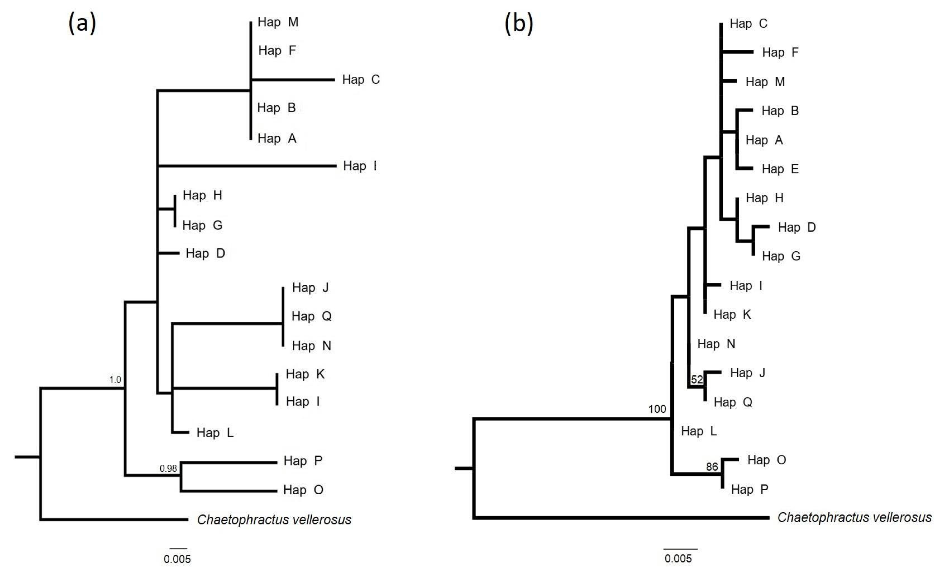
3.2. Relationships Between Haplotypes

The consensus trees of Bayesian inference and maximum likelihood showed relatively similar topologies, recovering the haplotypes O and P (Argentine province of Tucumán) in the most basal position. However, they show differences in the composition of the most derived node, the position of internal nodes and statistical support. Haplotype C in both trees is recovered in intermediate positions and low node support, indicating that the phylogenetic relationships of the total haplotypes are not fully resolved (Figure 2).
The haplotype-based genealogical relationships between peripheral and central populations represented with a haplotype network show that all Chilean sequences were recovered as haplotype C (Figure 3). Haplotype C is distributed in Chile between the provinces of Coyhaique and Magallanes (44° to 53° LS, ca. 990 km). In Argentina, this haplotype was present between the provinces of La Pampa and Tierra del Fuego (36° to 53° LS; ca. 2200 km). As in the Bayesian consensus and maximum likelihood trees (Tucumán), haplotypes O and P occupy a position at the end of the network, connecting with two mutational steps to haplotype L. Haplotype C was connected with one mutational step with haplotype F (Buenos Aires). The average Tajima’s D and Fu’s Fs values were −0.13 and 0.36, respectively, with no statistical significance (p > 0.05), suggesting that the Chilean population is in a state of demographic equilibrium and its observed genetic variation aligns with a neutral evolutionary model.

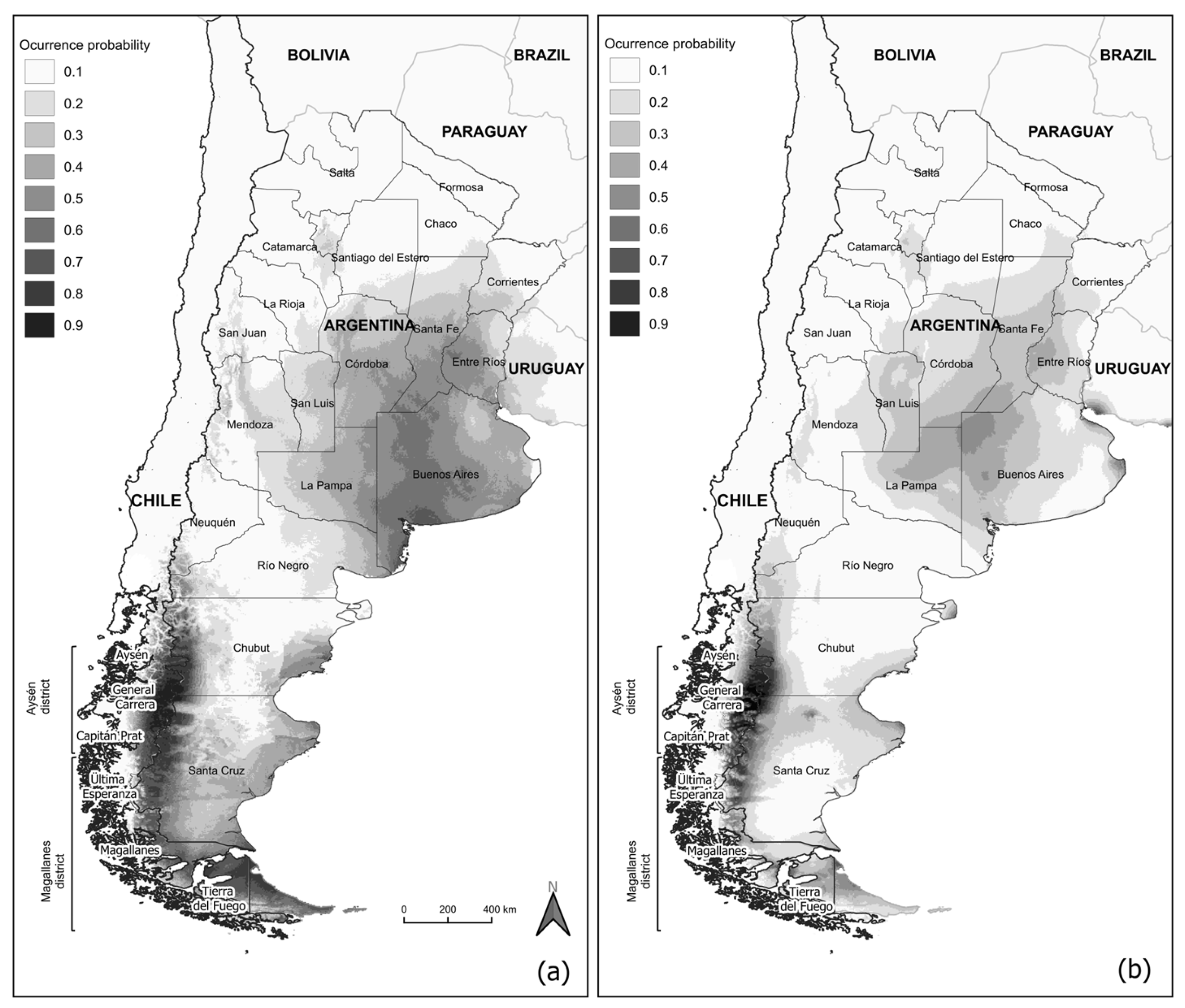
3.3. Past Geographic Distribution of C. villosus

The best-fitting Maxent model had a gain of 4.67 and a Boyce Index of 0 0.96. Also, a training AUC of 0.99, an AUC evaluation of 0.99 and a standard deviation of 0.005. The AUC values were highly similar, so the models used are appropriate for predicting the presence and absence of the species between sites. Areas with a medium/high probability of occurrence were observed in the Chilean provinces of Palena, Coyhaique, General Carrera, Capitán Prat, Última Esperanza and Magallanes, which varied between 0.6 and 1.0 (Figure 4). The Argentine sequences from the provinces of Buenos Aires, Santa Fe, Chubut, Santa Cruz and Tierra del Fuego showed similar probabilities of occurrence.
The geographic distribution predicted for the middle Holocene shows fewer areas with a probability of occurrence greater than 0.5, especially in areas that currently form part of the central distribution of the species in Argentina. The grids with probabilities greater than 0.5 were more frequent in the southern provinces of Argentina, such as Chubut and Santa Cruz, and were also present in sectors located towards the east of all the Chilean provinces of the Aysén district.

4. Discussion

4.1. Low Haplotype Diversity in Chilean Peripheral Populations

This study represents the first evaluation of the genetic diversity and genetic structure of C. villosus at the western limit of its geographical distribution. Compared with the genetic diversity reported in centrally distributed populations in Argentina [6], the peripheral population studied here exhibits low genetic polymorphism. This is demonstrated by a single haplotype being shared between the most frequent samples from Argentine Patagonian populations, including those from Chubut, Santa Cruz, and Tierra del Fuego Island [6]. This result agrees with the center–periphery model that relates lower genetic diversity in marginal areas of distribution to a reduction in gene flow and an increase in selective pressures [43,44].
Low genetic diversity in peripheral populations can arise from genetic drift, clinal genetic variation driven by habitat constraints at range edges or limited genetic exchange due to spatial isolation [43,44]. Alternatively, it may result from range retraction or the founding of populations following geographic expansion [45]. Although our analyses of Tajima’s D and Fu’s Fs showed no significant deviations from demographic equilibrium in the Chilean population, the observed low haplotype diversity in peripheral C. villosus populations, combined with their geographic proximity to Argentine Patagonian populations, suggests that a past population expansion event is the most plausible explanation for the current genetic structure.
Our genetic data along a 950 km latitudinal range represents an area not covered by previous phylogeographic studies of C. villosus, and although sample sizes could be considered low, they were sufficient to support the center–periphery hypothesis [15]. The sample size for C. villosus was limited by the low population density of the sampling area (i.e., its peripheral condition). In Chile, there is no information on the population density of C. villosus; however, studies in the Bolivian Chaco have estimated a minimum of 0.58 individuals per km2 [46], and up to 200 individuals per km2 in the Pampean region of Argentina [47]. Furthermore, behavioral characteristics shared with other armadillo species, such as their fossorial habits and crepuscular nocturnal activity, make their study and the obtaining of biological samples difficult [48].

4.2. Relationships and Geographic Distribution of Haplotypes

The phylogenetic analyses, which must be interpreted with caution given their poorly internally supported branches, and the haplotype network obtained here, were congruent. These analyses suggest that haplotypes O and P are exclusive for the Tucumán province and could be the oldest haplotypes of C. villosus. The haplotypes A, B and E seem to be derived from haplotypes found in central localities of their current distribution (the provinces of San Luis, La Pampa and Buenos Aires) [6].
All sequences identified as haplotype C were recovered in intermediate positions of the phylogenetic trees and in the haplotype network, showing closer phylogenetic relationships with the F and M haplotypes, although with low node support. The low node support can be related to the short length of the sequences (457 bp). However, the length of the sequences was sufficient to assign the peripheral sequences studied to a haplotype previously reported as C. This indicates that in well-differentiated lineages, short sequences provide good results in phylogeographic studies [49,50].
Poljak et al. [6] found haplotypes F and M in the Argentine populations from Buenos Aires and San Luis, respectively. Haplotype C was widely distributed in the current geographic range, including La Pampa, Buenos Aires, Chubut and Santa Cruz [6]; based on our study it is the only haplotype in peripheral populations in southern Chile. Considering the phylogenetic relationships, geographical proximity of the locations and environmental similarity, it is likely that the Chilean peripheral populations are the result of the dispersal of individuals westward from the Argentine provinces of Chubut and Santa Cruz.
In Chile, C. villosus is mainly distributed in the Patagonian steppe ecoregion. The peripheral individuals included in this study are found in the steppe–forest ecotone, which is characterized by an arid and cold climate [51]. Theoretically, these ecotone changes highlight the constraint for haplotype C in Chilean Patagonia; however, unpublished records show the dispersion of C. villosus to transitional valleys to the west where rainfall is greater (John Whitelaw, personal communication).

4.3. Past Geographic Distribution of C. villosus

The maximum entropy algorithm predicted that areas with medium–high environmental conditions (range 0.5 to 1.0 probability) were approximately 50% lower in warm periods of the middle Holocene than the current distribution conditions of the species. Areas with high habitability conditions were observed southward from Neuquén province during the middle Holocene (Figure 4b). The extensive area with low–medium levels of habitability between the provinces of Chubut and Santa Cruz suggests a connection between eastern populations and those of the Atlantic coast. Also, due to climatic similarities, medium–high habitability conditions were observed in areas currently occupied by the peripheral population of C. villosus distributed between Aysén and Magallanes.
The similarity of the past climates in Chilean and Argentine Patagonia is supported by palynological studies carried out in steppe–forest ecotone areas. In the Mallín Pollux location (Aysén district 45°41′30″ S 71°50′30″ W), it has been shown that 6300 years ago grasses dominated the steppe, suggesting an arid climatic condition [52]. Southward, lithological and palynological evidence obtained in Lake Casanova (47°38′36.86″ S; 72°58′30.81″ W) suggests that between 8480 and 5360 years ago the vegetation was mainly composed of a Fagaceae forest. Nonetheless, higher pollen percentages of bushes and shrubs enable us to suppose that a diversity of plants associated with open environments also developed [53]. Northward, the Argentine Mosquito Lake (42°29′37.89″ S; 71° 24′14.57″ W) and Cóndor Lake (42°20′47″ S; 71°17′07.62″ W) currently occupy the steppe–forest ecotone strip. However, between 9000 and 5230 years ago, there was a high incidence of forest fires, suggesting a predominance of dry climatic conditions dominated by sclerophyllous shrubs because of lower temperatures, with an expansion of forests of Fagaceae and other taxa towards steppe environments [54]. Thus, the vegetation changes indicate that climatic conditions affected the position of the steppe–forest ecotone, which is key to the habitat dynamics of C. villosus today. This could be a consequence of changes in the conditions of insolation, as well as the humidity derived from the advance and retreat of glaciers that affected the southern center of Patagonia, mainly the valleys and plains adjacent to the Andes [53,54].

5. Final Considerations

The habitat of the armadillo C. villosus includes slopes of the Andes, inhabiting open areas such as steppes, savannas, plains and intermontane valleys with varying degrees of anthropogenic modification. Although it is presumed that its population is stable and with a tendency towards a slight increase in its geographic ranges, its natural history is poorly documented in Chilean Patagonia. The low genetic diversity reported in the Chilean peripheral populations, combined with sighting records in Chilean Patagonia being restricted to the 20th century, are congruent with the hypothesis of a center–periphery distribution.
A consequence of this hypothesis is that peripheral populations are situated at the limit of their survival potential due to the degradation of optimal conditions across their range. As a result, these populations may act as sinks rather than sources of genetic diversity, but with a higher likelihood of extinction compared to central populations. However, their conservation value can be high because they function as a front for advance or colonization, allowing for the adjustment of a species’ distribution following climate change or environmental alterations caused by anthropogenic factors.

Supplementary Materials

The following supporting information can be downloaded at: https://www.mdpi.com/article/10.3390/d17060390/s1, Table S1. Access code to GenBank and localities related to Chilean sequences of C. villosus; Table S2. Access code to GenBank and localities related to Argentinian sequences of C. villosus [6].

Author Contributions

Conceptualization, methodology, laboratory and software analysis, writing—original draft preparation and editing, project administration and funding acquisition, A.A.; methodology, software analysis, writing—original draft preparation and editing, C.B.C.-A.; methodology, writing—original draft preparation, N.F.; methodology, C.S.; methodology, N.C. All authors have read and agreed to the published version of the manuscript.

Funding

This work was funded by project 11-I-006, “Armadillos and their presence in the Aisenina steppe: discovering the natural history of an endemic group of South American mammals”, funded by Fondo de Protección Ambiental, Ministerio del Medio Ambiente, Chile. The APC was funded by the Vicerrectoría de Investigación y Postgrado of the Universidad de Los Lagos.

Institutional Review Board Statement

Collections of biological samples of armadillos in Chile were authorized by the Servicio Agrícola y Ganadero (SAG, Chile; exempt resolutions 2048/2012 and 6956/2013).

Data Availability Statement

All relevant data are included in the paper or its Supplementary Information.

Acknowledgments

We would like to thank Conservación Patagónica, Corporación Nacional Forestal (CONAF) and Servicio Agrícola y Ganadero (SAG) for the authorizations and logistical support for the fieldwork. Our thanks also go to Eaton Lafayette for the language editing and Vicerrectoría de Investigación y Postgrado of the Universidad de Los Lagos for funding. Aldo Arriagada thanks CONICYT and the Postgraduate Department of the Universidad de Concepción for their support.

Conflicts of Interest

Cristian Saucedo was employed by the nonprofit foundation Rewilding Chile. The remaining authors declare that the research was conducted in the absence of any commercial or financial relationships that could be construed as a potential conflict of interest.

References

  1. Rabassa, J. Late Cenozoic glaciations in Patagonia and Tierra del Fuego. In The late Cenozoic of Patagonia and Tierra del Fuego; Rabassa, J., Ed.; Elsevier: Oxford, UK, 2008; pp. 151–204. [Google Scholar]
  2. Rabassa, J.; Coronato, J.; Salemme, M. Chronology of the Late Cenozoic Patagonian glaciations and their correlation with biostratigraphic units of the Pampean Region (Argentina). J. S. Am. Earth Sci. 2005, 20, 81–103. [Google Scholar] [CrossRef]
  3. Cosacov, A.; Sérsic, A.; Sosa, V.; Johnson, L.; Cocucci, A. Multiple Periglacial Refugia in the Patagonian Steppe and Post-Glacial Colonization of the Andes: The Phylogeography of Calceolaria Polyrhiza. J. Biogeogr. 2010, 37, 1463–1477. [Google Scholar] [CrossRef]
  4. Markgraf, V. Late and postglacial vegetational and paleoclimatic changes in subantarctic, temperate, and arid environments in Argentina. Palynology 1983, 7, 43–70. [Google Scholar] [CrossRef]
  5. Scillato-Yané, G. Los Dasypodidae (Mammalia, Edentata) del Plioceno y Pleistoceno de Argentina. Ph.D. Thesis, Universidad Nacional de La Plata, La Plata, Argentina, 1982; p. 159. [Google Scholar]
  6. Poljak, S.; Confalonieri, V.; Fasanella, M.; Gabrielli, M.; Lizarralde, M. Phylogeography of the armadillo Chaetophractus villosus (Dasypodidae Xenarthra): Post-glacial range expansion from Pampas to Patagonia (Argentina). Mol. Phylogenet. Evol. 2010, 55, 38–46. [Google Scholar] [CrossRef]
  7. Abba, A.; Poljak, S.; Gabrielli, M.; Teta, P.; Pardiñas, U. Armored invaders in Patagonia: Recent southward dispersion of armadillos (Cingulata, Dasypodidae). Mastozool. Neotrop. 2014, 21, 311–318. [Google Scholar]
  8. Wetzel, R. Taxonomy and distribution of armadillos, Dasypodidae. In The Ecology and Evolution of Armadillos, Sloths, and Vermilinguas; Montgomery, G., Ed.; Smithsonian Institution Press: Washington, DC, USA, 1985; pp. 23–46. [Google Scholar]
  9. Osgood, W. Mammals of Chile. Pub. Field Mus. Nat. Hist. Zool. Ser. 1943, 30, 1–268. [Google Scholar]
  10. Tamayo, M. Los armadillos de Chile. Situación de Euphractus sexcinctus (Linnaeus, 1758). Not. Mens. Del Mus. Nac. Hist. Nat. 1973, 203–204, 3–6. [Google Scholar]
  11. Arriagada, A.; Baessolo, L.; Saucedo, C.; Crespo, J.; Cerda, J.; Parra, L.; Aldridge, D.; Ojeda, J.; Hernández, A. Hábitos alimenticios de poblaciones periféricas de Zaedys pichiy y Chaetophractus villosus (Cingulata, Chlamyphoridae) en la Patagonia chilena. Iheringia Ser. Zool. 2017, 107, e2017013. [Google Scholar] [CrossRef]
  12. Poljak, S.; Escobar, J.; Deferrari, G.; Lizarralde, M. Un nuevo mamífero introducido en la Tierra Del Fuego: El Peludo Chaetophractus villosus (Mammalia, Dasypodidae) en Isla Grande. Rev. Chil. Hist. Nat. 2007, 80, 285–294. [Google Scholar] [CrossRef]
  13. Lesica, P.; Allendorf, F. When are peripheral populations valuable for conservation? when are peripheral populations valuable for conservation? Conserv. Biol. 1995, 9, 753–760. [Google Scholar] [CrossRef]
  14. Parmesan, C.; Gaines, S.; Gonzalez, L.; Kaufman, D.; Kingsolver, J.; Peterson, T.; Sagarin, R. Empirical perspectives on species borders: From traditional biogeography to global change. Oikos 2005, 108, 58–75. [Google Scholar] [CrossRef]
  15. Haak, A.; Williams, J.; Neville, H.; Dauwalter, D.; Colyer, W. Conserving peripheral trout populations: The values and risks of life on the edge. Fisheries 2010, 35, 530–549. [Google Scholar] [CrossRef]
  16. Garner, T.; Pearman, P.; Angelone, S. Genetic diversity across a vertebrate species range: A test of the central-peripheral hypothesis. Mol. Ecol. 2004, 13, 1047–1053. [Google Scholar] [CrossRef]
  17. Kirkpatrick, M.; Barton, N. Evolution of a species’ range. Am. Nat. 1997, 150, 1–23. [Google Scholar] [CrossRef]
  18. Lenormand, T. Gene flow and the limits to natural selection. Trends Ecol. Evol. 2002, 17, 183–189. [Google Scholar] [CrossRef]
  19. Yamaguchi, K.; Nakajima, M.; Taniguchi, N. Loss of genetic variation and increased population differentiation in geographically peripheral populations of japanese char Salvelinus leucomaenis. Aquaculture 2010, 308, S20–S27. [Google Scholar] [CrossRef]
  20. Hampe, A.; Petit, R. Conserving biodiversity under climate change: The rear edge matters. Ecol. Lett. 2005, 8, 461–467. [Google Scholar] [CrossRef]
  21. Volis, S.; Ormanbekova, D.; Yermekbaayev, K.; Song, M.; Shugilna, I. The conservation value of peripheral populations and a relationship between quantitative trait and molecular variation. Evol. Biol. 2015, 43, 26–36. [Google Scholar] [CrossRef]
  22. Strasburg, J.; Kearney, M.; Moritz, C.; Templeton, A. Combining phylogeography with distribution modeling: Multiple pleistocene range expansions in a parthenogenetic gecko from the Australian arid zone. PLoS ONE 2007, 2, e760. [Google Scholar] [CrossRef]
  23. John, S.; Weitzner, G.; Rozen, R.; Scriver, C. A rapid procedure for extracting genomic DNA from leukocytes. Nucleic Acids Res. 1991, 19, 408. [Google Scholar] [CrossRef]
  24. Sambrock, J.; Fritsch, E.; Maniatis, T. Molecular Cloning, a Laboratory Manual; Cold Spring Harbor Laboratory Press: New York, NY, USA, 1989. [Google Scholar]
  25. Roland, N.; Hofreiter, M. Ancient DNA extraction from bones and teeth. Nat. Protoc. 2007, 2, 1756–1762. [Google Scholar] [CrossRef]
  26. Vilá, C.; Amorin, I.; Leonard, J. Mitochondrial DNA phylogeography and population history of the grey Wolf Canis lupus. Mol. Ecol. 1999, 8, 2089–2103. [Google Scholar] [CrossRef] [PubMed]
  27. Salzburger, W.; Ewing, G.; von Haeseler, A. The performance of phylogenetic algorithms in estimating haplotype genealogies with migration. Mol. Ecol. 2011, 20, 1952–1963. [Google Scholar] [CrossRef] [PubMed]
  28. Guindon, S.; Dufayard, J.; Lefort, V.; Anisimova, M.; Hordijk, W.; Gascuel, O. New algorithms and methods to estimate maximum-likelihood phylogenies: Assessing the performance of Phyml 3.0. Syst. Biol. 2010, 59, 307–321. [Google Scholar] [CrossRef]
  29. Posada, D.; Crandall, K. MODELTEST: Testing the model of DNA substitution. Bioinformatics 1998, 14, 817–818. [Google Scholar] [CrossRef]
  30. Kumar, S.; Stecher, G.; Li, M.; Knyaz, C.; Tamura, K. MEGA X: Molecular evolutionary genetics analysis across computing platforms. Mol. Biol. Evol. 2018, 35, 1547–1549. [Google Scholar] [CrossRef]
  31. Bouckaert, R.; Heled, J.; Kühnert, D.; Vaughan, T.; Wu, C.-H.; Xie, D.; Suchard, M.A.; Rambaut, A.; Drummond, A. BEAST 2: A software platform for bayesian evolutionary analysis. PLoS Comput. Biol. 2014, 10, e1003537. [Google Scholar] [CrossRef]
  32. Fu, X. Statistical test of neutrality of mutations against population growth, hitchhiking and background selection. Genetics 1997, 147, 915–925. [Google Scholar] [CrossRef]
  33. Tajima, F. Measurement of DNA polymorphism. In Mechanisms of Molecular Evolution. Introduction to Molecular Paleopopulation Biology; Takahata, N., Clark, A., Eds.; Japan Scientific Societies Press: Tokyo, Japan; Sinauer Associates, Inc.: Sunderland, MA, USA, 1993; pp. 37–59. [Google Scholar]
  34. Rozas, J.; Ferre-Mata, A.; Sanchez-Del Barrio, J.; Guiao-Rico, S.; Librado, P.; Ramos-Onsins, S.; Sánchez-Gracia, A. DnaSP 6: DNA Sequence polymorphism analysis. Mol. Biol. Evol. 2017, 34, 3299–3302. [Google Scholar] [CrossRef]
  35. Elith, J.; Phillips, S.; Hastie, T.; Dudik, M.; Chee, Y.; Yates, C. A statistical explanation of MaxEnt for ecologists. Divers. Distrib. 2010, 17, 43–57. [Google Scholar] [CrossRef]
  36. Hijmans, R.; Cameron, S.; Parra, J.; Jones, P.; Jarvos, A. Very high resolution interpolated climate surfaces for global land areas. Int. J. Climatol. 2005, 25, 1965–1978. [Google Scholar] [CrossRef]
  37. Brown, J.L. 2014. SD Mtoolbox: A python-based GIS toolkit for landscape genetic, biogeographic and species distribution model analyses. Methods Ecol. Evol. 2014, 5, 694–700. [Google Scholar] [CrossRef]
  38. Hirzel, A.; Lay, G.; Helfer, V.; Randin, C.; Guisan, A. Evaluating the ability of habitat suitability models to predict species presences. Ecological Modelling 2006, 199, 142–152. [Google Scholar] [CrossRef]
  39. Peterson, A.; Soberón, J.; Pearson, R.; Anderson, R.; Martínez-Meyer, E.; Nakamura, M.; Araujo, M. Ecological Niches and Geographic Distributions; Princeton University Press: Princeton, NJ, USA, 2011. [Google Scholar]
  40. Pearson, R.; Raxworthy, C.; Nakamura, M.; Peterson, T. Predicting species distributions from small numbers of occurrence records: A test case using cryptic geckos in Madagascar. J. Biogeogr. 2007, 34, 102–117. [Google Scholar] [CrossRef]
  41. Boyce, M. Relating populations to habitats using resource selection functions. Ecol. Model. 2002, 157, 281–300. [Google Scholar] [CrossRef]
  42. Almalki, M.; Alrashidi, M. ¸O’Connell, M.; Shobrak, M.; Szekely, T. Modelling the distribution of wetland birds on the Red Sea coast in the Kingdom of Saudi Arabia. Appl. Ecol. Environ. Res. 2015, 13, 7–84. [Google Scholar]
  43. Eckert, C.; Samis, K.; Lougheed, S. Genetic variation across species geographical ranges: The central-marginal hypothesis and beyond. Mol. Ecol. 2008, 17, 1170–1188. [Google Scholar] [CrossRef]
  44. Dai, Q.; Fu, J. When central populations exhibit more genetic diversity than peripheral populations: A simulation study. Chin. Sci. Bull. 2011, 56, 2531–2540. [Google Scholar] [CrossRef]
  45. Quiroga, M.; Premoli, A. El rol de las poblaciones marginales en la conservación del acervo genético de la única conífera del Sur de Yungas en Argentina y Bolivia, Podocarpus parlatorei (Podocarpaceae). Ecología en Bolivia 2013, 48, 4–16. [Google Scholar]
  46. Cuéllar, E. Biology and ecology of armadillos in the Bolivian Chaco. In The Biology of the Xenarthra; Vizcaíno, S., Loughry, W., Eds.; University of Florida Press: Gainesville, FL, USA, 2008. [Google Scholar]
  47. Superina, M.; Abba, A. Family Chlamyphoridae (Chlamyphorid armadillos). In Handbook of the Mammals of the World; Wilson, D.E., Mittermeier, R.A., Eds.; Lynx Edicions: Barcelona, Spain, 2018. [Google Scholar]
  48. Mcdonough, C.; Delaney, M.; Quoc Le, P.; Blackmore, M.; Loughry, W. Burrow characteristics and habitat associations of armadillos in Brazil and the United States of America. Rev. Biol. Trop. 2000, 48, 109–120. [Google Scholar]
  49. Pilot, M.; Jedrzejewski, W.; Branicki, W.; Sidorovich, V.; Jedrzejewska, B.; Stachura, K.; Funk, S. Ecological factors influence population genetic structure of European grey wolves. Mol. Ecol. 2006, 15, 4533–4553. [Google Scholar] [CrossRef] [PubMed]
  50. Niedziałkowska, M.; Jędrzejewska, B.; Honnen, A.; Otto, T.; Sidorovich, V.; Perzanowski, K.; Skog, A.; Hartl, G.; Borowik, T.; Bunevich, A.; et al. Molecular biogeography of red deer Cervus elaphus from Eastern Europe: Insights from mitochondrial DNA sequences. Acta Theriol. 2011, 56, 1–12. [Google Scholar] [CrossRef] [PubMed]
  51. Silva, F. Caracterización y propiedades de los suelos de la Patagonia Occidental (Aysén). Boletín INIA 2014, 298, 35–52. [Google Scholar]
  52. Markraf, V.; Whitlock, C.; Haberle, S. Vegetation and fire history during the last 18,000 cal yr B.P. in Southern Patagonia: Mallín Pollux, Coyhaique, Province Aisén (45°41′30″ S, 71°50′30″ W, 640 m elevation). Palaeogeogr. Palaeoclimatol. Palaeoecol. 2007, 254, 492–507. [Google Scholar] [CrossRef]
  53. Iglesias, V.; Haberle, S.; Holz, A.; Whitlock, C. Holocene dynamics of temperate rainforests in West-Central Patagonia. Front. Ecol. Evol. 2018, 5, 177. [Google Scholar] [CrossRef]
  54. Iglesias, V.; Whitlock, C.; Bianchi, M.; Villarosa, G.; Outes, V. Holocene climate variability and environmental history at the Patagonian forest/steppe ecotone: Lago Mosquito (42°29′37.89′’S, 71°24′14.57′’W) and Laguna del Cóndor (42°20′47.22′’S, 71°17′07.62′’W). Holocene 2011, 22, 1297–1307. [Google Scholar] [CrossRef]
Figure 1. Sampling locations of peripheral individuals of C. villosus in Chile (red circles) and Argentine locations [6] (black triangles). The orange line shows the geographic range of the species.
Diversity 17 00390 g001
Figure 2. Bayesian inference consensus trees (a) and maximum likelihood (b) showing the relationships between haplotypes obtained with the mDNA control region in C. villosus.
Diversity 17 00390 g002
Figure 3. The network of haplotypes (A–Q) of C. villosus obtained from the mtDNA control region. The area of each circle is proportional to the number of individuals and is represented by curves of different sizes. The points on the blue lines represent mutation steps.
Diversity 17 00390 g003
Figure 4. Models of the potential geographic distribution of C. villosus estimated for the present (a) and the middle of the Holocene (b).
Diversity 17 00390 g004
Table 1. Sampling locations of Chaetophractus villosus specimens (n = 22) from Chile collected in this study. All individuals were recovered with haplotype C (ID: identification code for the locality of the individuals).
IDProvinceLocalityLatitudeLongitudeSample
TAP01CoyhaiqueTapera44°39′13.576″ S71°43′6.272″ Wcarcass tissue
BNU01Baño Nuevo45°15′5.764″ S71°36′54.238″ Wcarcass tissue
CAL01Coyhaique Alto45°18′16.693″ S71°23′10.9″ Wblood
LAT01Lago Atravesado45°43′27.134″ S72°13′10.175″ Wcarcass tissue
BAL01Balmaceda45°59′28.216″ S71°45′35.748″ Wcarcass tissue
BAL02Balmaceda46°1′0.293″ S71°46′7.111″ Wcarcass tissue
BAL03Balmaceda46°7′55.718″ S72°12′22.943″ Wcarcass tissue
CCA02General CarreraCerro Castillo46°6′29.005″ S72°3′8.258″ Wcarcass tissue
CCA01Cerro Castillo46°6′42.217″ S72°9′3.128″ Wblood
VIB01Valle Ibañez46°8′19.662″ S72°12′35.752″ Wcarcass tissue
VIB02Valle Ibañez46°9′40.115″ S72°21′22.81″ Wcarcass tissue
CIB01Valle Ibañez46°10′7.435″ S72°3′36.173″ Wcarcass tissue
SRI01Río Ibañez46°14′27.892″ S71°59′21.692″ Wcarcass tissue
PIB01Puerto Ibañez46°17′30.214″ S71°49′16.414″ Wcarcass tissue
CCH01Chile Chico46°34′3.774″ S71°47′40.157″ Wcarcass tissue
CJE01Sector Jeinimeni46°42′59.069″ S71°43′12.032″ Wcarcass tissue
RNJ01Sector Jeinimeni46°49′27.53″ S71°57′47.844″ Wcarcass tissue
ALE01Capitán PratLa Alegría47°8′42.72″ S72°55′17.227″ Wcarcass tissue
NEF01Río Nef47°8′47.389″ S73°2′5.244″ Wcarcass tissue
PNA01Última EsperanzaPuerto Natales51°42′54.076″ S72°27′20.372″ Wcarcass tissue
LBA01Lago Balmaceda52°1′3.256″ S72°19′59.761″ Wcarcass tissue
PUA01MagallanesPunta Arenas53°5′20.256″ S70°54′50.807″ Wcarcass tissue
Table 2. A summary of the genetic diversity indices for Chilean and Argentine populations of C. villosus based on the mtDNA control region.
Sample OriginnhSHd
Coyhaique *71000
General Carrera *101000
Capitán Prat *21000
Última Esperanza *21000
Magallanes *11000
Argentine population7617120.880.004
Argentina + Chile9817120.710.003
* = Chilean population, n = sample size, h = number haplotypes, S = polymorphic haplotypes, Hd = haplotype diversity, ∏ = nucleotide diversity.
Disclaimer/Publisher’s Note: The statements, opinions and data contained in all publications are solely those of the individual author(s) and contributor(s) and not of MDPI and/or the editor(s). MDPI and/or the editor(s) disclaim responsibility for any injury to people or property resulting from any ideas, methods, instructions or products referred to in the content.

