Abstract
Biodiversity is a foundation for maintaining ecosystem health and stability, while precise species identification is crucial to monitoring and protecting ecosystems. Subspecies of organisms, as carriers of genetic diversity, play key roles in ecosystem stability and adaptive evolution. Accurate identification of subspecies helps deepen our understanding of species distribution, ecological relationships, and change trends, providing a scientific basis for effective protection strategies. Therefore, this study proposes FineGrained-BioNet (FGBNet), a deep learning network model specifically constructed for fine-grained bio-subspecies image classification. The model combines a detail information supplement module, multi-level feature interaction, and a coordinate attention (CA) mechanism to improve the accuracy and efficiency of bio-subspecies classification. Through experimentation and optimization, the ConvNeXt is selected as the backbone network for FGBNet feature extraction, and the effectiveness of the multi-level feature interaction method is verified. Additionally, the optimal placement of the CA mechanism within the network is also explored. The experimental results show that, compared with ConvNeXt-Tiny, FGBNet achieved an increase of 6.204% in accuracy by increasing parameter quantity by only 5.702%, reaching an accuracy of 90.748%. This indicates that FGBNet significantly improves classification accuracy while maintaining computational efficiency. The proposed method facilitates more accurate subspecies classification, promoting the development of biodiversity monitoring and providing strong technical support for biodiversity conservation.
1. Introduction
Biodiversity encompasses the diversity among species, genes, and ecosystems, involving all forms of life on Earth and their ecological relationships. It serves as the foundation for life on Earth and provides humans with essential resources, such as food, fresh water, and medicines, while also maintaining crucial functions like soil fertility, water purification, and climate regulation [1]. However, since the Industrial Revolution, human activities have intensified the exploitation of natural resources, disrupting ecological balance and leading to drastic reductions in biodiversity, alongside climate change. This not only impacts the stability and integrity of nature but also poses threats to human survival and development. The preservation of biodiversity is critical for sustaining the health of ecosystems and human well-being [2,3].
Subspecies, as finer-grained classification units within species, typically represent specific evolutionary branches or adaptive changes. Their existence plays a significant role in maintaining genetic diversity and enhancing the stability of ecosystems [4,5]. Therefore, the development of more efficient and precise methods for classing subspecies of organisms is of utmost importance for the conservation of all components of biodiversity.
In recent years, more and more researchers have begun to pay attention to the application of artificial intelligence technology in biological conservation. Reference [6], introducing AI technology to integrate multi-source data and achieve preliminary detection of subspecies of organisms, solves the problems of traditional methods being time-consuming, susceptible to subjective influences, and inaccurate classification. The research system in reference [7] reviewed the methods of insect image acquisition and classification and applied techniques, such as Convolutional Neural Networks (CNNs) and Support Vector Machines (SVM), for insect subspecies recognition, avoiding the problems of subjectivity and low efficiency caused by manual recognition. In reference [8], deep learning techniques such as CNNs were utilized, combined with GPU (Graphics Processing Unit) acceleration and model optimization, to achieve high-precision classification of weeds and crops, overcoming problems such as lighting and occlusion, and achieving real-time processing and efficient recognition. Reference [9] utilizes deep learning algorithms and computer vision technologies such as SLEAP (Social Labeling Estimates Animal Poses), Argos, and drone image fusion to achieve efficient tracking and classification of animal behavior, significantly improving monitoring accuracy and real-time performance. In Reference [10], by combining traditional image processing with CNNs, the problem of time-consuming traditional acoustic fish recognition methods has been solved, achieving efficient and accurate fish species classification, and significantly improving classification accuracy and efficiency. Reference [11] utilizes CT (Computed Tomography) scanning and semantic segmentation techniques to solve the problems of time-consuming, easily contaminated, and inaccurate localization in traditional methods for detecting microplastics in organisms, achieving efficient and non-destructive detection of microplastics in fish bodies. Reference [12] utilizes deep transfer learning and multimodal techniques, such as Canny edge detection, RGB (Red, Green, Blue) color spectrum intensity analysis, and data augmentation to solve the problem of low accuracy in leaf disease detection in complex environments, significantly improving the robustness and accuracy of classification. Reference [13] explores the effectiveness of various CNNs in classifying plankton images and combines transfer learning, principal component analysis, and anomaly detection techniques to achieve efficient and accurate automatic classification of plankton images and environmental change monitoring. Reference [14] utilizes machine learning (ML) and deep learning (DL) algorithms to assess the health status of endangered delta wetlands in India, emphasizing the importance of protecting small and shallow wetlands.
From the above, it can be seen that research into the application of artificial intelligence (AI) in biodiversity conservation has gradually expanded. However, these studies primarily focus on testing the performance of various network models on certain datasets, treating AI as a tool, without proposing targeted improvement measures. Moreover, within the field of biology, research on subspecies image classification remains limited and superficial.
In terms of image classification of subspecies, the field of deep learning has accumulated a lot of research, but the conceptual framework is different. In deep learning, classification in this area typically involves the concept of fine-grained classification. Fine-grained classification is aimed at target classification problems, where the major categories are the same but the subclasses are different. For example, a challenge is how to distinguish breeds such as Husky, Samoyed, or Alaskan in dogs. By introducing the concept of fine-grained classification, researchers can develop more efficient and accurate methods for classifying subspecies of organisms, thereby better utilizing artificial intelligence technology to achieve refined ecological monitoring and scientific protection decisions.
For example, reference [15] adopts a progressive deep learning framework, combined with region focused CNNs and an attention mechanism, to study fine-grained behavior recognition of primates, solving the problem of lack of suitable datasets and complex network structures, and improving the accuracy of primate behavior recognition. Reference [16] proposes a deep convolutional feature aggregation method that combines low-level visual features and high-level semantic information to solve the problem of fine-grained variety recognition and improve the accuracy of plant species recognition. Reference [17] proposes a few-sample incremental learning method called Continuous Prototype Calibration (CPC), which effectively solves the problem of insufficient new category samples in fine-grained classification of remote sensing images and is beneficial for the recognition of new subspecies. Reference [18] utilizes deep CNNs to solve the classification problem of fly species in natural environments, improve classification accuracy, and contribute to pest control and agricultural ecological protection. Reference [19] utilizes the Vision Transformer (ViT) architecture and image processing techniques to complete fine-grained classification tasks for western flower thrips and the vegetable leafminer, improving classification accuracy and contributing to pest protection in agricultural ecological diversity. Reference [20] proposes a zero-sample learning-based method for classifying animal and plant illustrations. By constructing the ZICE (Zoological Illustration and Class Embedding) dataset and introducing fusion prototypes and hierarchical prototype losses, effective identification of rare species is achieved, promoting biodiversity research. Reference [21] manually collected bird data and enhanced it and then fed it into a CNN-based network model for category detection, achieving good experimental results. Reference [22] proposed a multi-stream hybrid architecture (MCF-Net) that utilizes a cross-level fusion strategy to achieve fine-grained crop species recognition in precision agriculture. Reference [23] proposes a fine-grained plant species classification method based on dual-view image representation and Siamese CNN, combined with a hierarchical classification strategy. This approach achieves high-precision classification and offers good scalability, making it suitable for the rapid addition of new species. Reference [24] introduces a two-stage CNN method that integrates YOLOv4(You Only Look Once Version 4) for detection and EfficientNet for identification. This method has achieved good results in the rapid classification of small herbivorous beetles, improving the efficiency and accuracy of field monitoring.
In summary, after thorough improvements, the model is capable of processing large-scale image datasets and is more suitable for application scenarios in complex field environments. However, due to the high demand for detail in fine-grained image classification, most current research focuses on enhancing classification accuracy, while neglecting speed, which is not conducive to the promotion and application of AI technology. We propose a network model that combines multi-level feature interaction, aiming to utilize relevant measures from fine-grained classification to balance the accuracy and efficiency of subspecies classification. Classification of subspecies typically involves the identification of small targets within images and the differentiation of similar targets. Semantic information alone is insufficient for distinction; substantial detail information is required for support. Therefore, we first address the needs of fine-grained classification by constructing a detail information supplement module, through which multi-level feature interaction methods are realized. Next, an attention mechanism is introduced into the feature extraction network to improve classification accuracy and model robustness. Finally, experiments are conducted to validate the effectiveness of the proposed method.
2. The Proposed Method
According to the purpose of this study and the dependence of fine-grained classification on image detail information, a method combining multi-level feature interaction is proposed to test different network models and build the FGBNet. As shown in Figure 1, in the FGBNet network, the feature fusion method is used to achieve multi-level feature interaction, and the attention mechanism is utilized to enhance the model’s ability to extract important features, thereby improving the network detection accuracy, with almost no parameter growth.
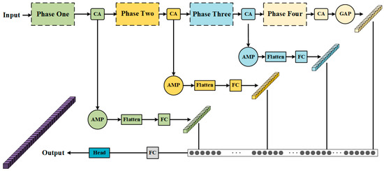
Figure 1.
Structure of FGBNet. The image is fed into the network and passes through four stages along with four multi-level feature interaction branches, ultimately producing a feature vector. This feature vector is then spatially mapped through a fully connected layer (FC). Subsequently, it undergoes activation and classification via the head, resulting in the final classification scores.
2.1. Multi-Level Feature Interaction Method
Fine-grained classification aims to identify different subcategories under the same category, and the differences between them are often very subtle. In biodiversity research, any minor morphological or textural difference may be an evolutionary clue or ecological adaptation feature, so it is necessary to ensure that the model can accurately recognize these differences. However, as CNNs increase in layers, high-level features become more semantically meaningful, while detailed information at low levels tends to gradually become lost. To improve the accuracy of subspecies classification, models not only need to utilize semantic information at high levels but also retain and use detailed information from low levels. Therefore, we propose a multi-layered feature interaction architecture that integrates features across multiple layers, ensuring sufficient semantic information, while adding more detail information, thereby enhancing the overall representation capability of the network.
The detail information supplement module is shown in Figure 2. The input features are down-sampled, flattened, and then fed to a fully connected layer for feature extraction.
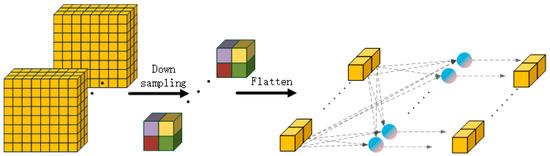
Figure 2.
Detail information supplement module. This module is utilized in each of the multi-level feature interaction branches. The module processes the input features through down-sampling, flattening, and mapping via a fully connected layer to produce a vector. Consequently, the four detail enhancement modules generate four distinct feature vectors.
If the input feature information is directly supplemented into other feature information, it will lead to an excessive number of parameters in the feature vector after the supplementation. Therefore, adaptive max pooling down-sampling is adopted to conduct preliminary screening on the input feature information. The pooled feature information is mapped through the fully connected layer to achieve further feature extraction and reduce the number of parameters in the feature vector.
The structure of multi-level feature interaction is shown in Figure 3. This structure divides input features into four levels and each level has different characteristics. Specifically, top-level features have rich detailed texture information, deep-level features have abundant semantic information, and middle-level features contain both types of information, but in different proportions. The features from shallow to deep are divided into four layers, screened and extracted by the detail information supplement module, then fused together. After fusion, the combined semantic and detail information enhances the model’s ability to detect subtle differences, thereby improving performance in subspecies identification tasks.
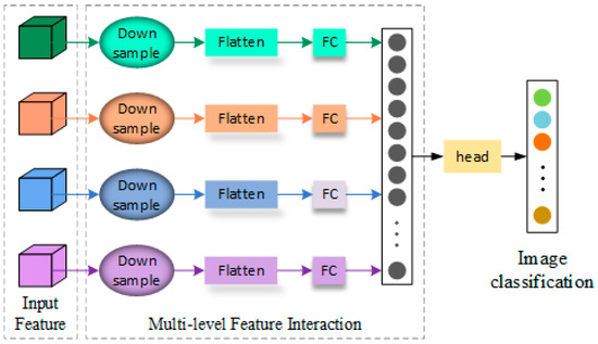
Figure 3.
Multi-level feature interaction method. The input feature on the left represents features from different levels. These features are fused through the multi-level feature interaction in the middle, which integrates information from various levels to produce a consolidated feature vector. This integrated feature vector is then fed into the head for activation and classification, ultimately yielding the final classification scores.
The detailed features obtained after passing through the detail information supplement module need to be fused. Currently, the commonly used feature fusion methods are concatenation (CONCAT), element-wise addition (ADD), and element-wise multiplication (MULTI). Suppose the feature information of the four levels to be fused are, respectively:
Then the mathematical formulae of three feature fusion are as shown in Equations (2)–(4).
In the equations, and , respectively, represent element-by-element addition and multiplication; U represents concatenation; W represents weight; and n1, n2, n3, n4, respectively, represent the length of feature vectors X1, X2, X3, X4.
As shown above, CONCAT increases feature dimensions to n-dimensions and thus enhances network expressiveness but also increases model parameters. After ADD, the dimension of features remains unchanged, and corresponding elements are added or subtracted to strengthen or weaken features, so some information is lost. MULTI creates non-linear combinations of features, which suppresses or amplifies certain features. Considering that more detailed information is needed for the subspecies classification task, we chose the CONCAT method to fuse the outputted features of four feature information supplement modules.
Due to the fact that subspecies classification mainly relies on high-level semantic information, while the enhanced detail features provided by the detail information supplement module contains more detailed texture features, it is necessary to find the proportion of different levels of information. In response to this, we changed the number of output nodes of the fully connected layer in the branches to alter the amount of features output by the branches, thereby seeking the optimal proportional relationship for multi-level feature interaction. The representation of feature vectors derived from each hierarchical level is illustrated in Equation (5):
In Equation (5), X represents input, and h, w and c denote the height, width and number of channels of the input feature, respectively. The outputsize is used to determine the output dimension after pooling. MaxPooling is a pooling function. Flatten transforms the format of the data without changing it. refers to the feature vector generated by each module after processing the input features. n1, n2, n3, n4, respectively, represent the length of the feature vectors from fully connected layers, which can also be considered as the length of the feature vectors obtained after processing the input features through various modules. i, j, k, l refer to any neuron in the fully connected layer. are the output feature vectors after pooling and flattening for model inputs, corresponding to the output feature vectors processed sequentially from shallow to deep levels. W1, W2, W3, W4 represent the weights of different modules’ fully connected layers. represent the offsets of different modules’ fully connected layers.
After sending the input feature X of each level into the detailed information supplementation branch., it first goes through a pooling layer for down-sampling and reducing the data volume. It is then flattened into one-dimensional vectors, before being sent to the fully connected layers for feature extraction. Simultaneously, the length of the output feature vectors is scaled to determine the model effects at different proportions. We will explore the best proportion relationship between n1:n2:n3:n4 in the experimental section that follows.
2.2. Feature Extraction Backbone and Attention Mechanism
In the domain of image classification, two primary approaches are commonly used: CNNs and transformers. For our tests, we selected popular models from both categories, including ResNet [25], EfficientNet [26], ConvNeXt [27], and Swin Transformer [28]. Based on these evaluations, we propose a new feature extraction network named FGBNet.
In recent years, attention mechanisms have emerged as powerful modeling tools and achieved significant success in various fields, such as natural language processing and computer vision. By dynamically weighting different parts of an input sequence, these mechanisms enable models to focus on the most relevant information for a given task. In fine-grained image classification tasks like bird subspecies identification or dog breed categorization, some subtle differences between subtypes make it difficult for traditional CNNs to capture key features. To enhance the model’s focus on local features and address challenges faced by CNNs when handling fine-grained classification tasks, we chose Coordinate Attention [29]. The CA mechanism independently processes row and column information within spatial dimensions, effectively capturing long-range dependencies in images, thereby increasing network control over overall image details.
The structure of the CA attention network is shown in Figure 4. Its core idea is to separately calculate the attention distribution along the width and height directions of the feature map. Specifically, for an input feature map , where C is the number of channels, H and W are, respectively, the height and width, and the CA attention mechanism first performs a global pooling operation on them to generate two one-dimensional vectors:
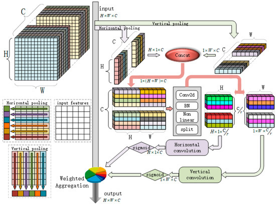
Figure 4.
Structure of CA mechanism.
Above, fh represents pooling along the width direction (i.e., horizontal direction); after pooling, the feature size is ; and width determines the pooling direction. Secondly, a 1 × 1 convolution is used to convert these two vectors in dimensionality, mapping the C dimension to an intermediate smaller dimension of to maintain computational efficiency. Finally, the Relu activation function introduces nonlinearity.
Next, the 1 × 1 convolution is again used to map the intermediate dimension r back to the original C dimension and apply a sigmoid function on the obtained result to limit the output to a [0, 1] interval, forming attention weights.
Finally, the obtained attention weights are re-applied to the original feature map to enhance or suppress the importance of specific regions. Specifically, weight aggregation is achieved by combining two weight matrices through outer product operations:
In Equation (8), denotes the outer product, which combines two vectors to form a matrix; and represents element-wise multiplication, also known as the Hadamard product.
In summary, the CA mechanism focuses on the spatial dimensions of feature maps (height and width), and independently processes row and column information, generating more precise attention weights. This enables the model to focus on key regions in an image, such as the beak or feather color of birds, improving classification accuracy and enhancing robustness against complex backgrounds and posture changes. Combined with its lightweight design, it can be introduced to improve the accuracy of the model while ensuring overall computational efficiency, which is suitable for resource-constrained environments.
3. Experimental Results and Discussion
3.1. Experimental Platform and Datasets
We tested FGBNet on a deep learning experimental platform as shown in Table 1.

Table 1.
Configuration table of deep learning experiment platform configuration table.
To validate the effectiveness of the proposed method, this paper employs several publicly available datasets for testing: Caltech-UCSD Birds-200-2011 (CUB-200-2011), Stanford Dogs, 102 Category Flower, Animals Detection Images, and iNaturalist. Parts of the datasets are shown in Figure 5.
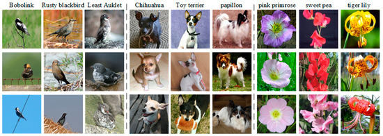
Figure 5.
Partial display of datasets.
The CUB-200-2011 dataset is an image dataset compiled by Caltech and UC San Diego about bird subspecies, and one of the widely used, fine-grained visual classification task datasets. It contains 11,788 images covering a total of 200 different bird subspecies, each associated with a Wikipedia entry and organized according to scientific classifications (including orders, families, genera, and species). Each subspecies has approximately 50 images.
The Stanford Dogs dataset contains 20,580 images of 120 different breeds and is focused on fine-grained classification tasks. This dataset is particularly suitable for subspecies classification because it covers a large number of categories that are visually similar but have subtle differences, which closely resemble morphological feature changes between subspecies of organisms.
The 102 Category Flower dataset, compiled by the Visual Geometry Group at Oxford University, consists of 8189 images spanning 102 types of flowers, organized according to botanical classifications, with approximately 80 images per class. This dataset is particularly suitable for evaluating fine-grained classification performance in distinguishing subtle morphological differences within the plant domain.
The Animals Detection Images dataset comprises a large number of annotated images covering multiple animal species, containing several thousand images. The introduction of this dataset aims to assess the model’s performance in cross-species classification tasks.
The iNaturalist dataset includes over 2 million images covering more than 100,000 species of plants and animals, making it ideal for fine-grained species classification and biodiversity studies. Each image is community-annotated, making this dataset highly suitable for testing deep learning models on species recognition and ecological research. Due to limitations in experimental resources, only a subset of this dataset was used for testing. Table 2 provides detailed information about the iNaturalist dataset.
Table 2.
Detailed information about the iNaturalist dataset.
3.2. Feature Fusion Methods
To achieve the most effective accuracy improvement, we explore the impact of different feature fusion methods on classification performance. The ConvNeXt-Tiny is used to test each type of feature fusion method and observe the change in accuracy. Table 3 indicates that the CONCAT fusion method achieves the highest accuracy.
Table 3.
Experiments with different fusion methods.
As illustrated in Figure 6, after visualizing the validation set results from the CUB-200-2011 dataset, it can be seen that both the ADD and MULTI methods exhibit a potential overfitting trend. This is because some feature information becomes weaker or disappears after being fused by ADD and MULTI, while the retained features have stronger recognizability for training sets. The generalization ability on the unseen validation set is poor, leading to an increase in loss of the validation set. However, the oscillating decreasing trend of loss on the validation set with the CONCAT method reflects that rich features pose a certain challenge to the model, which necessitates more complex dynamic adjustments during training. Therefore, it can be concluded that the CONCAT method, while achieving the highest detection accuracy, also demonstrates strong generalization ability and robustness, making it the optimal fusion approach.
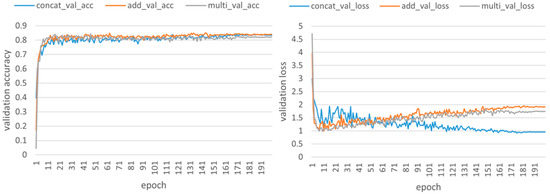
Figure 6.
Validation curves for different feature fusion methods. This figure illustrates the training curves under different feature fusion strategies. Specifically, the CONCAT method shows a continuous decrease in loss, whereas the ADD and MULTI methods exhibit an increase in loss values during training, despite improvements in accuracy. This suggests that the network remains capable of effectively recognizing images in the validation set but may be at risk of reduced discriminative power between classes. In other words, even though the model can still classify correctly, the confidence (score) of its predictions may diminish, for example, from 0.9 to 0.8. This indicates that, while classification accuracy remains unchanged, the risk of incorrect predictions increases. To summarize, although the ADD and MULTI methods also improve accuracy, they may render the model less sensitive to subtle differences.
In summary, by using the CONCAT method to combine features of different scales, not only does the model retain all original feature information but it also provides more shallow features. This allows the model to utilize information from each scale simultaneously and improve its ability to detect features of various sizes and shapes. Unlike ADD or MULTI, which may lose or compress original information, CONCAT can avoid the phenomenon where fine-grained details invade semantic information.
3.3. Proportion of Feature Information at Each Level
As shown in Figure 1, each stage of hierarchical feature information has different characteristics. Specifically, phase1 is the shallowest and retains more detailed information such as texture and edges; while phase4 is the deepest and contains more high-level semantic information. This characteristic difference makes it necessary to consider the importance of features from various stages when performing multi-stage feature interaction for feature fusion.
Since ConvNeXt-Tiny is used as a feature extraction backbone, the length of the output feature vector in Stage 4 is 768. Therefore, we set n4 = 768 when exploring proportionality relationships. So the proportionality relationship can be determined as follows:
Here, n is the length of the feature vector output by the detail information supplement module. For example, if the ratio of x is 1:1:1:1, each detail information supplement module will output a feature vector with a length of n1 = n2 = n3 = n4 = 768.
Due to the fact that the pure semantic information from stage 4 is crucial for classification, its proportion should not be too low. Therefore, experiments with a lower proportion of stage 4 were considered less. The experimental results are shown in Table 4.
Table 4.
Fusion ratio experimental results.
Experimental findings:
- (1)
- Importance of Semantic Information (n4): In experiments 2 to 5, different proportions of feature information from various stages were tested. Experiment 2, which had the richest semantic information (n4, Stage 4), performed the best. This highlights the critical role of semantic information in classification tasks.
- (2)
- Higher Accuracy with Proportional Fusion: Under the premise that semantic information is most important, we explored the impact of varying feature proportions from different stages. The results of experiments 6 to 8 show higher accuracy compared to experiment 1, which did not divide the fusion proportions. This indicates that setting proportional feature fusion enhances model performance. Among experiments 6 to 8, experiment 7, where n2 (Stage 2) had a larger proportion, showed better performance. This suggests that n2’s information is more crucial for the model. In contrast, increasing the proportions of n1 or n3 had minimal impact on accuracy improvement. Therefore, future work will focus on optimizing the proportion of n2.
- (3)
- Further Exploration of Semantic Information (n4) Proportion: Given the importance of semantic information (n4), we first investigated the optimal proportion of n4. In experiments 9 to 11, as the proportion of n4 (Stage 4) increased, model performance improved until it reached 58.33%, after which performance declined. Thus, the optimal proportion of n4 lies between 50% and 58.33%. Experiments 12, 15, and 16 further explored n4 proportions. The best n4 proportions were found to be 54.55% in experiment 10 and 53.85% in experiment 15. Therefore, the optimal n4 proportion is approximately 54%.
- (4)
- Optimal Proportion Range for n2: In experiments 14, 10, 12, and 13, with fixed ratios of n1:n3:n4 at 1:1:6, the proportion of n2 gradually increased, leading to an initial rise and subsequent decline in accuracy. Hence, the optimal proportion range for n2 is between 27.27% and 33.33%.
- (5)
- Exploration of n1 and n3 Proportions: Experiments 17 to 20 focused on exploring the proportions of n1 and n3. The highest accuracy was achieved with a ratio of 2:4:1:8.
- (6)
- This ratio includes rich pure semantic information (n4), a small amount of pure detail information (n1), a moderate amount of detail-heavy and light-semantic information (n2), and a small amount of detail-light and semantic-heavy information (n3). Such a configuration enriches and completes the features through multi-level feature interaction, thereby enhancing overall network performance.
This experiment aims to improve the accuracy of subspecies classification by optimizing the proportion of multi-level feature interaction. Considering the uniqueness of different levels of feature information, especially details in shallow features and semantic information in deep features, we designed a series of experiments to explore the best combination of each level of features. The experimental results show that properly allocating the importance of each level of features, particularly paying attention to the balance between pure semantic information (n4) and detail-heavy and light-semantic information (n2), with detail information, can significantly improve the classification performance of the model.
3.4. Feature Extraction Backbone
In this experiment, we test four popular networks (ResNet, EfficientNet, ConvNeXt and Swin Transformer) on the datasets, to evaluate the performance of different feature extraction backbones. At the same time, we apply our proposed multi-level feature interaction method (MLFI) to these networks for comparative experiments. The experimental results are shown in Table 5.
Table 5.
Experimental results with feature extraction backbones.
The experimental results show that the proposed multi-level feature interaction method can significantly improve the classification performance of different feature extraction backbone networks. It is particularly noteworthy that, after combining with multi-level feature interaction, ConvNeXt-Tiny achieves the best performance on all datasets. This indicates that, by reasonably utilizing information from different levels of features, models can enhance their ability to capture subtle differences and achieve better effects in fine-grained classification tasks. Moreover, this approach not only applies to specific network architectures but also has broad applicability to other deep learning models, demonstrating its strong generalizability and practicality, further validating the effectiveness and superiority of this method.
3.5. Comparison of Different Attention Mechanisms
To evaluate the impact of different attention mechanisms on subspecies classification tasks, we not only introduced CA in FGBNet. We also experimented with other popular attention mechanisms, including Squeeze-and-Excitation (SE) [30] attention and the Convolutional Block Attention Module (CBAM) [31]. In addition, we added these attention mechanisms at different network locations to explore their specific impacts on model performance.
First, we analyze the experimental results of the SE attention mechanism. The SE attention mechanism captures channel dependencies through global pooling operations and adjusts each channel’s importance weights by two fully connected layers. Therefore, this method can enhance key feature channels but ignores information on spatial dimensions, making it difficult to effectively handle subtle morphological differences in fine-grained classification tasks. This leads to negative growth. As shown in Table 6, the SE mechanism is insufficient for capturing local features and cannot meet complex demands in fine-grained classification tasks.
Table 6.
SE Attention mechanism.
The experimental results of the CBAM are shown in Table 7. The CBAM combines channel attention and spatial attention, first adjusts the importance of each channel through a channel attention module, then enhances or suppresses specific features through a spatial attention module. Compared with SE, CBAM can simultaneously consider both channel and spatial information but has larger computational overheads. Experimental results show that the effect of the spatial attention module is not as significant as expected. By repeatedly stacking ConvNeXt blocks to achieve high accuracy, this placement method significantly increases computation costs, which is unfavorable for deployment on low-performance platforms.
Table 7.
CBAM mechanism.
The experimental results of the CA mechanism are shown in Table 8. The CA mechanism generates attention weights containing location information by independently processing row and column information in the spatial dimension, which not only effectively captures long-range dependencies in images but also enhances local feature focus, making it more suitable for fine-grained classification tasks. Compared with SE and CBAM, CA achieves higher feature expression capability under lightweight design, focusing on key regions and subtle features to significantly improve classification accuracy.
Table 8.
CA mechanism.
The attention mechanism added within a block is usually stacked with the stacking of blocks. For example, in ConvNeXt-Tiny, the number of stackings from stage 1 to stage 4 are 3:3:9:3, so it will be stacked 27 times. Stacking multiple attention mechanisms generally helps improve model performance because more parameters mean that models can better learn complex features. However, there may be some potential issues. Adding an attention mechanism in shallow layers can enhance the extraction of low-level features as these layers mainly capture edge details and textures at this level, which makes the attention mechanism helpful in highlighting important features and improving the sensitivity of the model to subtle differences. However, its effect on enhancing high-level semantic information is limited, due to the gradual abstraction of higher-level semantics through multi-layer convolutions. Early-stage attention mechanisms might overemphasize certain local features, leading to the neglect of global structure and high-level semantics. Additionally, shallow attention mechanisms could interfere with the transmission path from lower levels to higher ones, disrupting the effective formation of high-level semantics. Therefore, compared to a model with only four CA layers, a model with 27 CA layers does not necessarily perform best, according to the experimental results shown in Table 8. The accuracy difference between the two placement methods is relatively small. Therefore, based on these considerations, it is recommended to adopt a cost-effective approach by placing the attention mechanisms after the stages.
In summary, by comparing different attention mechanisms and their placement positions, we found that the application of the CA mechanism after each stage is most effective. This is because the CA mechanism can independently process row and column information in the spatial dimension to generate more precise attention weights, thereby effectively capturing subtle features in images. In contrast, the SE mechanism only focuses on channel information, while CBAM, although it combines channel and spatial information, has a large computational overhead and insignificant spatial attention effect. Therefore, we finally chose to add the CA mechanism behind each stage, which provides an approach for improving performance in tasks such as subspecies classification in biology.
3.6. Comparative Experiments
This section summarizes the experimental data to facilitate comparison. The experiments compare the performance impact of each method on the model step-by-step, based on ConvNeXt-Tiny as a baseline. The summary results are shown in Table 9. Compared with ConvNeXt-Tiny, FGBNet increases accuracy by 6.56%.
Table 9.
Comparison experiments.
To compare the detection speed of FGBNet relative to ConvNeXt-Tiny, Table 10 lists the parameter count comparison between FGBNet and ConvNeXt-Tiny.
Table 10.
Parameter comparisons between FGBNet and ConvNeXt-Tiny.
In Table 10, “Trainable params” is the number of trainable parameters; “Non-trainable params” is the number of non-trainable parameters; “Total params” is the total number of model parameters; “Forward/backward pass size” is the temporary memory used by the model during forward/backward propagation; “Params size” is the amount of memory occupied by the model’s parameters; and “Estimated total size” is the total amount of memory required for the model to run. The average time is the average inference time after running the model 10 times.
As shown in Table 9 and Table 10, compared with ConvNeXt-Tiny, FGBNet achieves an accuracy increase of 6.56%, while only increasing the model parameters by 6.204%. The average inference time increases by 0.903 ms. Therefore, it can be concluded that the FGBNet significantly improves classification accuracy, without affecting the number of model parameters very much, maintaining computational efficiency at the same time.
To evaluate how feature attention differs between FGBNet and ConvNeXt-Tiny, this study utilized the Grad-CAM [32] method to visualize the regions that each model focuses on. The weight visualization results and feature activation localization effect are presented in Figure 7.
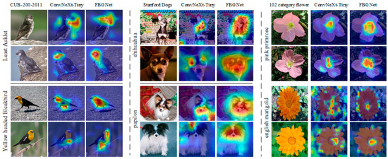
Figure 7.
Feature activation visualization effect.
As shown in the Figure 7, ConvNeXt-Tiny, before incorporating the proposed method, had limited attended regions, focused on fewer distinctive features, and paid attention to less important areas. In contrast, FGBNet, by incorporating rich detail information and the weighted attention of the CA mechanism, greatly improved these issues, leading to enhanced model accuracy.
4. Conclusions
This study proposes a fine-grained bio-Net (FGBNet) network model with multi-level feature interaction, providing an efficient and accurate subspecies classification method for the field of biodiversity conservation. FGBNet achieves significant improvements in classification accuracy and efficiency through the integration of a detail information supplement module, multi-level feature interaction methods, and the Coordinate Attention mechanism. FGBNet achieves significant improvements in classification accuracy and efficiency through the integration of a detail information supplement module, multi-level feature interaction methods, and the Coordinate Attention mechanism. Experimental results show that, on widely used datasets such as CUB-200-2011 and Stanford Dogs, FGBNet surpassed existing popular classification networks. Specifically, the precision of feature extraction backbone of ConvNeXt-Tiny is 84.544%. The precisions of ResNet50, EfficientNet-B5, Swin-Transformer-Tiny, are respectively, 83.408%, 84.31%, and 84.466%. Compared to ConvNeXt-Tiny, which is the best-performing model among the four, FGBNet increases the parameter count by only 5.702%, while achieving an accuracy improvement of 6.204%, reaching an accuracy of 90.748%. This proves that our proposed methods effectively improve the classification accuracy of the fine-grained species classification task. The subspecies classification tasks implemented by FGBNet can offer stronger support for biodiversity protection by improving the precision of ecological monitoring and facilitating scientific decision-making. Future research could further investigate FGBNet’s performance across a broader range of biological categories and optimize its real-time processing capabilities in resource-constrained environments, thereby better serving practical applications, such as species monitoring in the wild.
Author Contributions
Conceptualization, D.H.; Methodology, B.C.; Software, B.C.; Validation, D.H. and Y.S.; Formal analysis, B.C. and Y.S.; Investigation, B.C.; Resources, Y.S.; Data curation, Y.Y. and B.C.; Writing—original draft, J.W., J.X. and S.C.; Writing—review & editing, Y.Y., D.H., B.C. and Y.S.; Visualization, B.C., Y.S. and J.W.; Supervision, D.H.; Project administration, D.H.; Funding acquisition, Y.Y. and D.H. All authors have read and agreed to the published version of the manuscript.
Funding
This research was supported by the Opening Fund of the Key Laboratory of Higher Education of Sichuan Province for Enterprise Informationalization and Internet of Things (Grant No.: 2023WYJ02). Additionally, this work was also supported by the National Natural Science Foundation of China (Grant No.: 52370067).
Institutional Review Board Statement
Not applicable.
Data Availability Statement
The datasets used during the study are publicly accessible and can be accessed via the following link: CUB-200-2011: https://www.vision.caltech.edu/datasets/cub_200_2011/; Stanford Dogs: http://vision.stanford.edu/aditya86/ImageNetDogs/; Animals Detection: https://www.kaggle.com/datasets/antoreepjana/animals-detection-images-dataset; 102 Category Flower: https://www.robots.ox.ac.uk/~vgg/data/flowers/102/; iNaturalist: https://github.com/visipedia/inat_comp/tree/master/2017; All experimental data generated during the study, including the results obtained using the proposed methodology, are fully described within the ‘Experiments’ section of this manuscript. Detailed descriptions of the experiments and their outcomes are provided, ensuring transparency and reproducibility of the research findings.
Conflicts of Interest
The authors declare no conflict of interest.
References
- Lemos-Espinal, J.A.; Smith, G.R. Amphibians and Reptiles of the Pacific Lowlands Biogeographic Province of Mexico: Diversity, Similarities, and Conservation. Diversity 2024, 16, 735. [Google Scholar] [CrossRef]
- Axford, D.; Sohel, F.; Vanderklift, M.; Hodgson, A. Collectively advancing deep learning for animal detection in drone imagery: Successes, challenges, and research gaps. Ecol. Inform. 2024, 83, 102842. [Google Scholar]
- Li, L.; Liu, Y.; Wang, H.; Zhu, Y.; Li, Y.; Xu, C.; Teng, S.N. Effects of Surrounding Landscape Context on Threatened Wetland Bird Diversity at the Global Scale. Diversity 2024, 16, 738. [Google Scholar] [CrossRef]
- Lorite, J. Overharvesting Is the Leading Conservation Issue of the Endangered Flagship Species Artemisia granatensis Boiss. Diversity 2024, 16, 744. [Google Scholar] [CrossRef]
- Roswell, M.; Dushoff, J.; Winfree, R. A conceptual guide to measuring species diversity. Oikos 2021, 130, 321–338. [Google Scholar]
- Karbstein, K.; Kösters, L.; Hodač, L.; Hofmann, M.; Hörandl, E.; Tomasello, S.; Wagner, N.D.; Emerson, B.C.; Albach, D.C.; Scheu, S.; et al. Species delimitation 4.0: Integrative taxonomy meets artificial intelligence. Trends Ecol. Evol. 2024, 39, 771–784. [Google Scholar]
- Amarathunga, D.C.; Grundy, J.; Parry, H.; Dorin, A. Methods of insect image capture and classification: A systematic literature review. Smart Agric. Technol. 2021, 1, 100023. [Google Scholar]
- Adhinata, F.D.; Sumiharto, R. A comprehensive survey on weed and crop classification using machine learning and deep learning. Artif. Intell. Agric. 2024, 13, 45–63. [Google Scholar]
- Saoud, L.S.; Sultan, A.; Elmezain, M.; Heshmat, M.; Seneviratne, L.; Hussain, I. Beyond observation: Deep learning for animal behavior and ecological conservation. Ecol. Inform. 2024, 84, 102893. [Google Scholar]
- Yassir, A.; Andaloussi, S.J.; Ouchetto, O.; Mamza, K.; Serghini, M. Acoustic fish species identification using deep learning and machine learning algorithms: A systematic review. Fish. Res. 2023, 266, 106790. [Google Scholar]
- Strafella, P.; Giulietti, N.; Caputo, A.; Pandarese, G.; Castellini, P. Detection of microplastics in fish using computed tomography and deep learning. Heliyon 2024, 10, e39875. [Google Scholar]
- Ametefe, D.S.; Sarnin, S.S.; Ali, D.M.; Caliskan, A.; Caliskan, I.T.; Aliu, A.A.; John, D. Enhancing leaf disease detection accuracy through synergistic integration of deep transfer learning and multimodal techniques. Inf. Process. Agric. 2024; in press. [Google Scholar]
- Ciranni, M.; Murino, V.; Odone, F.; Pastore, V.P. Computer vision and deep learning meet plankton: Milestones and future directions. Image Vis. Comput. 2024, 143, 104934. [Google Scholar]
- Paul, S.; Pal, S. Mapping wetland habitat health in moribund deltaic India using machine learning and deep learning algorithms. Ecohydrol. Hydrobiol. 2024, 24, 667–680. [Google Scholar]
- Feng, J.; Luo, H.; Fang, D. A progressive deep learning framework for fine-grained primate behavior recognition. Appl. Anim. Behav. Sci. 2023, 269, 106099. [Google Scholar]
- Wu, H.; Fang, L.; Yu, Q.; Yang, C. Deep convolutional feature aggregation for fine-grained cultivar recognition. Knowl.-Based Syst. 2023, 275, 110688. [Google Scholar]
- Zhu, Z.; Wang, P.; Diao, W.; Yang, J.; Wang, H.; Sun, X. Few-shot incremental learning with continual prototype calibration for remote sensing image fine-grained classification. ISPRS J. Photogramm. Remote Sens. 2023, 196, 210–227. [Google Scholar]
- Chen, Y.; Zhang, X.; Chen, Z.; Song, M.; Wang, J. Fine-grained classification of fly species in the natural environment based on deep convolutional neural network. Comput. Biol. Med. 2021, 135, 104655. [Google Scholar]
- Amarathunga, D.C.; Ratnayake, M.N.; Grundy, J.; Dorin, A. Fine-grained image classification of microscopic insect pest species: Western flower thrips and plague thrips. Comput. Electron. Agric. 2022, 203, 107462. [Google Scholar]
- Stork, L.; Weber, A.; van den Herik, J.; Plaat, A.; Verbeek, F.; Wolstencroft, K. Large-scale zero-shot learning in the wild: Classifying zoological illustrations. Ecol. Inform. 2021, 62, 101222. [Google Scholar]
- Alfatemi, A.; Jamal SA, L.; Paykari, N.; Rahouti, M.; Chehri, A. Multi-Label Classification with Deep Learning and Manual Data Collection for Identifying Similar Bird Species. Procedia Comput. Sci. 2024, 246, 558–565. [Google Scholar]
- Kong, J.; Wang, H.; Wang, X.; Jin, X.; Fang, X.; Lin, S. Multi-stream hybrid architecture based on cross-level fusion strategy for fine-grained crop species recognition in precision agriculture. Comput. Electron. Agric. 2021, 185, 106134. [Google Scholar]
- Araújo, V.M.; Britto Jr, A.S.; Oliveira, L.S.; Koerich, A.L. Two-view fine-grained classification of plant species. Neurocomputing 2022, 467, 427–441. [Google Scholar]
- Takimoto, H.; Sato, Y.; Nagano, A.J.; Shimizu, K.K.; Kanagawa, A. Using a two-stage convolutional neural network to rapidly identify tiny herbivorous beetles in the field. Ecol. Inform. 2021, 66, 101466. [Google Scholar]
- He, K.; Zhang, X.; Ren, S.; Sun, J. Deep residual learning for image recognition. In Proceedings of the IEEE Conference on Computer Vision and Pattern Recognition, Las Vegas, NV, USA, 27–30 June 2016; pp. 770–778. [Google Scholar]
- Tan, M.; Le, Q. Efficientnet: Rethinking model scaling for convolutional neural networks. In Proceedings of the International Conference on Machine Learning, PMLR, Long Beach, CA, USA, 9–15 June 2019; pp. 6105–6114. [Google Scholar]
- Liu, Z.; Mao, H.; Wu, C.Y.; Feichtenhofer, C.; Darrell, T.; Xie, S. A convnet for the 2020s. In Proceedings of the IEEE/CVF Conference on Computer Vision and Pattern Recognition, New Orleans, LA, USA, 18–24 June 2022; pp. 11976–11986. [Google Scholar]
- Liu, Z.; Lin, Y.; Cao, Y.; Hu, H.; Wei, Y.; Zhang, Z.; Lin, S.; Guo, B. Swin transformer: Hierarchical vision transformer using shifted windows. In Proceedings of the IEEE/CVF International Conference on Computer Vision, Montreal, QC, Canada, 10–17 October 2021; pp. 10012–10022. [Google Scholar]
- Hou, Q.; Zhou, D.; Feng, J. Coordinate attention for efficient mobile network design. In Proceedings of the IEEE/CVF Conference on Computer Vision and Pattern Recognition, Nashville, TN, USA, 20–25 June 2021; pp. 13713–13722. [Google Scholar]
- Hu, J.; Shen, L.; Sun, G. Squeeze-and-excitation networks. In Proceedings of the IEEE Conference on Computer Vision and Pattern Recognition, Salt Lake City, UT, USA, 18–23 June 2018; pp. 7132–7141. [Google Scholar]
- Woo, S.; Park, J.; Lee, J.Y.; Kweon, I.S. Cbam: Convolutional block attention module. In Proceedings of the European conference on computer vision (ECCV), Munich, Germany, 8–14 September 2018; pp. 3–19. [Google Scholar]
- Selvaraju, R.R.; Cogswell, M.; Das, A.; Vedantam, R.; Parikh, D.; Batra, D. Grad-cam: Visual explanations from deep networks via gradient-based localization. In Proceedings of the IEEE international Conference on Computer Vision, Venice, Italy, 22–29 October 2017; pp. 618–626. [Google Scholar]
Disclaimer/Publisher’s Note: The statements, opinions and data contained in all publications are solely those of the individual author(s) and contributor(s) and not of MDPI and/or the editor(s). MDPI and/or the editor(s) disclaim responsibility for any injury to people or property resulting from any ideas, methods, instructions or products referred to in the content. |
© 2025 by the authors. Licensee MDPI, Basel, Switzerland. This article is an open access article distributed under the terms and conditions of the Creative Commons Attribution (CC BY) license (https://creativecommons.org/licenses/by/4.0/).