The Optimal Counting Number for Silicoflagellate Assemblages in the Western Arctic Ocean

Abstract

Siliceous plankton are vital for understanding modern and past marine environments. However, few studies have been carried out on silicoflagellates, a group of siliceous phytoplankton. The determination of reliable environmental reconstructions using silicoflagellates is hindered by the lack of consensus on the optimal counting number. In this study, sinking particles and surface sediments collected from the Chukchi Sea, western Arctic Ocean, were used to investigate the composition of silicoflagellates and to determine the optimal counting number of silicoflagellate assemblages. The silicoflagellate assemblage in the western Arctic is dominated by Octactis speculum, followed by Staphanocha medianoctisol in secondary abundance, while Octactis octonaria and Stephanocha quinquangella are present in very low frequencies. Employing an analysis of relative abundances and their corresponding coefficient of variations (CVs) for different silicoflagellate species across a counting gradient, we established an optimal counting number of 100–200 silicoflagellate skeletons for samples with high abundance. In contrast, the entire sample slide should be counted due to the low absolute abundance of silicoflagellates in surface sediments.

1. Introduction

In recent decades, the Arctic Ocean has been warming at a rate of two to four times faster than the global average [1,2,3,4]. The Arctic summer sea ice has been melting rapidly, with its largest extent declining by 13.3% per decade [5]. These environmental changes have consequently caused dramatic shifts in local marine ecosystems [6,7,8]. Owing to the expansion of open water areas, annual net primary productivity in the Arctic Ocean has increased by 30% [9]. Moreover, a decreasing trend in phytoplankton size has been observed during summer in the Chukchi Sea [10].

Silicoflagellates are defined as planktonic unicellular algae with chloroplasts and a single flagellum [11]; they are characterized by a polygonal silica skeleton with diameters ranging from 20 to 100 μm [11]. The silica skeletons can be buried in marine sediments for long periods, thereby preserving environmental information [11,12]. Among other siliceous plankton, diatoms and radiolarians are frequently used in environmental research in the Arctic Ocean [13,14,15,16,17,18,19,20]. However, silicoflagellates have been reported only sporadically [21,22,23], limiting their use as indicators of changes in the marine environment. In the Arctic Ocean, silicoflagellate assemblages are dominated by a few species, namely, Octactis speculum (Ehrenberg) F.H. Chang, J.M. Grieve & J.E. Sutherland, Stephanocha medianoctisol (K. Takahashi, Onodera & Katsuki) K. McCartney & R.W. Jordan, O. octonaria (Ehrenberg) Hovasse, and S. quinquangella (Bukry & J.H. Foster) K. McCartney & R.W. Jordan, along with a small number of variants (Figure 1) [21,22,23]. Previous researches have revealed a seasonal pattern in silicoflagellate assemblages within sinking particles, characterized by the dominance of O. speculum in summer and a notable increase of S. medianoctisol and O. octonaria during winter [22,23]. Recent studies on Arctic silicoflagellates have focused mostly on seawater and sea ice samples [21,22,23,24], leaving their distributions in surface sediments generally unknown [21,22,23].

In contrast to common siliceous plankton, such as diatoms and radiolarians, the optimal counting number for silicoflagellate assemblages remains unexplored. For diatoms, a count of 300–400 valves per sample is generally considered statistically significant [18,19,20,25,26]. Previous studies utilizing silicoflagellate assemblages in sinking particles and sediments from the Arctic and North Pacific Oceans as environmental indicators have employed minimum counting numbers ranging from 50 to 400 skeletons [12,23,27,28,29,30,31]. However, the rationale behind these thresholds remains unclear. This lack of a well-defined and practical optimal counting number hinders the reliable application of silicoflagellates as robust proxies for environmental changes in the Arctic Ocean and other regions.

In this study, we establish several counting gradients for silicoflagellate assemblages using samples from sinking particles and surface sediments to determine the optimal counting number for silicoflagellate assemblages in both seawater and sediments in the Arctic Ocean.

2. Materials and Methods

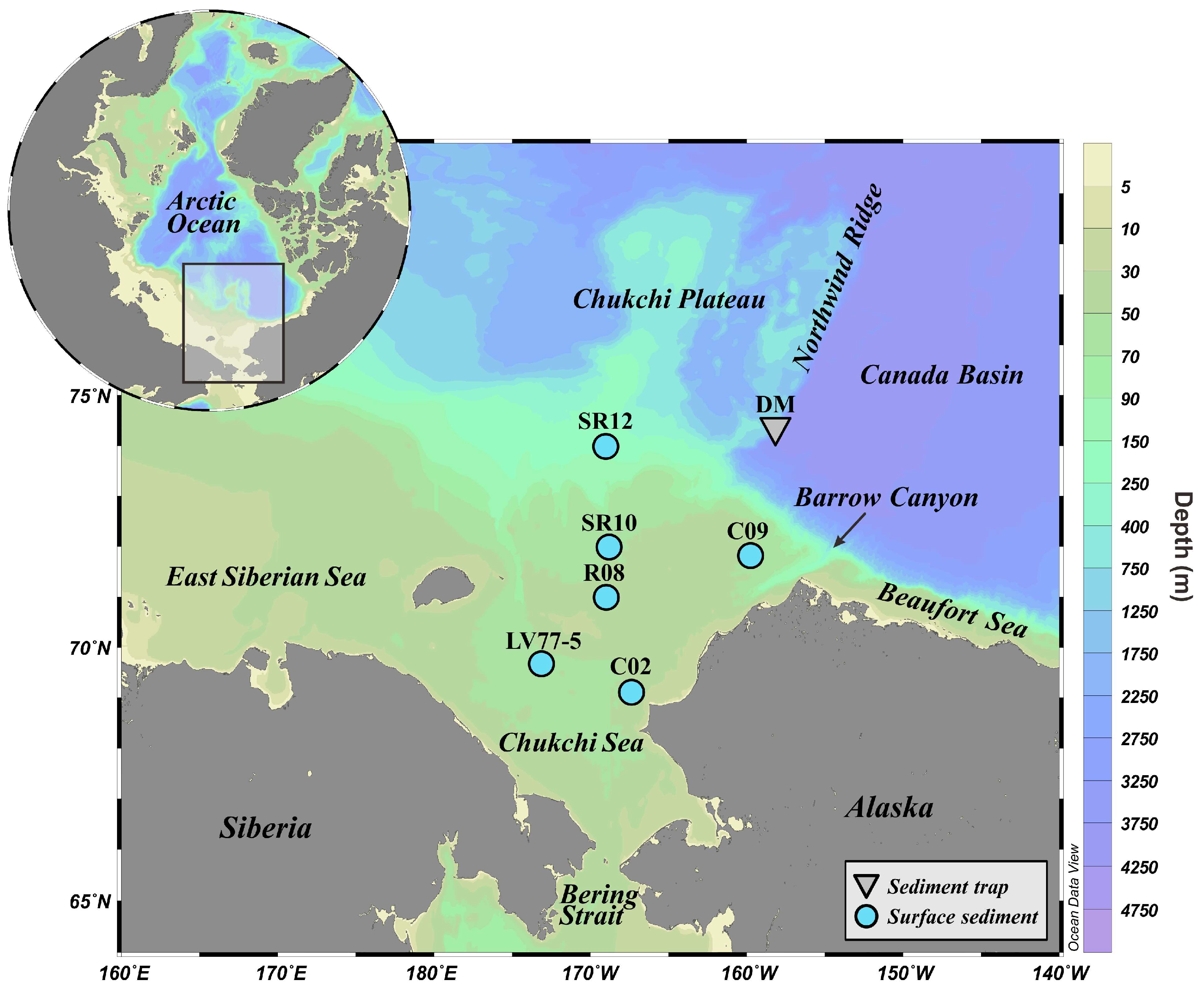
2.1. Oceanographic Setting

The Chukchi Sea is one of the marginal seas of the Arctic Ocean [32]. It is connected to the Bering Sea through the Bering Strait in the south (Figure 2) [33]. The Chukchi Sea is mostly shallow, with an average depth of ~50 m [33].

The Chukchi Sea is strongly influenced by the nutrient-rich inflow of Pacific water [34], making it one of the most productive marginal seas of the Arctic Ocean [35]. The Siberian Coastal Current, which flows across the eastern Siberian shelf, brings low-salinity water to the Chukchi Sea [36]. Additionally, the anticyclonic Beaufort Gyre also carries less saline water to the Chukchi Sea [37]. The Chukchi Sea is characterized by seasonal sea ice [38], which begins to form in October. The region is entirely ice-covered from December through April of the following year. Melting starts in May, with the sea ice reaching its minimum extent by September, leaving the entire Chukchi Sea ice free [39,40].

2.2. Sinking Particles and Surface Sediments

Sinking particles were collected by a year-round sediment trap (McLane PARFLUX Mark 78H-21) deployed at Station DM (74°24.0′ N, 158°14.0′ W, trap depth 870 m, water depth 1650 m) on the Northwind Ridge during the 3rd Chinese National Arctic Research Expedition (CHINARE; Figure 2). The sediment trap was equipped with 21 sampling cups. In general, these cups were set to rotate automatically every two weeks from July to November or one month from December to June to collect sinking particles for corresponding time windows. Six samples representing different marine environments were selected for further study (

Table 1. Selected sinking particle samples collected by the sediment trap.

No. of Cup	Periods of Collection	Environment
1#	7 August 2008–15 August 2008	Ice-free
3#	1 September 2008–15 September 2008	Ice-free
21#	16 September 2009–30 September 2009	Ice-free
7#	1 November 2008–15 November 2008	Frozen
17#	16 July 2009–31 July 2009	Ice melting
18#	1 August 2009–15 August 2009	Ice melting

).

Six surface sediment samples from the Chukchi Shelf, which were collected using a box corer during the 4th and 5th CHINARE and the 1st Sino-Russian Joint Arctic Expedition (LV77), were also analyzed (Figure 2).

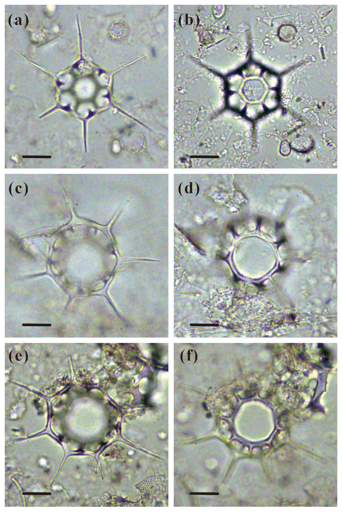
2.3. Slide Preparation and Identification of Silicoflagellates

For sinking particles, microscope slides for the investigation of silicoflagellates were made as described in Ren et al. (2021) [23].

For surface sediments, the preparation process was as follows: (a) Pretreatment: This process was carried out mainly according to Kato et al. (2023) [41]. Approximately 1 g of dry sample was placed into a 50 mL centrifuge tube. Then, 30% H₂O₂ was added, and the mixture was heated at 70 °C in a water bath for 6 h to remove the organic matter. After washing with distilled water, 5% HCl was added, and the mixture was left at room temperature for 12 h to remove the calcareous material. (b) Sieving: Each sample was filtered with 1000 mesh (~13 μm in pore size) and rinsed with distilled water. (c) Heavy liquid separation: Zinc bromide (ZnBr₂) was used as the heavy liquid medium (target density: 2.3–2.4 g/cm³). Appropriate drops of heavy liquid were pipetted into each sample. After mixing and centrifuging, the supernatant was collected. This step was repeated several times to achieve separation of siliceous plankton (including silicoflagellates) and clay minerals. d) Slide preparation: A certain aliquot of the sample residue was dropped on a cover glass, which was mounted with Norland Optical Adhesive 61 (NOA 61, $n_D~1.56$).

All the slides were observed under a Motic BA410 microscope (Motic Electric, Xiamen, China) at ×400 magnification. Only silicoflagellates with intact skeletons were counted.

2.4. Counting Quadrat and Gradient Setting

A counting quadrat was defined as 50 silicoflagellate skeletons along transects. Typically, 8 counting quadrats, totaling 400 skeletons, were counted for each sample, except for samples with fewer skeletons. Accordingly, counting gradients for silicoflagellate skeletons in sinking particles and surface sediments were established at multiples of the counting quadrats (starting at 1 quadrat, i.e., 50 skeletons). If the number of silicoflagellate skeletons on one slide fell below the minimum counting gradient, the quantity was insufficient for counting gradient steps. In such cases, entire slide counting was required.

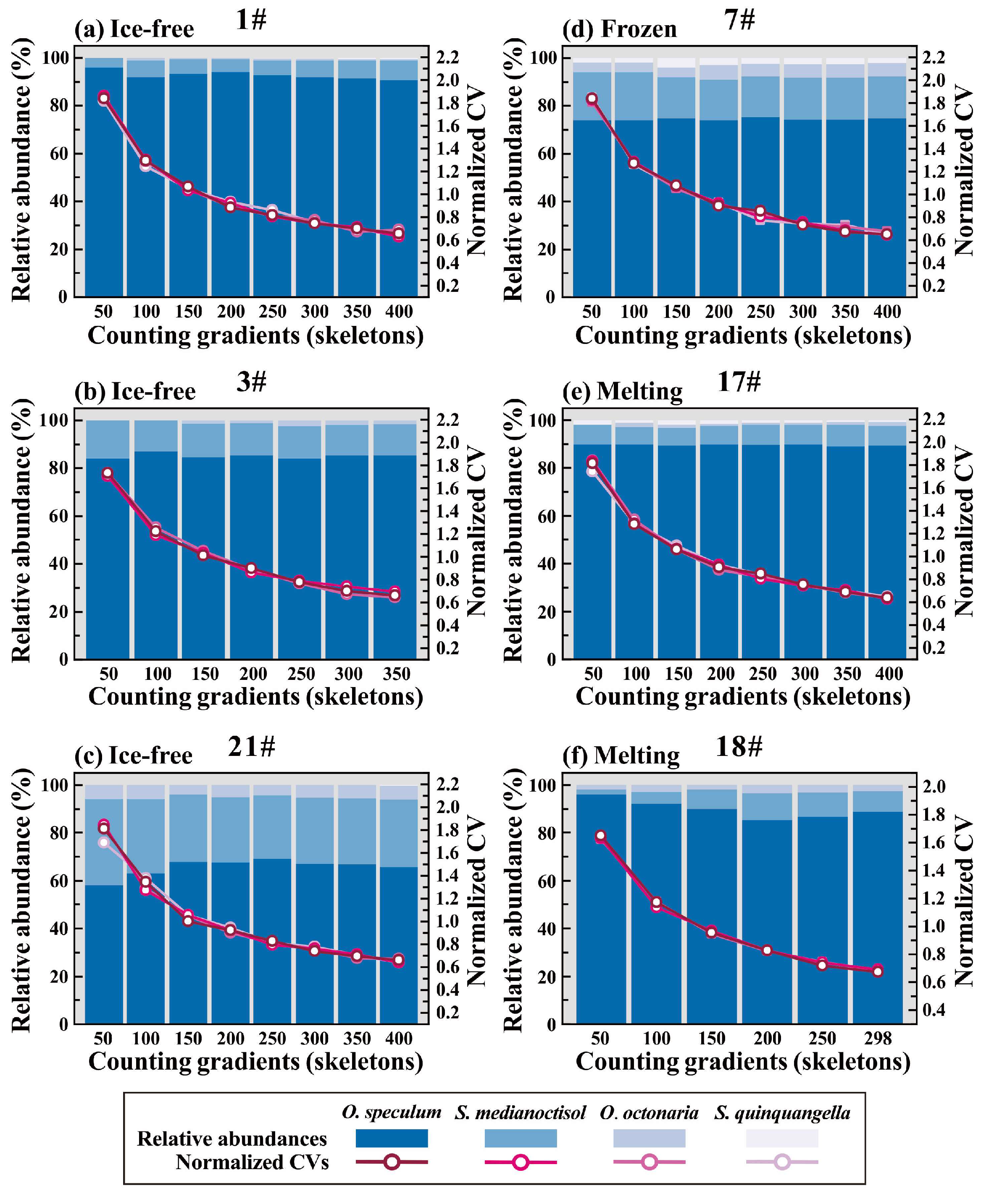
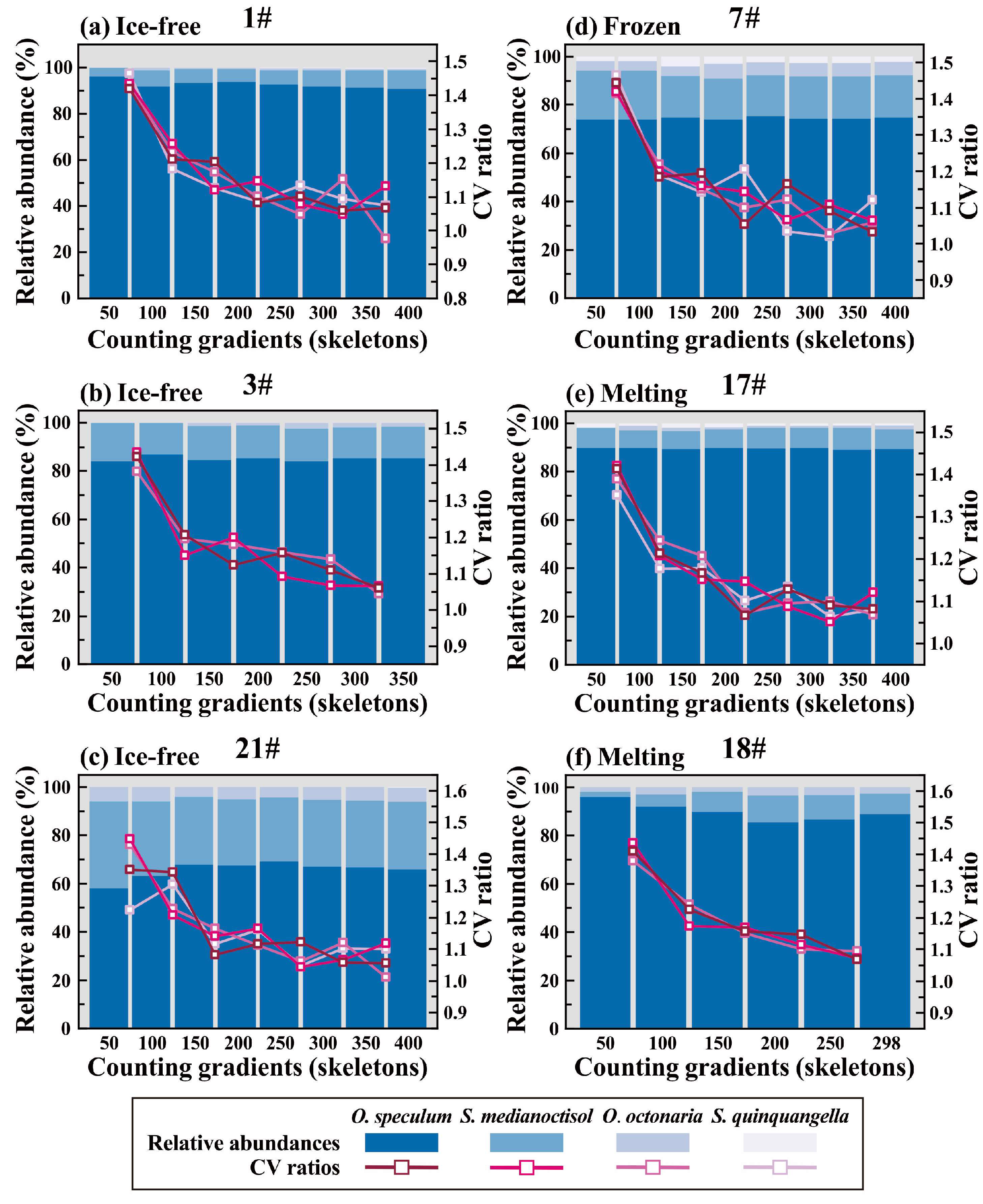
2.5. Optimal Counting Number Determination

The relative abundances, their coefficient of variations (CVs), and corresponding change ratios of different silicoflagellate species were used to determine the optimal counting numbers for silicoflagellate assemblages.

CVs are inspired by concepts of ecosystem diversity and stability in ecological studies (e.g., Tilman, 1996; Tilman et al., 1998) [42,43]. In principle, CV represents the variation against the mean abundance of a particular species along the counting gradient. It serves as an index for the variability of species relative abundances across different counting gradients.

Practically, i counting quadrats (1 ≤ i ≤ 8) were randomly selected from a total of 8 quadrats, and the mean relative abundance of specie x (denoted as P) was calculated. This process was iterated for 1000 times. The standard deviation and mean of these 1000 P values were calculated as σ_x|i and μ_x|i, respectively. The CV_x|i was then calculated using the following formula:

$$C{V}_{x|i}={\displaystyle \frac{{\sigma }_{x|i}}{{\mu }_{x|i}}}$$

(1)

where x represents the target species, and i is the counting gradient number, σ and μ are the standard deviation and the mean of the relative abundance of species x along the counting gradient i, respectively. To minimize the influence of inherent variations in species’ relative abundances on CVs, they were normalized as ratios between CV_x|i and the average CV calculated from all eight quadrats. Additionally, the CV change ratios were calculated as ratios between CV_x|i+1 and CV_x|i to indicate the relative change in CVs across different counting gradients. Stabilized states of normalized CVs and CV change ratios at counting gradient i suggest that i counting quadrats may statistically represent the entire assemblage, and therefore, indicate the optimal counting number.

The calculations were performed using Resampling Stats 4.0, an add-in for Excel [44].

3. Results and Discussion

3.1. Silicoflagellates in Insinking Particles

Four silicoflagellate species were identified in all six samples of sinking particles. The silicoflagellate assemblages were dominated by O. speculum (Figure 3; Table S1), despite the seasonal variations in different species reported in previous studies [22,23]. In addition, except for samples 3# and 18#, which had fewer than 400 silicoflagellate skeletons on all the slides (3#: 358; 18#: 298; all in skeletons), all the remaining four samples had more than 400 skeletons (1#: 483; 7#: 665; 17#: 656; 21#: 1319; all in skeletons). In addition, O. speculum and S. medianoctisol accounted for more than 90% of the silicoflagellate assemblages. Therefore, the changes in the relative abundances of O. speculum and S. medianoctisol can be used as references for the optimal counting number.

The relative abundances of O. speculum in each counting gradient of the six sinking particle samples ranged from 58% to 96%, whereas those of S. medianoctisol ranged from 2% to 36% (Figure 3; Table S1). In sample 18#, the relative abundance of O. speculum decreased with increasing counting gradient, and the relative abundance of S. medianoctisol increased, but both level off at a counting gradient of 200. In contrast, the relative abundance of O. speculum increased with increasing counting gradient, and the relative abundance of S. medianoctisol decreased in sample 21# and then reached a plateau at a counting gradient of 150. The relative abundances of the silicoflagellates in each counting gradient of the remaining four samples were relatively stable. Apparently, the overall changes in the relative abundances of O. speculum and S. medianoctisol along with increasing counting gradients were not statistically significant.

The change ratio of relative abundances (CRA) for a specific species is defined as the ratio of the relative abundances of that species between two adjacent counting gradients within a single sample. For the 21# sample, the CRA of O. speculum became stable after a counting gradient of 150. In contrast, the CRAs of the remaining five O. speculum samples stabilized at a counting gradient of 50 (Figure S1). It is apparent that the trends of the CRAs and relative abundances of O. speculum were coupled in most samples. Exceptions were encountered in the 1# and 18# samples. The relative abundances of O. speculum in the 1# and 18# samples reached their peak values at a counting gradient of 50 and decreased with increasing counting gradients until they reached a steady state at counting gradients of 150–200 (Figure S1). The secondary dominant species, S. medianoctisol, showed greater fluctuations in relative abundance and CRA (Figure S1). Most samples had a high (1# and 18#) or low (3#, 17#, and 21#) CRA at a counting gradient of 50 and then started to decline or rise to a stable state along with an increasing counting gradient (Figure S1). The low CRA of the 7# sample, however, occurred at a counting gradient of 100 and subsequently increased to a stable state (Figure S1).

In addition, the normalized CVs of four silicoflagellate species exhibited consistent patterns across all six samples, despite minor variations (Figure 3). They consistently decreased from the first counting gradient but gradually stabilized as the gradient increased (Figure 3). Notably, the most pronounced drops in normalized CVs occurred between the first two counting gradients (100 skeletons) in most samples, while in sample 21#, the steepest decline extended to the first three gradients (150 skeletons; Figure 3). The CV change ratios of all species followed a similar trend to the normalized CVs (Figure 4). High values were observed in the initial counting gradients, followed by a leveling off with values ranging between 1.1 and 1.0, indicating negligible changes of CVs along the subsequent gradients. This suggests that the composition of silicoflagellate assemblage remained stable and likely represents the whole assemblage in the sample. Therefore, the first gradient at which the CV change ratios stabilized was defined as the optimal counting number, ranging from 100 to 200 skeletons across the six samples (Figure 4).

In summary, the relative abundances, their CVs, and corresponding change ratios of all silicoflagellate species were generally stable at counting gradients ranging from 100 to 200. Consequently, for Arctic Ocean samples with a high abundance of silicoflagellates, counting between 100 and 200 skeletons optimally may represent the entire silicoflagellate assemblage. This result aligns with previous studies that has employed silicoflagellates as environment indicators in both the Arctic and North Pacific Oceans [12,23,29,31], and may contribute to the paleoenvironmental reconstructions based on silicoflagellate assemblages. However, the optimal counting number likely varies depending on the diversity of the silicoflagellate assemblage. In regions with greater silicoflagellate species richness, a higher optimal counting number may be required to adequately represent the entire assemblage and thus accurately reflect environmental conditions.

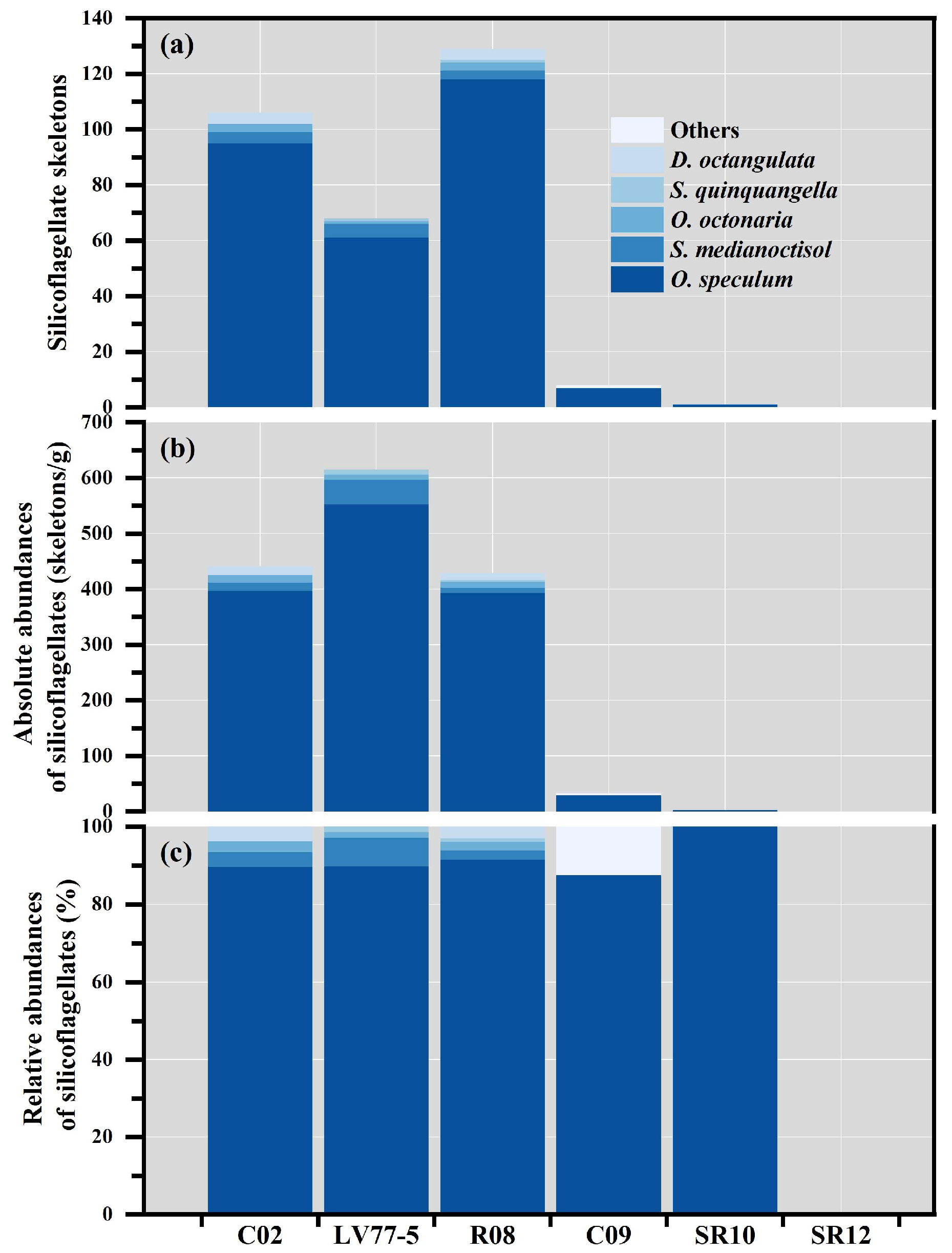
3.2. Silicoflagellates in the Surface Sediments

Silicoflagellates were abundant in three surface sediment samples (C02: 106; LV77-5: 68; R08: 129; all in skeletons), and three major species were identified (Figure 5a). In the remaining three samples, a very small number of silicoflagellate skeletons were observed or were even absent (C09: 8; SR10:1; SR12: 0; all in skeletons). Only O. speculum was observed in these samples (Figure 5a and Figure 6, and

Table 2. Skeletons, absolute and relative abundances of silicoflagellates in surface sediment samples.

Stations		Silicoflagellate Species
		O. speculum	S. medianoctisol	O. octonaria	S. quinquangella	D. octangulata	Others
C02	Total skeletons	95	4	3	n.o	4	n.o
	Absolute abundance (skeletons/g)	396	16	13	n.o	16	n.o
	Relative abundance (%)	89.60	3.80	2.80	n.o	3.80	n.o
LV77-5	Total skeletons	61	5	1	1	n.o	n.o
	Absolute abundance (skeletons/g)	553	44	9	9	n.o	n.o
	Relative abundance (%)	89.71	7.35	1.47	1.47	n.o	n.o
R08	Total skeletons	118	3	3	1	4	n.o
	Absolute abundance (skeletons/g)	393	10	10	3	13	n.o
	Relative abundance (%)	91.50	2.30	2.30	0.80	3.10	n.o
C09	Total skeletons	7	n.o	n.o	n.o	n.o	1
	Absolute abundance (skeletons/g)	29	n.o	n.o	n.o	n.o	4
	Relative abundance (%)	87.50	n.o	n.o	n.o	n.o	12.50
SR10	Total skeletons	1	n.o	n.o	n.o	n.o	n.o
	Absolute abundance (skeletons/g)	4	n.o	n.o	n.o	n.o	n.o
	Relative abundance (%)	100	n.o	n.o	n.o	n.o	n.o
SR12	Total skeletons	n.o	n.o	n.o	n.o	n.o	n.o
	Absolute abundance (skeletons/g)	n.o	n.o	n.o	n.o	n.o	n.o
	Relative abundance (%)	n.o	n.o	n.o	n.o	n.o	n.o

n.o: not observed.

). Consequently, the absolute abundances of silicoflagellates were high in the first three samples (C02: 441; LV77-5: 615; R08: 429; all in skeletons/g), whereas those of the remaining three samples were extremely low or absent (C09: 33; SR10: 4; SR12: absent; all in skeletons/g) (Figure 5b and Figure 6, and Table 2). Low levels of biogenic silica were measured in C09 and SR12, which is likely related to the low absolute abundance of silicoflagellates in these samples [45].

The silicoflagellate assemblages in the six surface sediment samples were dominated by O. speculum, with relative abundances greater than 89%, whereas those of S. medianoctisol, O. octonaria and Dictyocha octangulata (Wailes) McCartney were lower than 10% (Figure 5c and Figure 6, and Table 2). The silicoflagellate composition of surface sediments was slightly different from that of the aforementioned sinking particles (Figure 3). The difference in the silicoflagellate assemblages in the sinking particles and surface sediments might be a consequence of differential dissolution of the silicoflagellate skeletons. Similar to diatom valves, silicoflagellate skeletons are susceptible to dissolution within water columns and sediments under specific environmental conditions. The dissolution process can also be accelerated by bacterial activities [11,46,47]. In addition, S. medianoctisol and O. octonaria, which have subtle skeleton structures, may be more vulnerable to dissolution. In comparison, O. speculum, which has a simple skeleton structure, is robust and has good preservation in sediments. Furthermore, different silicoflagellate species prefer varying seawater environments. For example, O. speculum is abundant in temperate and cold regions, whereas S. medianoctisol and O. octonaria favor much icier environments [12,21,22,23,29,48]. Thus, the silicoflagellate assemblages of the sinking particle samples, which were collected over the Northwind Ridge, are obviously different from those of the surface sediment samples from the Chukchi Shelf (Figure 2), indicating varying environmental settings.

The number of silicoflagellate skeletons in samples C02 and R08 exceeded 100, whereas in the remaining four samples, the number of skeletons was generally less than 70, making it impossible to perform gradient counting experiments (Table 2; Figure 5). Therefore, for samples with low silicoflagellate abundance in the western Arctic Ocean, entire slide observations and counting are necessary.

4. Conclusions

We analyzed silicoflagellate assemblages in samples of sinking particles and surface sediments from the Chukchi Sea, western Arctic Ocean, and established the optimal counting number for silicoflagellates. The conclusions are as follows:

(1) A total of four silicoflagellate species were identified in six sinking particle samples collected via a sediment trap in different seasons, and their skeletons were generally highly abundant. Based on the relative abundances and their corresponding the coefficient of variations (CVs), along with the counting gradients, it is evident that the silicoflagellate composition becomes stable at gradients between 100 and 200, which might represent the entire assemblage. Therefore, we suggest that the optimal counting number of samples with abundant silicoflagellates is between 100 and 200 in the western Arctic Ocean.

(2) Several silicoflagellate species, dominated by O. speculum, were also identified in the other six surface sediment samples. However, given the scarcity of silicoflagellate skeletons in these samples, it is difficult to establish an optimal counting number for the silicoflagellate assemblages. We thus recommend entire-slide counting for samples with low silicoflagellate abundance in the western Arctic Ocean.

The establishment of the optimal counting threshold of silicoflagellate skeletons may enhance our ability to investigate environmental changes in the Arctic Ocean via the use of silicoflagellate assemblages.

References

1. Serreze, M.C.; Barrett, A.P.; Stroeve, J.C.; Kindig, D.N.; Holland, M.M. The emergence of surface-based Arctic amplification. Cryosphere 2009, 3, 11–19. [Google Scholar] [CrossRef]
2. Lenssen, N.J.L.; Schmidt, G.A.; Hansen, J.E.; Menne, M.J.; Persin, A.; Ruedy, R.; Zyss, D. Improvements in the GISTEMP Uncertainty Model. J. Geophys. Res. Atmos. 2019, 124, 6307–6326. [Google Scholar] [CrossRef]
3. Jacobs, N.; Simpson, W.R.; Graham, K.A.; Holmes, C.; Hase, F.; Blumenstock, T.; Tu, Q.; Frey, M.; Dubey, M.K.; Parker, H.A.; et al. Spatial distribution of XCO2 seasonal cycle amplitude and phase over northern high-latitude regions. Atmos. Chem. Phys. 2021, 21, 16661–16687. [Google Scholar] [CrossRef]
4. Rantanen, M.; Karpechko, A.Y.; Lipponen, A.; Nordling, K.; Hyvärinen, O.; Ruosteenoja, K.; Vihma, T.; Laaksonen, A. The Arctic has warmed nearly four times faster than the globe since 1979. Commun. Earth Environ. 2022, 3, 168. [Google Scholar] [CrossRef]
5. Meier, W.N. Losing Arctic sea ice: Observations of the recent decline and the long-term context. In Sea Ice; Thomas, D.N., Ed.; John Wiley & Sons, Ltd: Chichester, UK, 2017; pp. 290–303. [Google Scholar]
6. Wassmann, P.; Duarte, C.M.; Agustí, S.; Sejr, M.K. Footprints of climate change in the Arctic marine ecosystem. Glob. Change Biol. 2011, 17, 1235–1249. [Google Scholar] [CrossRef]
7. Coupel, P.; Jin, H.Y.; Joo, M.; Horner, R.; Bouvet, H.A.; Sicre, M.-A.; Gascard, J.-C.; Chen, J.F.; Garçon, V.; Ruiz-Pino, D. Phytoplankton distribution in unusually low sea ice cover over the Pacific Arctic. Biogeosciences 2012, 9, 4835–4850. [Google Scholar] [CrossRef]
8. Nadaï, G.; Nöthig, E.-M.; Fortier, L.; Lalande, C. Early snowmelt and sea ice breakup enhance algal export in the Beaufort Sea. Prog. Oceanogr. 2021, 190, 102479. [Google Scholar] [CrossRef]
9. Arrigo, K.R.; van Dijken, G.L. Continued increases in Arctic Ocean primary production. Prog. Oceanogr. 2015, 136, 60–70. [Google Scholar] [CrossRef]
10. Mills, M.M.; Brown, Z.W.; Laney, S.R.; Ortega-Retuerta, E.; Lowry, K.E.; van Dijken, G.L.; Arrigo, K.R. Nitrogen limitation of the summer phytoplankton and heterotrophic prokaryote communities in the Chukchi Sea. Front. Mar. Sci. 2018, 5, 362. [Google Scholar] [CrossRef]
11. Bukry, D. Silicoflagellates and their geologic applications. US Geol. Surv. 1995, 95-260, 1–27. [Google Scholar]
12. Poelchau, H.S. Distribution of Holocene silicoflagellates in North Pacific sediments. Micropaleontology 1976, 22, 164. [Google Scholar] [CrossRef]
13. Rühland, K.; Priesnitz, A.; Smol, J.P. Paleolimnological evidence from diatoms for recent environmental changes in 50 lakes across Canadian Arctic treeline. Arct. Antarct. Alp. Res. 2003, 35, 110–123. [Google Scholar] [CrossRef]
14. Bjørklund, K.R.; Kruglikova, S.B. Polycystine radiolarians in surface sediments in the Arctic Ocean basins and marginal seas. Mar. Micropaleontol. 2003, 49, 231–273. [Google Scholar] [CrossRef]
15. Itaki, T.; Ito, M.; Narita, H.; Ahagon, N.; Sakai, H. Depth distribution of radiolarians from the Chukchi and Beaufort Seas, western Arctic. Deep Sea Res. Part I Oceanogr. Res. Pap. 2003, 50, 1507–1522. [Google Scholar] [CrossRef]
16. Brown, T.A.; Belt, S.T. Identification of the sea ice diatom biomarker IP25 in Arctic benthic macrofauna: Direct evidence for a sea ice diatom diet in Arctic heterotrophs. Polar Biol. 2012, 35, 131–137. [Google Scholar] [CrossRef]
17. Ikenoue, T.; Bjørklund, K.R.; Kruglikova, S.B.; Onodera, J.; Kimoto, K.; Harada, N. Flux variations and vertical distributions of siliceous Rhizaria (Radiolaria and Phaeodaria) in the western Arctic Ocean: Indices of environmental changes. Biogeosciences 2015, 12, 2019–2046. [Google Scholar] [CrossRef]
18. Onodera, J.; Watanabe, E.; Harada, N.; Honda, M.C. Diatom flux reflects water-mass conditions on the southern Northwind Abyssal Plain, Arctic Ocean. Biogeosciences 2015, 12, 1373–1385. [Google Scholar] [CrossRef]
19. Ren, J.; Chen, J.; Bai, Y.; Sicre, M.-A.; Yao, Z.; Lin, L.; Zhang, J.; Li, H.; Wu, B.; Jin, H.; et al. Diatom composition and fluxes over the Northwind Ridge, western Arctic Ocean: Impacts of marine surface circulation and sea ice distribution. Prog. Oceanogr. 2020, 186, 102377. [Google Scholar] [CrossRef]
20. Obrezkova, M.S.; Tsoy, I.B.; Kolyada, A.E.; Shi, X.; Liu, Y. Distribution of diatoms in seafloor surface sediments of the Laptev, East Siberian, and Chukchi Seas: Implication for environmental reconstructions. Polar Biol. 2023, 46, 21–34. [Google Scholar] [CrossRef]
21. Takahashi, K.; Onodera, J.; Katsuki, K. Significant Populations of seven-sided Distephanus (Silicoflagellata) in the sea-ice covered environment of the central Arctic Ocean, summer 2004. Micropaleontology 2009, 55, 313–325. [Google Scholar] [CrossRef]
22. Onodera, J.; Watanabe, E.; Nishino, S.; Harada, N. Distribution and vertical fluxes of silicoflagellates, ebridians, and the endoskeletal dinoflagellate Actiniscus in the western Arctic Ocean. Polar Biol. 2016, 39, 327–341. [Google Scholar] [CrossRef]
23. Ren, J.; Chen, J.; Li, H.; Wiesner, M.G.; Bai, Y.; Sicre, M.-A.; Yao, Z.; Jin, H.; Zhuang, Y.; Li, Y. Siliceous micro- and nanoplankton fluxes over the Northwind Ridge and their relationship to environmental conditions in the western Arctic Ocean. Deep Sea Res. Part I Oceanogr. Res. Pap. 2021, 174, 103568. [Google Scholar] [CrossRef]
24. Zernova, V.V.; Nöthig, E.-M.; Shevchenko, V.P. Vertical microalga flux in the northern Laptev Sea (from the data collected by the yearlong sediment trap). Oceanology 2000, 40, 801–808. [Google Scholar]
25. Koç Karpuz, N.; Schrader, H. Surface sediment diatom distribution and Holocene paleotemperature variations in the Greenland, Iceland and Norwegian Sea. Paleoceanography 1990, 5, 557–580. [Google Scholar] [CrossRef]
26. Michelutti, N.; Douglas, M.S.V.; Smol, J.P. Diatom response to recent climatic change in a high arctic lake (Char Lake, Cornwallis Island, Nunavut). Glob. Planet. Change 2003, 38, 257–271. [Google Scholar] [CrossRef]
27. Onodera, J.; Takahashi, K.; Jordan, R.W. Eocene silicoflagellate and ebridian paleoceanography in the central Arctic Ocean. Paleoceanography 2008, 23, PA1S15. [Google Scholar] [CrossRef]
28. Barron, J.A.; Bukry, D.; Dean, W.E.; Addison, J.A.; Finney, B. Paleoceanography of the Gulf of Alaska during the past 15,000 years: Results from diatoms, silicoflagellates, and geochemistry. Mar. Micropaleontol. 2009, 72, 176–195. [Google Scholar] [CrossRef]
29. Onodera, J.; Takahashi, K. Oceanographic conditions influencing silicoflagellate flux assemblages in the Bering Sea and subarctic Pacific Ocean during 1990–1994. Deep Sea Res. Part II Top. Stud. Oceanogr. 2012, 61–64, 4–16. [Google Scholar] [CrossRef]
30. Onodera, J.; Takahashi, K.; Nagatomo, R. Diatoms, silicoflagellates, and ebridians at Site U1341 on the western slope of Bowers Ridge, IODP Expedition 323. Deep Sea Res. Part II Top. Stud. Oceanogr. 2016, 125–126, 8–17. [Google Scholar] [CrossRef]
31. Okazaki, Y.; Onodera, J.; Tanizaki, K.; Nishizono, F.; Egashira, K.; Tomokawa, A.; Sagawa, T.; Horikawa, K.; Ikehara, K. Silicoflagellate assemblages in the North Pacific surface sediments: An application of the modern analog method to reconstruct the glacial sea surface temperature in the Japan Sea. Prog. Earth Planet. Sci. 2024, 11, 62. [Google Scholar] [CrossRef]
32. Jakobsson, M. Hypsometry and volume of the Arctic Ocean and its constituent seas. Geochem. Geophys. Geosyst. 2002, 3, 1–18. [Google Scholar] [CrossRef]
33. Woodgate, R.A.; Aagaard, K.; Weingartner, T.J. A year in the physical oceanography of the Chukchi Sea: Moored measurements from autumn 1990–1991. Deep Sea Res. Part II Top. Stud. Oceanogr. 2005, 52, 3116–3149. [Google Scholar] [CrossRef]
34. Coachman, L.K.; Aagaard, K. On the water exchange through Bering Strait. Limnol. Oceanogr. 1966, 11, 44–59. [Google Scholar] [CrossRef]
35. Grebmeier, J.M.; Cooper, L.W.; Feder, H.M.; Sirenko, B.I. Ecosystem dynamics of the Pacific-influenced Northern Bering and Chukchi Seas in the Amerasian Arctic. Prog. Oceanogr. 2006, 71, 331–361. [Google Scholar] [CrossRef]
36. Weingartner, T.J.; Danielson, S.; Sasaki, Y.; Pavlov, V.; Kulakov, M. The Siberian Coastal Current: A wind- and buoyancy-forced Arctic coastal current. J. Geophys. Res. Ocean. 1999, 104, 29697–29713. [Google Scholar] [CrossRef]
37. Timmermans, M.-L.; Toole, J.M. The Arctic Ocean’s Beaufort Gyre. Annu. Rev. Mar. Sci. 2023, 15, 223–248. [Google Scholar] [CrossRef] [PubMed]
38. Comiso, J.C. Large decadal decline of the arctic multiyear ice cover. J. Clim. 2012, 25, 1176–1193. [Google Scholar] [CrossRef]
39. Stroeve, J.C.; Markus, T.; Boisvert, L.; Miller, J.; Barrett, A. Changes in Arctic melt season and implications for sea ice loss. Geophys. Res. Lett. 2014, 41, 1216–1225. [Google Scholar] [CrossRef]
40. Serreze, M.C.; Crawford, A.D.; Stroeve, J.C.; Barrett, A.P.; Woodgate, R.A. Variability, trends, and predictability of seasonal sea ice retreat and advance in the Chukchi Sea. J. Geophys. Res. Ocean. 2016, 121, 7308–7325. [Google Scholar] [CrossRef]
41. Kato, Y.; Morono, Y.; Ijiri, A.; Terada, T.; Ikehara, M. A simple method for taxon-specific purification of diatom frustules from ocean sediments using a cell sorter. Prog. Earth Planet. Sci. 2023, 10, 13. [Google Scholar] [CrossRef]
42. Tilman, D. Biodiversity: Population versus ecosystem stability. Ecology 1996, 77, 350–363.43. [Google Scholar] [CrossRef]
43. Tilman, D.; Lehman, C.; Bristow, C. Diversity-stability relationships: Statistical inevitability or ecological consequence? Am. Nat. 1998, 151, 277. [Google Scholar] [CrossRef] [PubMed]
44. Resampling Stats. Resampling Stats Add-in for Excel User’s Guide (Version 4); Statistics.com, LLC: Arlington, VA, USA, 2009. [Google Scholar]
45. Wang, B.; Zhu, Q.; Zhuang, Y.; Jin, H.; Li, H.; Zhang, Y.; Chen, J. Biogenic silica distribution in Chukchi Sea and its implications for silicate pump process. Bull. Mineral. Petrol. Geochem. 2015, 34, 1131–1141, (In Chinese with English Abstract). [Google Scholar]
46. Bidle, K.D.; Azam, F. Accelerated dissolution of diatom silica by marine bacterial assemblages. Nature 1999, 397, 508–512. [Google Scholar] [CrossRef]
47. Pichon, J.-J.; Bareille, G.; Labracherie, M.; Labeyrie, L.D.; Baudrimont, A.; Turon, J.-L. Quantification of the biogenic silica dissolution in Southern Ocean sediments. Quat. Res. 1992, 37, 361–378. [Google Scholar] [CrossRef]
48. Onodera, J.; Takahashi, K. Silicoflagellate fluxes and environmental variations in the northwestern North Pacific during December 1997–May 2000. Deep Sea Res. Part I Oceanogr. Res. Pap. 2005, 52, 371–388. [Google Scholar] [CrossRef]
Figure 1. Light micrographs of common silicoflagellate species in the western Arctic Ocean with focuses on the basal rings (left) and apical rings (right), respectively. (a,b) Octactis speculum (Sample 17#); (c,d) Stephanocha medianoctisol (Sample 17#); (e,f) Octactis octonaria (Sample 21#). All scale bars are 10 μm.
Diversity 17 00201 g001
Figure 2. Sampling sites in the Chukchi Sea. The gray inverted triangle denotes Station DM of the sediment trap, whereas the blue circles represent the surface sediment samples. The inset map indicates the study region in the Arctic Ocean.
Diversity 17 00201 g002
Figure 3. Relative abundances and normalized CVs of the silicoflagellates in the sediment trap. (ac) Samples collected from the ice-free period; (d) sample collected from the frozen period; and (e,f) samples collected from the melting period.
Diversity 17 00201 g003
Figure 4. Relative abundances and CV ratios of the silicoflagellates in the sediment trap. (ac) Samples collected from the ice-free period; (d) sample collected from the frozen period; and (e,f) samples collected from the melting period.
Diversity 17 00201 g004
Figure 5. Silicoflagellates in the surface sediments. (a) Silicoflagellate skeletons in each slide; (b) absolute abundance of silicoflagellates (skeletons/g); and (c) relative abundance of silicoflagellates (%).
Diversity 17 00201 g005
Figure 6. Distribution of silicoflagellates in the Chukchi Sea. The size of the circle represents the absolute abundance of silicoflagellates, whereas the size of the fan indicates their relative abundance. Silicoflagellate species are displayed in different colors.
Diversity 17 00201 g006