Article

Factors Influencing Activity and Detection of Species in a Cross Timbers Snake Assemblage

Department of Biological Sciences, Tarleton State University, Stephenville, TX 76402, USA
*
Author to whom correspondence should be addressed.
Diversity 2023, 15(9), 952; https://doi.org/10.3390/d15090952
Submission received: 28 June 2023 / Revised: 15 August 2023 / Accepted: 22 August 2023 / Published: 24 August 2023
(This article belongs to the Special Issue Ecology, Systematics and Biodiversity of Reptiles)

Abstract

:
The Cross Timbers of North America is an ecotone between the eastern deciduous forests and central grasslands and exhibits a diverse composite snake fauna. Over a 3-yr period, we performed repeated nocturnal road surveys of snakes across three transects in Wise County, Texas, and evaluated species composition, relative abundances, vehicular mortality, detection probability, and the influence of environmental variables on snake activity. Sixteen taxa and 406 observations were recorded over 250 surveys, and the three most frequently encountered species had detection probabilities of approximately 0.20: Pantherophis obsoletus, Agkistrodon laticinctus, and Nerodia rhombifer. Only the two species of Agkistrodon present at our study area showed significant differences in count frequencies across the three transects. Covariate effects on overall snake activity were subtle, with barometric pressure, ordinal date, and ambient temperature better explaining variation in combined snake counts than humidity, wind speed, or lunar phase. Furthermore, peak snake activity corresponded closely to the timing of peak warm-season precipitation in the study area, suggesting that snake activity coincides with rainfall periodicity in the Cross Timbers region. However, results of site-occupancy models indicated that covariate effects were different across species, and that several common species did not show clear responses to any of the survey covariates.

1. Introduction

The Cross Timbers ecoregion extends as a SW-NE corridor from northcentral Texas to southeastern Kansas and covers approximately 42,000 square kilometers of low-lying bluffs, hills, and escarpments consisting of exposed Pennsylvanian and Cretaceous sandstones [1,2]. Characterized as a mosaic of oak woodlands and prairies, the ecoregion represents the semi-disjunct westernmost extension of the vast hardwood forests of eastern North America and is transitional to the grasslands of the southern Great Plains. The Cross Timbers contains some of the least disturbed remnants of old-growth deciduous forest in the central and eastern United States, as the relatively short-canopied post oaks (Quercus stellata) and blackjack oaks (Q. merilandica) that dominate the landscape were never suitable for large-scale lumber production [3]. Nonetheless, in recent decades the Cross Timbers has experienced human modification and habitat fragmentation associated with urbanization, mineral and gas extraction, and agriculture. Despite its ecological uniqueness, relatively few detailed studies of the amphibian and reptile communities of the Cross Timbers have been published, e.g., [4]. Because it represents an ecotone between major physiographic regions, the Cross Timbers harbors a unique herpetofaunal assemblage that includes both eastern and western species near the limits of their respective distributions [5].
Here, we present the results of repeated nocturnal road surveys of a snake assemblage in the Cross Timbers of Wise County, Texas, a region experiencing rapid exurban development from the Dallas-Ft. Worth metropolitan area. Snakes are notoriously difficult to study at the assemblage level because many species are cryptic and secretive with limited seasonal and daily activity. Most assessments of snake assemblages from road surveys have been restricted to simple indices of relative abundance and road mortality, often without explicit evaluation of detectability across species, e.g., [6,7]. Hierarchical modeling approaches, such as site-occupancy analysis, offer a means of directly ascertaining detection rates while allowing for the simultaneous inclusion of covariates that can inform activity patterns [8]. Detection is modeled by leveraging detection, or “presence,” data from repeated surveys, which are frequently employed in snake assemblage studies, but for which considerable information is often lost by collapsing results into summary statistics or indices. We sought to (1) assess snake assemblage structure and mortality across three neighboring road transects with different habitat features and levels of human development, (2) evaluate activity patterns of the overall snake assemblage in context of environmental covariates hypothesized to influence snake movement, and (3) use single-season site-occupancy models to estimate detection probabilities and influential survey covariates for dominant species of the assemblage.

2. Materials and Methods

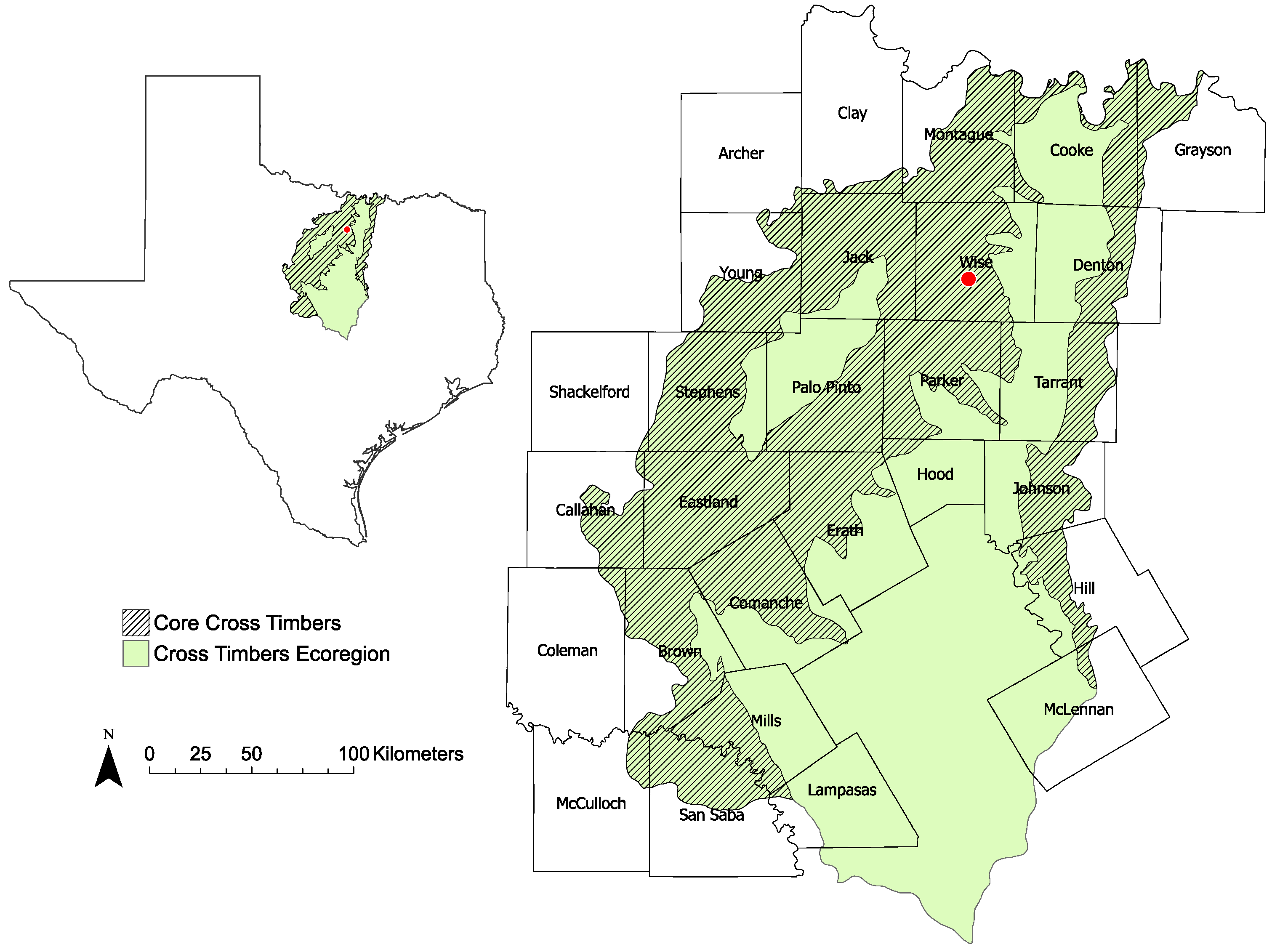
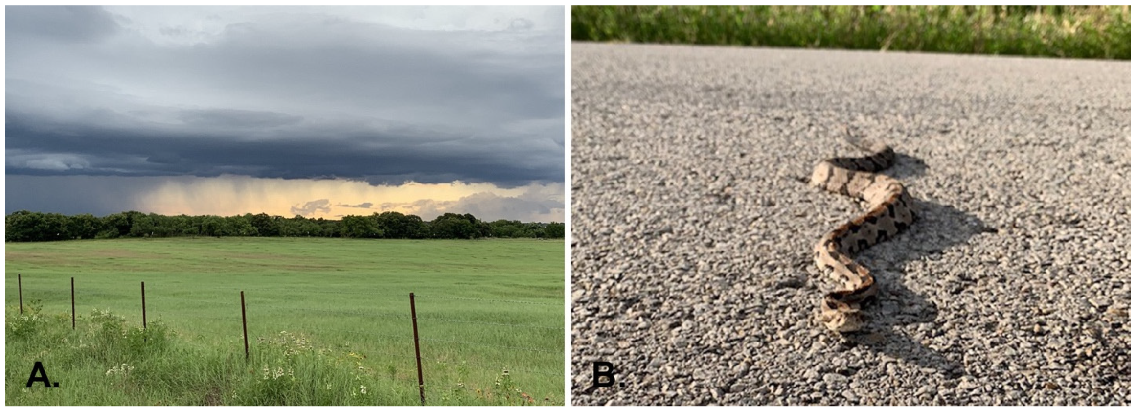
2.1. Study Area and Protocols

Our study area encompassed mostly oak woodlands interspersed with agricultural fields and riparian bottomlands southeast of Bridgeport, Wise County, Texas (Figure 1). This area is part of the western Cross Timbers ecoregion and has a humid subtropical climate with average July temperature of 28.9 °C and peak precipitation in late May [9]. Within our study area, we delineated three transects along county and farm-to-market roads for repeat-pass nocturnal road surveys. Transect A was a 14.3 km loop near the town of Cottondale, Texas, and included agricultural fields (primarily coastal Bermuda grass), riparian bottomland, and residential areas surrounding Cottonwood Creek, a minor tributary of the Trinity River. Transect B, near Paradise, Texas, extended for 7.1 km as a linear route, and from west to east included cultivated/grazed farmland, riparian bottomland along the West Fork of the Trinity River, disturbed mesquite scrub and residential development, and post oak woodland (Figure 2A). In addition to oaks, American elm, sugarberry, Texas ash, pecan, and cottonwood were prevalent along the transect. Transect C, a 9.9 km loop south of Bridgeport, represents the least disturbed transect, likely owing to large tracts of land owned by local farmers and cattlemen who have so far been unwilling to sell to developers. The transect includes hardwood forests (post oak, blackjack oak, American elm, and sugarberry), juniper groves on exposed limestone, rural residences, grazed cropland, riparian bottomland, and midgrass prairie. With respect to human activity, Transect A is the most developed, followed by Transect B and then Transect C. However, vehicular traffic is heavy and approximately equal on both Transect A and Transect B, and somewhat less on Transect C.
We performed surveys between the first week of April and the first week of October over three consecutive years, 2019–2021; the yearly range for surveys coincided with the normal activity season for nocturnal snakes in northern Texas. Nights for surveys were selected haphazardly and based primarily on the availability of observers; however, efforts were made to sample surveys over a wide variety of ambient conditions. We arranged transect order randomly for surveys and then repeated this randomization procedure over the length of each study season, which allowed us to ultimately survey each transect with similar intensity. In some instances, two or more transects were surveyed on the same night but always following our randomized order. We selected the following series of environmental covariates that have been associated with snake activity or purported to be associated with snake activity [10,11,12]: date (i.e., seasonal influence), ambient temperature, barometric pressure, humidity, wind speed, and lunar phase. We collected environmental data upon initiating and terminating surveys regardless of whether snakes were encountered, and we used the average value of these variables for analyses. We recorded start time and end time as well as number of replicate passes for each transect survey. Date was transformed to ordinal date using the %j format function in R base package and lunar phase was obtained using the lunar package [13]. For all snake observations, we identified species and recorded whether individuals were alive-on-road (AOR) or dead-on-road (DOR), as well as time, and location with GPS coordinates. For AOR snakes (including fatally wounded individuals), we collected surface temperature using an infrared thermometer. Snakes were identified by the same observer (CK) and recorded for positive identifications only (i.e., snakes that moved off roads before confident identification were not included). Occasionally, we collected DOR individuals in suitable condition to preserve as voucher specimens, which we deposited in the Amphibian and Reptile Diversity Research Center at the University of Texas at Arlington (Texas Parks and Wildlife Department permit SPR-0621-088). All data and metadata used for analyses are available in Table S1.

2.2. Statistical Analyses
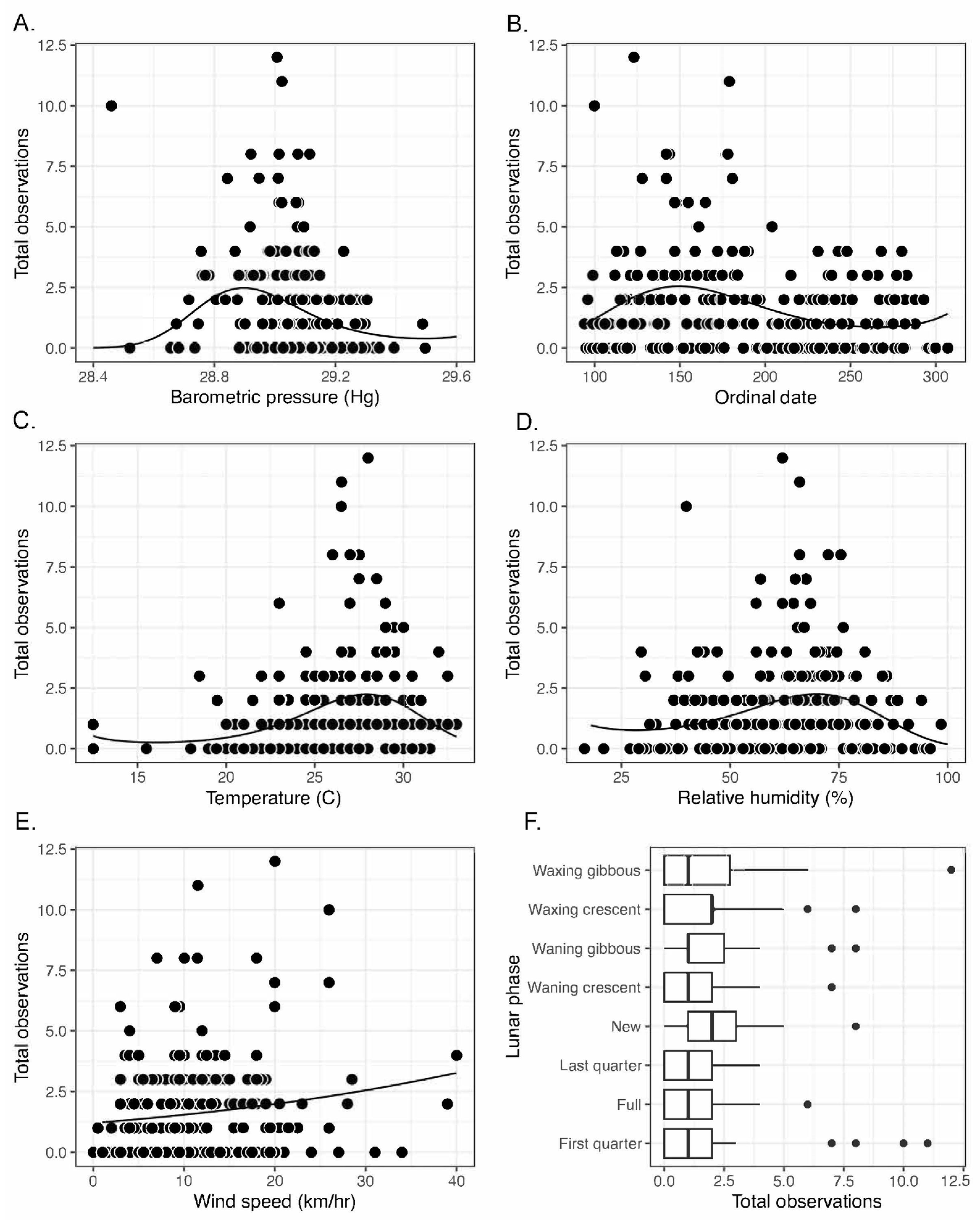
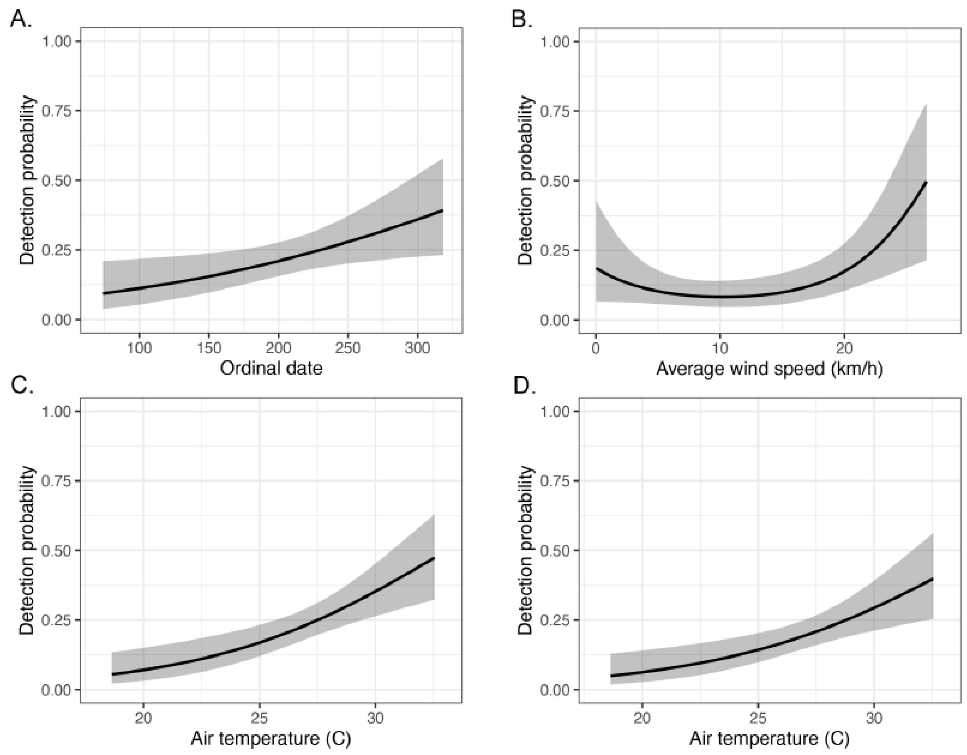
Upon completion of surveys, we summarized the cumulative counts of each species and their condition (AOR or DOR) across years for each of the three transects. For this study, we focused on activity patterns of the complete snake assemblage (i.e., all species combined) as well as for selected dominant species. We arbitrarily designated species as dominant when total encounters exceeded 30 individuals over the entire study period. For each of the dominant species, we first evaluated whether count frequencies differed across the three transects with goodness-of-fit (GoF) tests using R base package [14]. We used a chi-squared test of independence to determine whether frequencies of DOR and AOR snakes differed (i.e., were independent) across transects. We performed both tests using the R base function chisq.test(), with p-value obtained from 5000 data simulations. We evaluated covariates influencing activity patterns for all species combined (complete assemblage) using a series of generalized linear models (GLMs) with Poisson link functions. For these models, the response variable was total snake counts from individual surveys pooled across years and transects. Based on visual examination of data distributions and comparison of AICc values for competing models of polynomial functions, we modeled the influence of barometric pressure, ambient temperature, relative humidity, and ordinal date as third order polynomials (cubic), wind speed as first order (linear), and lunar phase as a factor with eight levels. Because of functional form complexity, we elected to model covariates separately. We evaluated model fit using AICc model selection and by calculating pseudo-R2 values for each model. Poisson GLMs were run using the glm() function in R base package, pseudo-R2 values obtained using nagelkerke() function from package rcompanion [15], and final models ranked using package AICcmodavg [16].
We further evaluated detection probabilities of dominant species as functions of the survey-specific covariates using site-occupancy models, which constitute a hierarchical framework that jointly estimates occurrence probability (psi) and detection probability (p) for each species using a repeat-survey metapopulation sampling design [17,18,19]. For occupancy models, the ecological state variable (i.e., occurrence) is often of primary interest and is corrected for by the detection submodel, which models the observation process as the complement of the false-negative error rate from repeat surveys. Given our relatively small study area, we assumed occupancy probability would likely be near 1.0 for most dominant species, and we were primarily interested in the estimates of detectability for these species and factors influencing them. We used a time-for-space substitution approach [8], in which we considered the repeated sets of surveys over each transect-year to be independent, and therefore our three transects were treated as nine separate transects for analyses. Species that are not detected from any transect-year combination will have lower occupancy estimates, which will increase p relative to assuming complete occupancy across species because p is conditional on psi. This feature of the model ensures that p is not calculated from sites or years where a species is presumably not present to be detected. The main assumptions for site-occupancy modeling [19], closure (no changes in occurrence state over course of study, or in this case, transect-years), no false positive errors, independence of detection, and homogeneity of detection probability, are likely not violated by the conditions of our study.
To prepare data for occupancy models, which incorporate a Bournoulli/Bournoulli distribution mixture, we summarized count data into detection–nondetection data frames as specified in Fiske and Chandler [20] and centered and scaled all continuous covariates. For each dominant species, we initially constructed two site-occupancy models: (1) a global detection model including all survey-specific covariates, and (2) a null model excluding the covariates. These models were compared with likelihood ratio tests and AICc values. If the global model was more informative than the null model, we evaluated which (if any) parameters were significant in determining variation in detection probabilities. To further explore potential functional relationships between environmental covariates and species detection, we performed additional models for covariates of interest from global models using linear and quadratic (second order polynomial) functions. The best-fit single-covariate models were used to estimate coefficients and produce prediction plots. We used null models for each of the species to estimate detection probability (and 95% CIs) because none of the covariates were influential in determining detection for many of the dominant species. We performed all site-occupancy models in the R package unmarked [20].

3. Results

Over the 3 yr period of study, we performed 250 repeat surveys of the three road transects, yielding a total of 406 snake observations of 16 species (Table 1). The number of surveys averaged 27.8 per transect for each field season (year) and collectively, the repeat surveys covered 19,358 total km (6969 for Transect A, 6834 for Transect B, and 5555 for Transect C). Overall, this yielded an encounter rate of 0.02 snakes per km surveyed. The total number of snakes observed across each of the transects was similar (Transect A = 132, Transect B = 144, and Transect C = 130). Seven species were each encountered more than 30 times and are considered dominant species for further analysis: three viperids (Agkistrodon laticinctus [n = 55], A. piscivorus [n = 35], and Crotalus horridus [n = 34]) and four colubrids (Nerodia erythrogaster [n = 39], N. rhombifer [n = 62], Pantherophis obsoletus [n = 74], and Thamnophis proximus [n = 59]) (Table 1). As expected, diurnal and semifossorial species were seldom encountered and were usually DOR. The remaining species are crepuscular/nocturnal but were observed with relatively low frequencies. Of the seven dominant species, only A. laticinctus and A. piscivorus differed significantly in frequency of counts across transects, with A. laticinctus having low apparent abundance in Transect B and A. piscivorus not detected from Transect A over the three years of surveys (Table 1). DOR snakes represented 35% of total observations, and independence of frequency of AOR to DOR snakes across the different transects was marginally significant with X2 = 5.393, simulated p-value = 0.067. Examination of observed and expected values indicated that Transect B had a slightly higher-than-expected frequency of DOR snakes, which was offset by a slightly lower than expected frequency of DOR snakes for Transect C (Table 2).
Results of model selection for Poisson GLMs of snake counts from individual surveys combined across species revealed that each covariate had significant, but only modest, effects on snake activity (Table 3, Figure 3). The best covariate for modeling snake count data was barometric pressure (pseudo-R2 = 0.26), which predicted highest snake activity at around 28.9 Hg, a value somewhat below the average barometric pressure of 29.1. For fitting this model, we excluded a single survey of 10 snake observations at 28.5 Hg from 4/10/2019, which was an obvious outlier for barometric pressure (outlier remains in Figure 3). This survey took place during high winds at the onset of a spring thunderstorm. Following barometric pressure, ordinal date and temperature both had pseudo-R2 values of 0.21 and differed by less than one AICc unit, indicating almost identical model fit. The GLM for ordinal date predicted peak activity at day 150, corresponding to late May, and the GLM for temperature predicted greatest activity at approximately 28 °C. Lunar phase had the lowest impact on snake activity, although slightly greater activity was observed during waning gibbous and new moon phases than during other periods of the lunar cycle.
Among the dominant species of the assemblage, detection probabilities were highest for Agkistrodon laticinctus, Pantherophis obsoletus, and Nerodia rhombifer, and lowest for Crotalus horridus and N. erythrogaster (Table 4). Null detection models fit as well as, or better than, global detection models for A. piscivorus and C. horridus, indicating that none of the measured covariates were important for influencing detection for either of these viperid species. Although the global model was a better fit than the null model for N. rhombifer, none of the covariates individually surpassed the alpha = 0.05 threshold for significance. For A. laticinctus, detection probability increased with ordinal date, suggesting greater activity on roads later in the field season (Figure 4). For both P. obsoletus and Thamnophis proximus, detection probability increased with ambient temperature (Figure 4), with increased confidence intervals after 28 °C, the peak activity for snakes as determined from Poisson GLMs. Finally, the global detection model for N. erythrogaster was a better fit than the null model, but only average wind speed was marginally significant. Upon further evaluation, we found average wind speed to conform better to a quadratic function, which provided significant covariate slope coefficients (Table 4). A prediction plot of the influence of average wind speed on detection for N. erythrogaster indicated an increase in detection above winds of 20 km/hr (Figure 4).

4. Discussion

In this study, we specified Poisson GLMs of survey count data to infer patterns of snake activity for all species combined and used the detection parameter from site-occupancy models as a proxy for estimating activity patterns for selected species. Despite pooling count data for all species for GLMs, we detected clear, but only moderate, signals of common responses to environmental covariates, particularly barometric pressure, ordinal date, and ambient temperature. Moreover, these responses were polynomial, indicating optimal values for activity (Figure 3). Snake activity peaked in late May, which also coincided with peak precipitation in the study area. This link between precipitation and date of peak activity also coincided with barometric pressure, for which snake activity peaked at lower-than-average values (lower barometric pressure is associated with onset of precipitation). Although seasonality of rainfall appears to drive patterns of activity for the assemblage overall, we did not evaluate precipitation directly, and humidity and wind speed (which peak during spring thundershowers) were of lesser importance. Taken together, these results suggest that periodicity of rainfall, but not necessarily precipitation itself, influences snake activity in the southern Cross Timbers. Precipitation as a primary predictor is consistent with many other studies of snakes, particularly from arid regions or where rainfall is seasonal [23,24,25]. Also consistent with previous work, snake activity was positively associated with ambient temperatures [11,12,26], and peaked at about 28 °C, above which there was a decline in predicted activity. Our finding that moon phase had small effect size was also expected in context of previous studies, as moon illumination has been shown to have modest and variable effects on snake activity and is confounded by various factors, including lunar precession and cloud cover [11,27,28].
Perhaps somewhat paradoxically, patterns at the assemblage level only partially corresponded to patterns for dominant species. For three of the seven dominant species (A. piscivorus, C. horridus, and N. rhombifer), none of the environmental covariates were effective for predicting activity on roads; for N. erythrogaster, average wind speed was the most important predictor despite wind speed showing only weak signal at the assemblage level; and for A. laticinctus, ordinal date was important, but the effect was opposite to the effect from the analogous GLM of the overall assemblage. With respect to ambient temperature, only two of the seven dominant species, P. obsoletus and T. proximus, responded similarly to activity patterns inferred from the entire assemblage. Importantly, barometric pressure, with the highest pseudo-R2 for GLMs, did not appear to influence detection appreciably for any of the dominant species evaluated separately.
Several reasons might contribute to the apparent discrepancy between assemblage and individual species analyses. First, as reported from previous studies of snake activity, responses to environmental covariates appear to be subtle [11,29], which compounds the general problem of weak inference that is related to observational studies generally [30]. The signal of covariate responses for the assemblage count dataset is based on the multitude of additive effects related to observations associated with all 406 individuals, which likely increases power over the fewer observations of the dominant taxa analyzed separately, at least for effects that are common across taxa. Furthermore, by collapsing count data into detection–nondetection data for site-occupancy modeling, we lost some available information related, for example, to potential multiple observations on survey nights under ideal conditions (however, cursory examination of multiple observations/night for species suggests effect sizes would likely also be small using analyses of count data). Ultimately, some environmental influences on activity will remain as unmodeled heterogeneity and some particularly subtle effects of measured covariates for dominant species will remain unexplained (e.g., the global model for N. rhombifer included humidity and ordinal date as marginally significant covariates, but these effects were not significant in simpler models including each covariate separately).
The predicted increases in detection for P. obsoletus and T. proximus with increases in ambient temperature were similar in slope, suggesting similar ambient thermal conditions for increased activity for these taxa. In this study, the mean surface temperature associated with AOR T. proximus (31.6 ± 1.2 °C) was significantly higher than for the other two natricine species (28.9 ± 0.89 °C for N. erythrogaster and 29.0 ± 1.13 °C for N. rhombifer; lm() function in R base statistics: F = 3.248, df = 2,99, p = 0.04), further supporting the relevance of warmer temperatures for activity in T. proximus relative to the water snakes. For N. erythrogaster, the increase in detection probability with increase in average wind speed might reflect pulses in dispersal immediately preceding warm-season thundershowers. Interestingly, neither humidity nor barometric pressure was inferred as significant in N. erythrogaster models, suggesting the possibility that wind conditions are a more important cue for movement in this species. Unlike for N. erythrogaster, we did not detect significant effects for any single covariate on N. rhombifer detection probability. Some evidence from other populations suggests that N. erythrogaster is more aquatic, or at least more specialized in habitat requirements, than is N. rhombifer [31], which could be consistent with a lack of covariate effects on activity for the latter species. The remaining dominant species with significant covariate effects was A. laticinctus, for which our models predicted increased activity later in the field season. Reasons for higher detectability later in the summer could relate to shifts toward increased nocturnality, possibly coinciding with seasonal variation in prey availability (see, e.g., [32]).
We detected significant differences in count frequencies across transects for only the two species of Agkistrodon, for which A. laticinctus was mostly absent from Transect B and A. piscivorus was not recorded from Transect A. The apparent low abundance of A. laticinctus from Transect B is consistent with additional years of informal survey by one of the authors (CK), but is difficult to explain given that, overall, the species had the highest detection probability of any species other than P. obsoletus (Table 4). In contrast, encounter frequency for A. piscivorus likely reflected the specific habitat requirement of perennial water sources [21,22], which were mostly absent from Transect A. Despite high levels of residential development, the dominant species of this study (excluding A. piscivorus) were encountered in Transect A with similar frequencies to the less developed transects. These species might have acclimated to residential habitat modification to some extent, which could provide improved prey abundances, alternative refugia (e.g., wood piles, greenhouses), and increased water availability during droughts.
Compared with similar studies, which often report DOR frequencies at over 70% (e.g., [33,34,35]), counts of DOR snakes were relatively low for our study at 35% of total observations. Presumably, studies vary in whether fatally wounded snakes are considered AOR or DOR, but how injured snakes are counted is rarely made explicit. We considered fatally wounded snakes as DOR for summary statistics, as studies focusing on mortality would likely categorize injured snakes as DOR. Frequencies of DOR snakes have been positively correlated with increased vehicular traffic in some, but not all, research [36,37,38], and from our study, relative frequency of DOR snakes was lowest on Transect C, which also had the lowest traffic. However, determining actual mortality rates from DOR percentages is problematic for various reasons [36,39], including behavioral avoidance of roads, at least by some taxa [40], variance in length of time for AOR and DOR snakes on roads, and the possibility that populations could already be decimated near high-traffic roadways before a study begins [39]. Despite problems with comparing DOR rates across studies and relating them to actual population mortality rates, it is apparent that road mortality and related habitat fragmentation from roads interrupt natural movement patterns and are likely detrimental to snake populations [33,40,41].
Of the dominant species from the study, T. proximus and C. horridus had the highest DOR frequencies at 44% each (Table 1). For T. proximus, we suggest that the apparent high DOR percentage relates to the greater diurnal activity of this species relative to other species, and that snakes killed from vehicle strikes during the day remained on roads into the evening hours during surveys. For C. horridus, the high percentage of DOR individuals could partly reflect the sluggish rectilinear locomotion coupled with conspicuous size and pattern against dark pavement at night, making individuals particularly vulnerable to vehicular mortality. Previous work on C. horridus has indicated possible population declines linked to road network densities [42] as well as behavioral avoidance of roads [43,44].
Our study provides one of the few assemblage-level assessments of snake communities in the southern Cross Timbers, and we documented a mix of species characteristic of either the southern Great Plains or eastern deciduous forests. At our study area, we generally observed prairie species less frequently than their woodland counterparts; for example, P. obsoletus was more frequently observed than was P. emoryi. Similarly, a notable aspect of our study was the relatively high frequency of encounter for C. horridus relative to C. atrox. The high relative abundance of C. horridus was unexpected given that our study location was at the extreme western edge of C. horridus but not the eastern edge of C. atrox distribution [5,21]. On a broad scale, the Cross Timbers of Texas, Oklahoma, and Kansas represents the western extent of C. horridus distribution, and our study area represents one of the westernmost verified counties for Texas. Regionally, the species is associated with hardwood bottomlands with ample fallen timber and greenbrier thickets, and accordingly, we recorded the highest counts of C. horridus from Transect B near the riparian corridor of the Trinity River (although this was not statistically significant). However, we have also observed timber rattlesnakes crossing roads in oak woodlands, upland prairies, and occasionally agricultural fields (Figure 2B), consistent with habitat use reported in a population-level study from the Oklahoma Cross Timbers [45]. Our data provide an important baseline for future studies evaluating successional changes in potentially competing snake species, including rattlesnakes (e.g., [46,47]). We previously documented hybridization between these narrowly sympatric congeners from the same county as our study area [48], and differences in relative abundances related to successional habitat changes can lead to unstable population dynamics and increased instances of hybridization [49,50].

5. Conclusions

The snake assemblage of the southern Cross Timbers consists mostly of natricine and colubrine colubrid, as well as crotaline viperid, species. We detected sixteen species over a 3 yr study of nocturnal snake activity patterns, and seven of the most frequently encountered species were included in both assemblage-level and individual analyses. Of the six environmental variables evaluated, barometric pressure was the most important in determining overall snake counts during surveys, followed closely by ordinal date and ambient temperature. Collectively, snakes were observed most frequently in late May under lower-than average barometric pressure, and warm ambient temperatures, corresponding to peak warm season precipitation. However, separate occupancy analyses of the dominant species revealed varied responses to environmental variables, with some seemingly not influenced significantly by any of the variables we examined. Together, these results suggest that patterns reflecting the overall snake assemblage are inconsistent at the level of individual species, which often show unique responses not reflected at the community level. Our results highlight the importance of evaluating activity patterns at different scales to provide a more comprehensive understanding of community temporal dynamics.

Supplementary Materials

The following supporting information can be downloaded at: https://www.mdpi.com/article/10.3390/d15090952/s1, Table S1: Excel file including datasheets and metadata used for this study.

Author Contributions

Conceptualization, C.K. and J.M.M.; methodology, C.K. and J.M.M.; formal analysis, J.M.M.; investigation, C.K.; data curation, C.K. and J.M.M.; writing—original draft preparation, C.K. and J.M.M.; writing—review and editing, C.K. and J.M.M. All authors have read and agreed to the published version of the manuscript.

Funding

This research was partly funded by the Tarleton State University College of Science and Mathematics “Banked Hours” research grant to J.M.M.

Institutional Review Board Statement

Because it did not alter natural snake behaviors, this study did not require institutional ethics approval (communication with Tarleton State University IACUC committee available upon request).

Data Availability Statement

All datasets used in this study have been made available as a Supplementary File.

Acknowledgments

We are grateful to A. King, Z. King, L. Woolam, D. Strom, K. Guay, and P. Hampton for field assistance and to B. Beverly for designing the map that appears as Figure 1.

Conflicts of Interest

The authors declare no conflict of interest. The funders had no role in the design of the study; in the collection, analyses, or interpretation of data; in the writing of the manuscript; or in the decision to publish the results.

References

  1. Francaviglia, R.V. The Cast Iron Forest: A Natural and Cultural History of the North American Cross Timbers; University of Texas Press: Austin, TX, USA, 1998. [Google Scholar]
  2. Hoagland, B.W.; Butler, I.H.; Johnson, F.L.; Glenn, S. The Cross Timbers. In Savannas, Barrens, and Rock Outcrop Plant Communities of North America; Anderson, R.C., Fralish, J.S., Baskin, J.M., Eds.; Cambridge University Press: Cambridge, UK, 1999; pp. 231–245. [Google Scholar]
  3. Therrell, M.D.; Stahle, D.W. A predictive model to locate ancient forests in the Cross Timbers of Osage County, Oklahoma. J. Biogeogr. 1998, 25, 847–854. [Google Scholar] [CrossRef]
  4. Ryberg, W.A.; Fitzgerald, L.A. Herpetofaunal inventory of Fort Wolters in north-central Texas. Southwest. Nat. 2005, 50, 267–272. [Google Scholar] [CrossRef]
  5. Dixon, J.R. Amphibians and Reptiles of Texas: With Keys, Taxonomic Synopses, Bibliography, and Distribution Maps, 3rd ed.; Texas A&M University Press: College Station, TX, USA, 2013. [Google Scholar]
  6. Sullivan, B.K. Long-term shifts in snake populations: A California site revisited. Biol. Conserv. 2000, 94, 321–325. [Google Scholar] [CrossRef]
  7. Owen, J.D.; Meik, J.M.; Schwertner, T.W. Preliminary nocturnal road survey of snakes in northeastern Swaziland: Effects of agriculture on relative abundance. Herpetol. Rev. 2015, 46, 12–15. [Google Scholar]
  8. Kéry, M.; Royle, J.A. Prelude and Static Models. In Applied Hierarchical Modeling in Ecology: Analysis of Distribution, Abundance and Species Richness in R and BUGS; Elsevier Academic Press: London, UK, 2016; Volume 1. [Google Scholar]
  9. U.S. Climate Data. Available online: usclimatedata.com (accessed on 1 April 2023).
  10. Daltry, J.C.; Ross, T.; Thorpe, R.S.; Wüsterm, W. Evidence that humidity influences snake activity patterns: A field study of the Malayan pit viper Calloselasma rhodostoma. Ecography 1998, 21, 25–34. [Google Scholar] [CrossRef]
  11. Eskew, E.A.; Todd, B.D. Too cold, too wet, too bright, or just right? Environmental predictors of snake movement and activity. Copeia 2017, 105, 584–591. [Google Scholar] [CrossRef]
  12. Schalk, C.M.; Weng, Y.H.; Adams, C.S.; Saenz, D. Spatiotemporal patterns of snake captures and activity in upland pine forests. Am. Midl. Nat. 2022, 187, 195–209. [Google Scholar] [CrossRef]
  13. Lazaridis, E. Lunar; Version 0.2-01; Lunar Phase and Distance, Seasons and Other Environmental Factors; 2022. [Google Scholar]
  14. R Core Team. R: A Language and Environment for Statistical Computing; R Foundation for Statistical Computing: Vienna, Austria, 2022; Available online: https://www.R-project.org/ (accessed on 31 October 2022).
  15. Mangiafico, S.S. Rcompanion; Version 2.4.30; Functions to Support Extension Education Program Evaluation; 2023. [Google Scholar]
  16. Mazerolle, M.J. AICcmodavg; Version 2.1-1; Model Selection and Multimodal Inference Based on (Q)AIC(c); 2017. [Google Scholar]
  17. MacKenzie, D.I.; Nichols, J.D.; Lachman, G.B.; Droege, S.; Royle, J.A.; Langtimm, C.A. Estimating site occupancy rates when detection probabilities are less than one. Ecology 2002, 83, 2248–2255. [Google Scholar] [CrossRef]
  18. Tyre, A.J.; Tenhumberg, B.; Field, S.A.; Niejalke, D.; Parris, K.; Possingham, H.P. Improving precision and reducing bias in biological surveys: Estimating false-negative error rates. Ecol. Appl. 2003, 13, 1790–1801. [Google Scholar] [CrossRef]
  19. MacKenzie, D.I.; Nichols, J.D.; Royle, J.A.; Pollock, K.H.; Bailey, L.L.; Hines, J.E. Occupancy Estimation and Modeling: Inferring Patterns and Dynamics of Species Occurrence; Elsevier: Amsterdam, The Netherlands, 2006. [Google Scholar]
  20. Fiske, I.; Chandler, R. unmarked: An R package for fitting hierarchical models of wildlife occurrence and abundance. J. Stat. Soft. 2011, 43, 1–23. [Google Scholar] [CrossRef]
  21. Werler, J.E.; Dixon, J.R. Texas Snakes: Identification, Distribution, and Natural History; University of Texas Press: Austin, TX, USA, 2000. [Google Scholar]
  22. Ernst, C.H.; Ernst, E.M. Snakes of the United States and Canada; Smithsonian Books: Washington, DC, USA, 2003. [Google Scholar]
  23. Bernardino, F.S.; Dalrymple, G.H. Seasonal activity and road mortality of the snakes of the Pa-hay-okee westlands of the Everglades National Park, USA. Biol. Conserv. 1992, 62, 71–75. [Google Scholar] [CrossRef]
  24. Marques, O.A.V.; Eterovic, A.; Endo, W. Seasonal activity of snakes in the Atlantic Forest in southeastern Brazil. Amphibia-Reptilia 2000, 22, 103–111. [Google Scholar] [CrossRef]
  25. McDonald, P.J. Snakes on roads: An arid Australian perspective. J. Arid Environ. 2012, 79, 116–119. [Google Scholar] [CrossRef]
  26. Sun, L.; Shine, R.; Debi, Z.; Zhengren, T. Biotic and abiotic influences on activity patterns of insular pit-vipers (Gloydius shedaoensis, Viperidae) from north-eastern China. Biol. Conserv. 2001, 97, 387–398. [Google Scholar] [CrossRef]
  27. Houston, D.; Shine, R. Movements and activity patterns of Arafura filesnakes (Serpentes: Acrochordidae) in tropical Australia. Herpetologica 1994, 50, 349–357. [Google Scholar]
  28. Sperry, J.H.; Ward, M.P.; Weatherhead, P.J. Effects of temperature, moon phase, and prey on nocturnal activity in ratsnakes: An automated telemetry study. J. Herpetol. 2013, 47, 105–111. [Google Scholar] [CrossRef]
  29. Brown, G.P.; Shine, R. Influence of weather conditions on activity of tropical snakes. Aust. Ecol. 2002, 57, 596–605. [Google Scholar] [CrossRef]
  30. Platt, J.R. Stong inference. Science 1964, 146, 347–353. [Google Scholar] [CrossRef]
  31. Laurent, E.J.; Kingsbury, B.A. Habitat separation among three species of water snakes in northwestern Kentucky. J. Herpetol. 2003, 37, 229–235. [Google Scholar] [CrossRef]
  32. Fitch, H.S. A Kansas Snake Community: Composition and Changes Over 50 Years; Krieger Publishing Company: Malabar, FL, USA, 1999. [Google Scholar]
  33. Rosen, P.C.; Lowe, C.H. Highway mortality of snakes in the Sonoran Desert of southern Arizona. Biol. Conserv. 1994, 68, 143–148. [Google Scholar] [CrossRef]
  34. Jochimsen, D.M.; Peterson, C.R.; Harmon, L.J. Influence of ecology and landscape on snake road mortality in a sagebrush-steppe ecosystem. Anim. Conserv. 2014, 17, 583–592. [Google Scholar] [CrossRef]
  35. Mccardle, L.D.; Fontenot, C.L., Jr.; Lutterschmidt, W.I. Demographic patterns of activity and road mortality from a long-term study of a wetland snake assemblage. Herpetol. Conserv. Biol. 2022, 17, 378–397. [Google Scholar]
  36. Andrews, K.M.; Gibbons, J.W.; Jochimsen, D.M. Ecological effects of roads on amphibians and reptiles: A literature review. In Urban Herpetology; Mitchell, J.C., Jung Brown, E., Bartholomew, B., Eds.; Society for the Study of Amphibians and Reptiles: Salt Lake City, UT, USA, 2008; Volume 3, pp. 121–143. [Google Scholar]
  37. Jones, T.R.; Babb, R.D.; Hensley, F.R.; LiWanPo, C.; Sullivan, B.K. Sonoran Desert snake communities at two sites: Concordance and effects of increased road traffic. Herpetol. Conserv. Biol. 2011, 6, 61–71. [Google Scholar]
  38. Croshaw, D.A.; Cassani, J.R.; Bacher, E.V.; Hancock, T.L.; Everham, E.M., III. Changes in snake abundance after 21 years in southwest Florida, USA. Herpetol. Conserv. Biol. 2019, 14, 31–40. [Google Scholar]
  39. Dodd, C.K., Jr.; Enge, K.M.; Stuart, J.M. Reptiles on highways in north-central Alabama, USA. J. Herpetol. 1989, 23, 197–200. [Google Scholar] [CrossRef]
  40. Paterson, J.E.; Baxter-Gilbert, J.; Beaudry, F.; Carstairs, S.; Chow-Fraser, P.; Edge, C.B.; Lentini, A.M.; Litzgus, J.D.; Markle, C.E.; McKeown, K.; et al. Road avoidance and its energetic consequences for reptiles. Ecol. Evol. 2019, 9, 9794–9803. [Google Scholar] [CrossRef]
  41. Wagner, R.B.; Brune, C.R.; Popescu, V.D. Snakes on a lane: Road type and edge habitat predict hotspots of snake road mortality. J. Nat. Conserv. 2021, 61, 125978. [Google Scholar] [CrossRef]
  42. Rudolph, D.C.; Burgdorf, S.J. Timber rattlesnakes and Louisiana pine snakes of the west gulf coastal plain: Hypotheses of decline. Texas J. Sci. 1997, 49, 111–122. [Google Scholar]
  43. Steen, D.A.; Smith, L.L.; Conner, L.M.; Brock, J.C.; Hoss, S.K. Habitat use of sympatric rattlesnake species within the Gulf Coast Plain. J. Wild. Manag. 2007, 71, 759–764. [Google Scholar] [CrossRef]
  44. Steen, D.A.; McClure, C.J.W.; Brock, J.C.; Rudolph, D.C.; Pierce, J.B.; Lee, J.R.; Humphries, W.J.; Gregory, B.B.; Sutton, W.B.; Smith, L.L.; et al. Landscape-level influences of terrestrial snake occupancy within the southeastern United States. Ecol. Appl. 2012, 22, 1084–1097. [Google Scholar] [CrossRef]
  45. Mohr, J.R.; Duvall, D. A prairie preference of the Oklahoma timber rattlesnake (Crotalus horridus) on the western fringe of its range. In Biology of Rattlesnakes II; Dreslik, M.J., Hayes, W.K., Beaupre, S.J., Eds.; ECO Herpetological Publishing and Distribution: Rodeo, NM, USA, 2017; pp. 136–141. [Google Scholar]
  46. Parker, W.S.; Brown, W.S. Species composition and population changes in two complexes of snake hibernacula in northern Utah. Herpetologica 1973, 29, 319–326. [Google Scholar]
  47. Mendelson, J.R., III; Jennings, W.B. Shifts in the relative abundance of snakes in a desert grassland. J. Herpetol. 1992, 26, 38–45. [Google Scholar] [CrossRef]
  48. Meik, J.M.; Fontenot, B.E.; Franklin, C.J.; King, C. Apparent natural hybridization between the rattlesnakes Crotalus atrox and C. horridus. Southwest. Nat. 2008, 53, 196–200. [Google Scholar] [CrossRef]
  49. Hasselman, D.J.; Argo, E.E.; McBride, M.C.; Bentzen, P.; Schultz, T.F.; Perez-Umphrey, A.A.; Palkovacs, E.P. Human disturbance causes the formation of a hybrid swarm between two naturally sympatric fish species. Mol. Ecol. 2014, 23, 1137–1152. [Google Scholar] [CrossRef]
  50. Grabenstein, K.C.; Taylor, S.A. Breaking barriers: Causes, consequences, and experimental utility of human-mediated hybridization. Trends Ecol. Evol. 2018, 33, 198–212. [Google Scholar] [CrossRef]
Figure 1. Map of Cross Timbers ecoregion in northcentral Texas showing the core Cross Timbers (with included counties), which historically consisted of oak woodlands and midgrass prairies, and the study area in Wise County (red symbol).
Diversity 15 00952 g001
Figure 2. Photographs depicting (A) the mosaic of pastoral fields (foreground) and oak woodland habitat typical of the study area along transect B, and (B) an adult timber rattlesnake (Crotalus horridus) crossing a section of Transect B.
Diversity 15 00952 g002
Figure 3. Number of snake observations per survey as a function of (A) barometric pressure, (B) ordinal date, (C) temperature, (D) relative humidity, (E) wind speed, and (F) lunar phase. Smoothers represent predicted values from best-fit GLMs with Poisson link functions.
Diversity 15 00952 g003
Figure 4. Detection probability plots for significant covariates estimated from occupancy analyses of individual species (with 95% CI in gray): (A) ordinal date for Agkistrodon laticinctus; (B) average wind speed for Nerodia erythrogaster; (C) air temperature for Pantherophis obsoletus; and (D) air temperature for Thamnophis proximus.
Diversity 15 00952 g004
Table 1. Cumulative counts of each snake species for each transect pooled across years, percent alive on road (AOR), predominate activity period (activity, compiled from [21,22]: D = diurnal; C = crepuscular; N = nocturnal), and, for each of the dominant species, results of goodness-of-fit (GoF) tests for differences in frequencies of counts across transects.
SpeciesTransects% AORActivityGoF Test
ABC
Agkistrodon laticinctus2413085DCNp = 0.0002
Agkistrodon piscivorus0231269DCNp = 0.0002
Coluber constrictor0100D
Coluber flagellum10233D
Crotalus atrox105100DCN
Crotalus horridus7171056DCNp = 0.092
Haldea striatula03125Semifossorial
Lampropeltis calligaster31180CN
Nerodia erythrogaster1417864DCNp = 0.201
Nerodia rhombifer29161766DCNp = 0.084
Opheodrys aestivus0530D
Pantherophis emoryi10583DCN
Pantherophis obsoletus24292164DCNp = 0.545
Pituophis catenifer20050DC
Storeria dekayi27469Semifossorial
Thamnophis proximus24241156DCNp = 0.060
Table 2. Frequencies of AOR (alive-on-road) and DOR (dead-on-road) snakes observed for each transect (pooled across years). Square brackets indicate expected values from a chi-squared test of independence (see text for details).
Transects
ABC
AOR84 [85.5]85 [93.3]95 [84.2]
DOR48[46.5]59 [50.7]36 [45.8]
Table 3. Model selection based on AICc for individual Poisson generalized linear models for environmental determinants of snake counts per survey (pooled across years and transects). All models were fit as third order polynomials except for wind speed (first order) and lunar phase (factor).
VariableKAICcΔAICcWeightLLPseudo-R2
Barometric pressure (Hg)4894.860.001−443.350.26
Ordinal date4933.5838.720−462.710.21
Air temperature (°C)4933.6938.830−462.760.21
Humidity (%)4943.1448.280−467.490.17
Wind speed (km/hr)2943.6448.780−469.790.16
Lunar phase8973.7978.930−478.600.10
Table 4. Results of site-occupancy models for evaluating detection probability (p) and environmental covariates associated with detection (i.e., activity) of dominant species from the study area. We evaluated detection probability for each species using null models (AICc N), and then compared null to global covariate models (AICc G) using likelihood ratio tests (chi-squared test statistic; LRT P). We further evaluated functional relationships of covariates significant from global models with separate models for each covariate (Coef. ± SE).
SpeciesAICc Np [95% CI]AICc GLRT PCovar.Coef. ± SE
A. laticinctus215.20.22 [0.17, 0.28]208.70.002ord date0.51 ± 0.21
A. piscivorus167.10.16 [0.12, 0.23]166.90.019
C. horridus183.40.12 [0.08, 0.16]189.60.120
N. erythrogaster187.50.12 [0.09, 0.17]183.80.006wind0.13 ± 0.21
wind20.39 ± 0.17
N. rhombifer235.40.21 [0.16, 0.27]232.30.007
P. obsoletus270.00.22 [0.18, 0.28]261.90.001temp0.68 ± 0.19
T. proximus245.70.19 [0.14, 0.24]238.40.002temp0.63 ± 0.20
Disclaimer/Publisher’s Note: The statements, opinions and data contained in all publications are solely those of the individual author(s) and contributor(s) and not of MDPI and/or the editor(s). MDPI and/or the editor(s) disclaim responsibility for any injury to people or property resulting from any ideas, methods, instructions or products referred to in the content.

