Pan-Atlantic Comparison of Deep-Sea Macro- and Megabenthos

Abstract

Deep-sea benthic fauna is vital for a well-functioning marine ecosystem but is increasingly under threat from a changing environment. To monitor and conserve this fauna, an understanding of their large-scale spatial and bathymetric distribution and their environmental drivers is necessary. In this study, we conduct a multivariate analysis on abundance benthic fauna data collected at the phylum and multitaxon levels using an epibenthic sledge (EBS) across the Atlantic, and identify the environmental factors that affect such data. Our findings show a decrease in abundance with depth in most of the Atlantic but find relatively heterogeneous abundances with depth within the Southern Ocean. Principal component analyses indicate differences in environmental conditions south of the Antarctic Polar Front (~52° S), outlining contrasts in the quantities of macronutrients and physical factors. Despite this, community composition seemed markedly similar throughout the Atlantic with the Antarctic Circumpolar Current seemingly not affecting benthic community composition for higher taxonomic levels. Those differences that did occur were largely caused by benthic chlorophyll, benthic iron, and surface silicate through a Bio-ENV. Overall, we argue that further large-scale spatial and bathymetric distribution studies are important amid environmental changes that are driving shifts in benthic community abundance and composition.

1. Introduction

Benthic marine life performs an important role in the overall function of marine ecosystems e.g., [1,2,3]. Benthic fauna may contribute towards the transformation and transport of organic matter, the transport of oxygen, nutrient cycling, and secondary production [4,5,6,7]. Benthic fauna can also be important in the provision of habitats e.g., [8,9,10] or in altering local physiochemical conditions [11], topography [12], or sediment availability through the bioturbation of sediments [11]. As different taxa perform different roles in the maintenance and regulation of ecological processes, a diverse benthic fauna is widely considered to positively impact upon ecosystem stability and function [13,14].

Benthic fauna is vulnerable to changes in the physical and chemical properties of the water column. These changes can be caused directly or indirectly by human activities. For example, direct impacts include fisheries [15,16,17] and future mining for seabed minerals, which scour the seafloor and disturb important habitats, as e.g., reviewed by [18]. Indirect impacts can include those caused by anthropogenically induced climate change, which may lead to increasing sea temperatures, ocean acidification, and changes in ocean currents, amongst other changes [19]. Additionally, natural disturbances such as volcanoes, hydrothermal vents, or turbidite events can also alter benthic habitats and their communities [20,21,22]. These long-lasting modifications can threaten habitats necessary to species survival and lead to shifts in the distribution of species e.g., [23,24,25]. Changes in environmental conditions may therefore result in an irreversible loss of biodiversity.

As the largest biome on Earth, an understanding of the deep sea (>200 m) now is critical for evaluating shifts in their biodiversity patterns caused by environmental changes in the near future. However, this understanding is inhibited by the comparatively limited data, owing to the cost and time of sampling. More recently, sampling activity in the Atlantic has increased in an effort to identify benthic biodiversity and elucidate deep-sea ecosystems e.g., [26,27,28,29,30,31,32,33,34,35,36,37,38,39,40,41]. The Atlantic Ocean is considered a particularly interesting study area, as deep-sea geological features including the Mid-Atlantic Ridge and Greenland-Iceland-Faroe Ridge are believed to form barriers to benthic species migration e.g., [29,42,43]. Additionally, ocean currents including the Antarctic Circumpolar Current are suggested to influence species distribution in Antarctic waters e.g., [44], whilst the Atlantic Meridional Overturning Circulation (AMOC) dictates the regional environmental characteristics, such as salinity and temperature, throughout large parts of the Atlantic Ocean [45].

Recent investigations have focused on the relationship between deep-sea biodiversity patterns and environmental characteristics, such as depth, temperature, salinity, and nutrient availability, amongst others e.g., [28,31,46,47,48,49,50]. This includes studies that have attempted to unravel benthic biodiversity patterns within regions of the Atlantic e.g., [28,47]. For example, Kaiser et al. [28] found that benthic macrofauna density in the South Atlantic abyss is probably linked to food availability. In the Atlantic sector of the Southern Ocean, Di Franco et al. [47] identified depth as the main driver in shaping peracarid assemblages, while Stransky et al. [51,52] identified sediment characteristics off Greenland as important, as did Frutos et al. [53] in the southern Bay of Biscay. However, statistical analyses of benthic biodiversity patterns and abiotic variables encompassing the wider Atlantic Ocean have hitherto been limited.

Understanding the benthic spatial and bathymetric distributions and how these biodiversity patterns are influenced by abiotic variables is the basis for future monitoring and conservation efforts. In this study, we analyze Pan-Atlantic benthic data from a range (119–8338 m) of depths. This was compiled from published [28,54,55,56,57,58,59,60] and unpublished data from samples collected using an epibenthic sledge (EBS). The objectives of this study were to: (1) examine large-scale spatial and depth-related patterns of the Atlantic macro- and megabenthos, (2) assess abundance of the benthic fauna at the phylum and multitaxon levels (class or order level), and (3) identify environmental variables influencing these patterns.

2. Materials and Methods

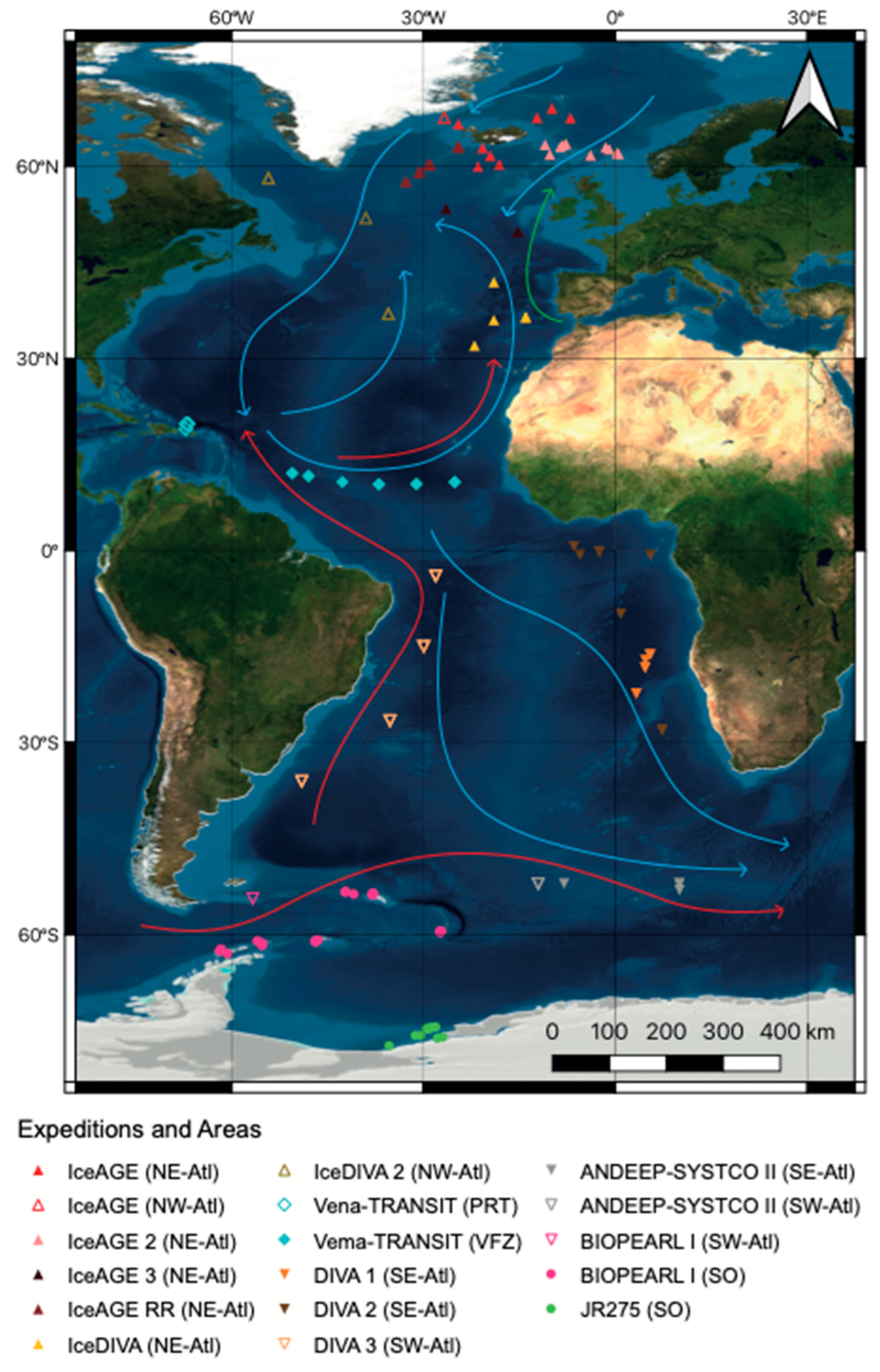
Comparable deep-sea benthos data were collected using an EBS with an epi- and a suprabenthic net in the Atlantic Ocean since 2006 during the international research expeditions ANDEEP-SYSTCO II (Antarctic benthic deep-sea biodiversity, colonization history, and recent community patterns–system coupling), BIOPEARL I (biodiversity dynamics: phylogeography, evolution, and radiation of life), DIVA 1–3 (latitudinal gradients of deep-sea biodiversity in the Atlantic), IceAGE 1–3 (Icelandic marine animals: genetic and ecology) and RR (Icelandic marine animals: genetic and ecology Reykjanes Ridge), IceDIVA (Icelandic marine animals meet diversity along latitudinal gradients in the deep sea of the Atlantic Ocean), IceDIVA 2 JR275 and Vema-TRANSIT (bathymetry of the Vema fracture zone and Puerto Rico trench and abyssal Atlantic biodiversity study) (Table 1, Figure 1). While EBS data at high taxon level were published for ANDEEP-SYSTCO II, DIVA1-3 and Vema-TRANSIT [26,28,56], unpublished data for BIOPEARL I, IceAGE1-3 and RR, IceDIVA, IceDIVA 2, and JR275 was acquired from the German Centre of Marine Biodiversity (DZMB) Senckenberg and British Antarctic Survey [61]. Each of these expeditions used a standardized sampling protocol.

Table 1. Technical information of expeditions (South Atl = South Atlantic, SO = Southern Ocean, North Atl = North Atlantic, VFZ = Vema fracture zone, PRT = Puerto Rico trench).

Project	Cruise Number	Date	Vessel	Sample Area	Reference
ANDEEP-SYSTCO II	ANT-XXVIII/3	7 January 2012– 11 March 2012	Polarstern	South Atl	[26]
BIOPEARL I	JR 144	26 February 2006–17 April 2006	RRS James Clark Ross	SO	[62]
DIVA 1	M48/1	6 July 2000– 02 August2000	RV Meteor	South Atl	[32]
DIVA 2	M63/2	26 February 2005– 31 March 2005	RV Meteor	South Atl	[41]
DIVA 3	M79/1	10 June 2009– 26 August2009	RV Meteor	South Atl	[33]
IceAGE	M85/3	27 August 2011–28 September 2011	RV Meteor	North Atl	[34]
IceAGE 2	POS456	20 July 2013– 4 August 2013	RV Poseidon	North Atl	[40]
IceAGE RR	MSM75	29 June 2018– 8 September 2018	RV Ms Merian	North Atl	[37]
IceAGE 3	SO276 (MerMet17-06)	22 June 2020– 26 July2020	RV Sonne	North Atl	[35]
IceDIVA	SO280	8 January 2021– 7 February 2021	RV Sonne	North Atl	[63]
IceDIVA 2	S0286	5 November 2021– 8 December 2021	RV Sonne	North Atl	[38]
JR275	JR275	7 February 2012– 2 March 2012	RRS James Clark Ross	SO, South Atl	[39]
Vema-TRANSIT	SO237	14 December 2014–26 January 2015	RV Sonne	VFZ, PRT	[64]

Table 1. Technical information of expeditions (South Atl = South Atlantic, SO = Southern Ocean, North Atl = North Atlantic, VFZ = Vema fracture zone, PRT = Puerto Rico trench).

Project	Cruise Number	Date	Vessel	Sample Area	Reference
ANDEEP-SYSTCO II	ANT-XXVIII/3	7 January 2012– 11 March 2012	Polarstern	South Atl	[26]
BIOPEARL I	JR 144	26 February 2006–17 April 2006	RRS James Clark Ross	SO	[62]
DIVA 1	M48/1	6 July 2000– 02 August2000	RV Meteor	South Atl	[32]
DIVA 2	M63/2	26 February 2005– 31 March 2005	RV Meteor	South Atl	[41]
DIVA 3	M79/1	10 June 2009– 26 August2009	RV Meteor	South Atl	[33]
IceAGE	M85/3	27 August 2011–28 September 2011	RV Meteor	North Atl	[34]
IceAGE 2	POS456	20 July 2013– 4 August 2013	RV Poseidon	North Atl	[40]
IceAGE RR	MSM75	29 June 2018– 8 September 2018	RV Ms Merian	North Atl	[37]
IceAGE 3	SO276 (MerMet17-06)	22 June 2020– 26 July2020	RV Sonne	North Atl	[35]
IceDIVA	SO280	8 January 2021– 7 February 2021	RV Sonne	North Atl	[63]
IceDIVA 2	S0286	5 November 2021– 8 December 2021	RV Sonne	North Atl	[38]
JR275	JR275	7 February 2012– 2 March 2012	RRS James Clark Ross	SO, South Atl	[39]
Vema-TRANSIT	SO237	14 December 2014–26 January 2015	RV Sonne	VFZ, PRT	[64]

Figure 1. Map of the Atlantic Ocean showing EBS deployment locations from 13 expeditions with each symbol marking a sampling event. Red arrows indicate the major Antarctic bottom water deep-sea currents and blue arrows indicate Arctic bottom water deep-sea currents. Green arrow indicates bottom currents of common water (current scheme modified after Stow et al. [65]). (SO = Southern Ocean, SE Atl = southeast Atlantic, SW Atl = southwest Atlantic, VFZ = Vema fracture zone, PRT = Puerto Rico trench, NE-Atl = northeast Atlantic, NW = northwest Atlantic).

Figure 1. Map of the Atlantic Ocean showing EBS deployment locations from 13 expeditions with each symbol marking a sampling event. Red arrows indicate the major Antarctic bottom water deep-sea currents and blue arrows indicate Arctic bottom water deep-sea currents. Green arrow indicates bottom currents of common water (current scheme modified after Stow et al. [65]). (SO = Southern Ocean, SE Atl = southeast Atlantic, SW Atl = southwest Atlantic, VFZ = Vema fracture zone, PRT = Puerto Rico trench, NE-Atl = northeast Atlantic, NW = northwest Atlantic).

For the analysis, we defined seven regions to group EBS deployment locations. Four of these regions were prescribed based on their position relative to the Equator and the mid-Atlantic Ridge (MAR): northeast, northwest, southeast, and southwest Atlantic. Additional regions include the Vema fracture zone as a gap in the MAR, the Puerto Rico trench as a deep-sea trench, and the Southern Ocean south of the MAR. The sampling depth ranged from 119 m to 8338 m and included non-deep-sea stations if available for comparison reasons. As the sampling depth spanned over 8000 m, we grouped depth into depth zones: (1) shelf defined as 0 to 200 m for all areas, except the Southern Ocean, where it was defined as 0 m to 500 m due to continental depression caused by the weight of the ice sheet [66]; (2) upper slope as 200/500 m to 1000 m [66,67,68]; (3) lower slope as 1000 m to 3000 m [68]; (4) abyssal as 3000 m to 6000 m [68]; and (5) hadal as larger than 6000 m [69]. For different parts of the analysis, we used the regional and depth groups independent from one another while combining these groupings for others.

2.1. Sampling and Sample Processing

In total, data for 143 EBS deployments—referred to as stations from here on—from 13 expeditions were available for analyses based on identification on 50 taxon levels, including phyla, subphyla, classes, and orders [61]. During all expeditions, an EBS with an epi- and a suprabenthic net following the sizes and height defined by Brandt et al. [70] and Brenke [71] were used, enabling comparability of samples. This type of EBS was a suitable device for sampling small benthic fauna on and above the seabed, including macrofauna and small-sized megafauna. Macrofauna were defined as invertebrate organisms of a size range from 300 µm to 2 cm in size, while invertebrates larger than 2 cm in size are referred to as megafauna [72]. Each of the nets had an opening of 100 × 33 cm and net mesh size of 500 μm. The cod ends were equipped with net-buckets containing 300-μm mesh windows. On standard deployments, cable lengths that were 1.5 times longer than the water depth were laid out, with the EBS then trawled with 1 kn for 10 min on the seabed. Trawling times and cable length were shortened where required by the seafloor topography and were implemented in the haul distance calculation. Once on the deck, the content of the samplers was fixed in 96% undenaturated and pre-cooled (at −20 °C) ethanol or 4% buffered formalin. If required because of extensive collected sediment, the sampler content was sieved through 300-µm test sieves to remove mud and silt. The haul distances were calculated based on equation (4) in Brenke [61,71]. For comparison between stations, abundance data were standardized to a 1000 m² trawled seabed area.

After at least 48 h of fixation, samples from the epi- and suprabenthic net were sorted under stereomicroscopes into the lowest possible higher taxon level (phylum to order) and counted to determine abundance. Abundance counts per taxon from the epi- and suprabenthic nets were pooled following Brenke [55]. Annelida and Arthropoda were only counted if the head was present; Ophiuroidea only if the disc was present; brachiopod, molluscan, and ostracod shells were checked for soft tissues; only intact, small-sized sponges were counted, not broken sponge tissues, which occurred in samples from the southern Weddell Sea.

In this study, we included data for 41 higher taxa of the initially separated 50 taxa ranging from phyla to orders. Any classes and orders are from herein referred to together as “Multitaxa”. We excluded Foraminifera and Bryozoa due to difficulties in distinguishing whole individuals from broken pieces, as well as the subphylum vertebrata as it was outside the scope of this study. Brachiopoda, Chaetognatha, Echiura, Hemichordata, Nematoda, Nemertea, Phoronida, Platyhelminthes, Porifera, and Priapulida were not identified beyond the phylum level and subclass level for the Echiura. Other Annelida were separated into Polychaeta, Sipuncula, Oligochaeta, and Hirudinea. The phylum Arthropoda was split into the subphylum Chelicerata and Crustacea, with the former comprising Pycnogonida and Acarina and the latter comprising crustacean order levels. Chordata only consisted of Tunicates. Echinodermata and Mollusca were separated into classes. For the DIVA 1 and 2 data sets, Cnidaria and Echinodermata were not further discriminated into classes. For the DIVA 1, IceAGE 1-3, and RR, and IceDIVA and IceDIVA 2 data sets, Aplacophora were not separated into Caudofoveata and Solenogastres. So, if corresponding data on class assignment were available, these were reported separately, but for all univariate and multivariate analyses, classes within Aplacophora, Cnidaria, and Echinodermata were grouped within their phyla.

2.2. Environmental Data

The environmental parameters for this study were provided by Bio-ORACLE http://www.bio-oracle.org/ (accessed on 6 January 2023); Bio-ORACLE identifies average (mean) values for different physical and chemical variables over a 14-year time period from 2000–2014 through a combination of satellite and in situ measurements at a spatial resolution of 5 arcmine.g., [47,73,74,75,76,77]. For this study, Bio-ORACLE data for the surface measurements for salinity (PSS), silicate (mol/m³), iron (mmol/m³; mol/m³), phosphate (mmol/m³; mol/m³), nitrate (mmol/m³; mol/m³), chlorophyll-a (mg/m³; mg/cm³), primary production (g/m³/day), and calcite (mol/m³) were included [73]. Furthermore, benthic data (maximum depth) for salinity (PSS), silicate (mol/m³), iron (mmol/m³; mol/m³), phosphate (mmol/m³; mol/m³), nitrate (mmol/m³; mol/m³), chlorophyll-a (mg/m³; mg/cm³), primary production (g/m³/day), temperature (°C), and current velocity (m/s) were included from Bio-ORACLE as well [73].

2.3. Statistical Analyses

The univariate and multivariate analyses were conducted for two higher taxonomic levels, one including phyla and two arthropod subphyla only, and the other including the 41 higher taxa mentioned above. The motivation for using the two arthropod subphyla was the high abundance of the crustacea in the benthic deep sea e.g., [59,78]. To assess the patterns in taxon richness, specimen abundances, biodiversity, and community structure of the macro- and megabenthic fauna, the data were processed using Microsoft Excel 16.69.1 [79], and univariate as well as multivariate analyses were performed with PRIMER v6.0 [80]. Raw data (taxon identification and abundance) were first organized into a double entry taxon–station matrix with standardized data expressed as taxon individuals per 1000 m². These faunal densities were reported to the nearest integer. The taxon density station matrix was further converted by grouping stations from the same depth range and regions. This enabled density and relative abundance results to be analyzed at an individual and regional scale.

Before conducting any further statistical analyses with PRIMER v6.0 [80], the macro- and megabenthic community data at the phylum and multitaxon levels were fourth-root transformed. This was performed to mitigate the impact of any outliers which are likely present in such a diverse and large dataset with a large range of abundance values. This fourth-root transformed dataset was used in all of the following statistical tests. To identify and visualize the level of similarities between density data at the phylum and multitaxon levels, non-metric multidimensional scaling (nMDS) was performed with combined depth region groups. The Bray–Curtis dissimilarity coefficient was applied to non-transformed and fourth-root transformed density data of the phylum and multitaxon level data to obtain similarity matrices using PRIMER v6.0 [73]. Hierarchical clustering with group-averaged linking and non-metric multidimensional scaling (nMDS) was then performed using these matrixes. This was followed by one-way ANOSIM tests to investigate the differences in community composition between groups of stations. For the ANOSIM tests, stations were grouped independently into depth and region zones. A similarity percentages routine (SIMPER) was run on the region and depth zone groups [80] to understand intra-group similarities and inter-group dissimilarities. The cut-off for contributing species was applied (50%) to the SIMPER analysis using combined depth region groups. In order to characterize the environmental variables for the stations, a principal components analysis (PCA) containing all 21 abiotic environmental variables was performed. The environmental data were normalized prior to conducting the PCA. Lastly, a BIO-ENV (BEST) analysis was carried out to determine the abiotic environmental variables driving the community patterns at the station level. For this, environmental data were normalized and categorized using Euclidean similarities. For the BIO-ENV (BEST), a Spearman rank correlation was used.

3. Results

For this study, a total of 495,893 specimens were included from 143 EBS stations and assigned into seven regions [61]. The regions were divided into depth zones, resulting in two shelf, three upper slope, three lower slope, five abyssal, and one hadal regional depth zone groupings. The sampled macrofauna used in this study included 16 phyla and 41 higher taxa of which 6 phyla and 17 higher taxa were dominant while the others were infrequent (Figure 2).

Standardized absolute abundance (Ind./1000 m²) varied between stations, ranging from 6 to 49,105 individuals, with stations located in the northeastern Atlantic upper slope, Southern Ocean shelf, and upper slope showing the highest macrofaunal abundance. Stations in the southwestern Atlantic shelf, southwestern Atlantic, and hadal Puerto Rico trench had the lowest abundance. On average, between 163 and 12,987 individuals were sampled per 1000 m² per region (Figure 3 and Figure 4) [61]. In most regions, abundance declined with depth. However, this was less apparent for the Southern Ocean, where upper slope stations (238–34,483 Ind./1000 m²) showed a generally higher abundance than shelf stations (49–42,459 Ind./1000 m², Figure 4).

Samples were dominated by the phylum Arthropoda, with 14.4–72.8% in relative abundance. This was followed by Annelida with 7.7–32.9%, Mollusca with 4.6–24.1%, and Echinodermata with 0.4–20.2%. The least dominant phyla were Porifera (0–32.7%), Nematoda (0.1–11.3%), and others (0–2.1%) (Figure 5a). When compared at the multitaxa level, the most abundant multitaxa were the order Isopoda, with 5.4–55.8%, followed by the classes Polychaeta with 11.4–29.8%, Ophiuroidea with 0–28.6%, and Gastropoda with 0.2–22.9%. Among the least abundant taxa were the phylum Chaetognatha (0–1.7%) and the classes Scaphopoda (0–1.8%) and Pycnogonida (0–2%) (Figure 5b).

Notably, stations in the hadal Puerto Rico trench showed a strong difference in relative abundance composition. This was mainly driven by high percentages of Isopoda and Holothuroidea appearing simultaneously with low percentages of Cumacea. In addition, fauna of the southwestern Atlantic shelf strongly differed, which was mainly caused by high percentages of Ophiuroidea and Gastropoda in combination with low percentages of isopods. Remarkably, Copepoda and Cumacea were not present in this area at all (Figure 5b).

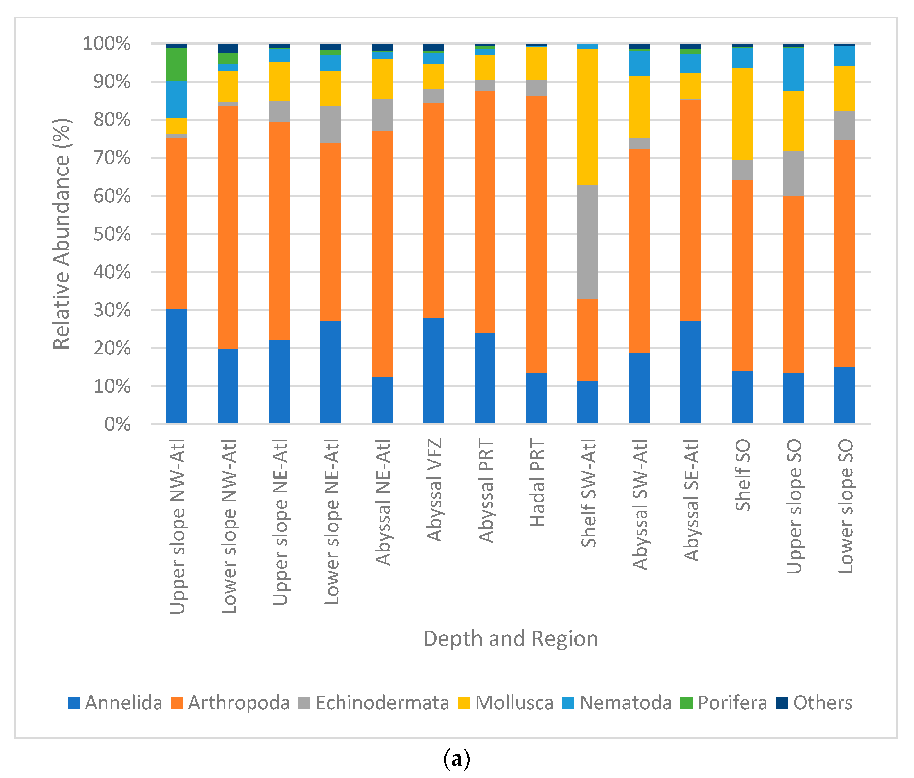
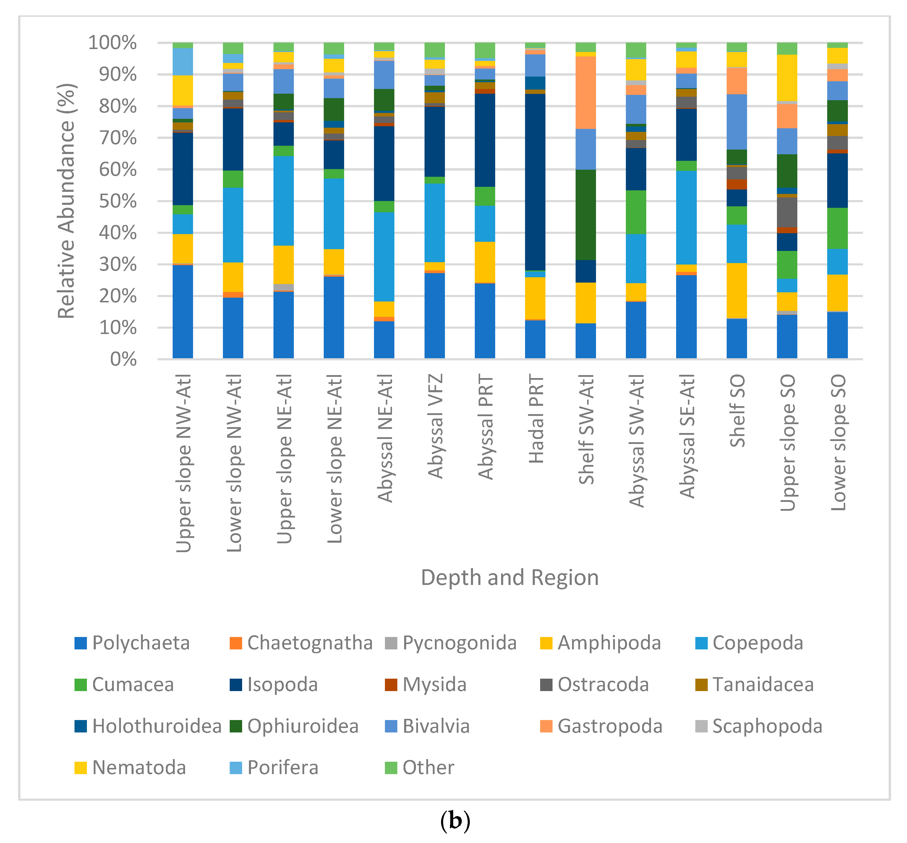
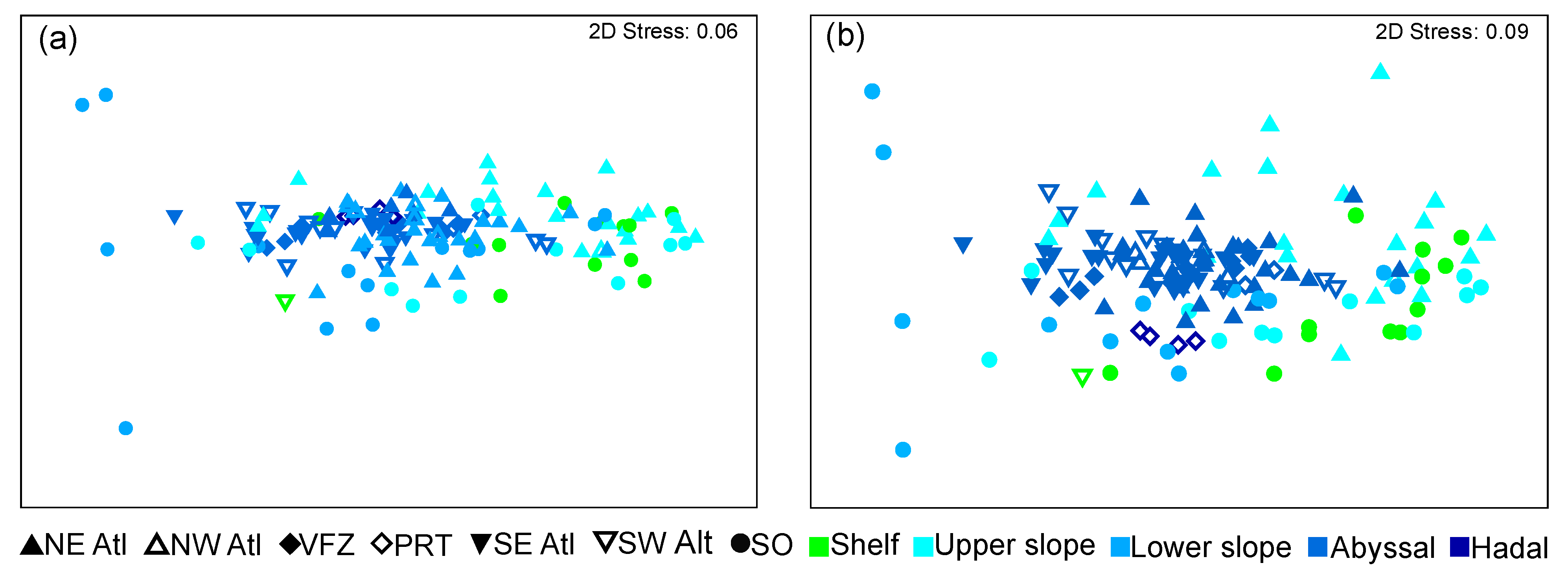
Macro- and Mega Fauna Composition

Non-metric multidimensional scaling (nMDS) provided similar results for the phyla and taxa analyses, with no clear groups of depth and region categories being formed (Figure 6).

Results from the nMDS largely matched findings from the analysis of similarities (ANOSIM) and showed generally little differences between groups at both taxonomic levels. Differences that were observed in the ANOSIM (

Table 2. One-way ANOSIM for depth at the phylum level. Statistically significant (p value = 0.05) values printed in bold. ANOSIMs performed with 4th-root transformation: Significance level of sample statistic: 0.1%; number of permutations: 999 (Random sample from a large number) and number of permuted statistics greater than or equal to Global R: 0. (SO = Southern Ocean, SE Atl = southeast Atlantic, SW Atl = southwest Atlantic, VFZ = Vema fracture Zone, PRT = Puerto Rico trench, NE Atl = northeast Atlantic, NW = northwest Atlantic).

Depth (Phylum)		Global R: 0.264
Groups	RStatistic	Significance Level (%)
Abyssal, Hadal	0.035	37.8
Abyssal, Shelf	0.591	0.1
Abyssal, Lower Slope	0.143	0.1
Abyssal, Upper Slope	0.476	0.1
Hadal, Shelf	0.35	0.9
Hadal, Lower Slope	0.077	27.2
Hadal, Upper Slope	0.186	10.4
Shelf, Lower Slope	0.209	0.7
Shelf, Upper Slope	–0.062	81.8
Bathyal, Slope	0.146	0.1

and

Table 3. One-way ANOSIM for depth at the multitaxa level. Statistically significant (p value = 0.05) values printed in bold. ANOSIMs performed with 4th-root transformation: Significance level of sample statistic: 0.1%; number of permutations: 999 (Random sample from a large number) and number of permuted statistics greater than or equal to Global R: 0. (SO = Southern Ocean, SE Atl = southeast Atlantic, SW Atl = southwest Atlantic, VFZ = Vema fracture Zone, PRT = Puerto Rico trench, NE Atl = northeast Atlantic, NW = northwest Atlantic).

Depth (Multitaxa)		Global R: 0.321
Groups	R Statistic	Significance Level (%)
Abyssal, Hadal	0.545	0.2
Abyssal, Shelf	0.715	0.1
Abyssal, Lower Slope	0.196	0.1
Abyssal, Upper Slope	0.501	0.1
Hadal, Shelf	0.528	0.3
Hadal, Lower Slope	0.308	5.5
Hadal, Upper Slope	0.356	1.4
Shelf, Lower Slope	0.256	0.8
Shelf, Upper Slope	–0.026	58.5
Bathyal, Slope	0.13	0.2

) were largely present between groups of different depths. In general, any differences between groups were less pronounced at the phyla level than at the multitaxon level. The greatest difference between groups was seen between the abyssal and shelf/upper slope stations (R value: 0.476–0.715). In addition, the hadal stations differed to the shelf, upper slope, and abyssal stations (R value: 0.35–0.545). However, it must be noted that the hadal stations were only present from one region (the Puerto Rico trench) in the analysis. Lastly, the lower slope stations were relatively similar to the shelf, upper slope, and abyssal stations (R value: 0.13–0.256).

The ANOSIM was conducted to analyze similarities between different regions (the global R value at the phyla level was 0.264 and at the multitaxon level 0.32;

Table 4. One-way ANOSIM for regions at the phylum level. Statistically significant (p value = 0.05) values printed in bold. ANOSIMs performed with 4th-root transformation: Significance level of sample statistic: 0.1%; number of permutations: 999 (Random sample from a large number) and number of permuted statistics greater than or equal to Global R: 0. (SO = Southern Ocean, SE Atl = southeast Atlantic, SW Atl = southwest Atlantic, VFZ = Vema fracture Zone, PRT = Puerto Rico trench, NE Atl = northeast Atlantic, NW = northwest Atlantic).

Regions (Phylum)		Global R: 0.111
Groups	R Statistic	Significance Level (%)
VFZ, PRT	0.244	3.8
VFZ, SW-Atl	0.054	18.1
VFZ, SO	0.066	22.7
VFZ, SE-Atl	0.169	2.5
VFZ, NE-Atl	–0.059	70.7
VFZ, NW-Atl	0.059	24.6
PRT, SW-Atl	–0.094	77.3
PRT, SO	0.013	39.2
PRT, SE-Atl	0.061	26.2
PRT, NE-Atl	0.02	42.3
PRT, NW-Atl	0.163	9.5
SW-Atl, SO	0.062	15.5
SW-Atl, SE-Atl	0.06	8.4
SW-Atl, NE-Atl	0.106	8.3
SW-Atl, NW-Atl	0.106	20
SO, SE-Atl	0.2	0.3
SO, NE-Atl	0.157	0.1
SO, NW-Atl	0.039	33.8
SE-Atl, NE-Atl	0.248	0.1
SE-Atl, NW-Atl	0.186	9.8
NE-Atl, NW-Atl	–0.054	63.3

and

Table 5. One-way ANOSIM for regions at the multitaxa level. Statistically significant (p value = 0.05) values printed in bold. ANOSIMs performed with 4th-root transformation: Significance level of sample statistic: 0.1%; number of permutations: 999 (Random sample from a large number) and number of permuted statistics greater than or equal to Global R: 0. (SO = Southern Ocean, SE Atl = southeast Atlantic, SW Atl = southwest Atlantic, VFZ = Vema fracture Zone, PRT = Puerto Rico trench, NE Atl = northeast Atlantic, NW = northwest Atlantic).

Regions (Multitaxa)		Global R: 0.169
Groups	R Statistic	Significance Level (%)
VFZ, PRT	0.548	0.3
VFZ, SW-Atl	0.066	14.1
VFZ, SO	0.034	33.3
VFZ, SE-Atl	0.345	0.1
VFZ, NE-Atl	0.039	32.7
VFZ, NW-Atl	0.374	0.9
PRT, SW-Atl	0.301	2.1
PRT, SO	0.058	27.7
PRT, SE-Atl	0.568	0.1
PRT, NE-Atl	0.314	2.2
PRT, NW-Atl	0.378	3
SW-Atl, SO	0.062	16.6
SW-Atl, SE-Atl	0.221	0.2
SW-Atl, NE-Atl	0.187	1.3
SW-Atl, NW-Atl	0.221	6.8
SO, SE-Atl	0.206	0.2
SO, NE-Atl	0.208	0.1
SO, NW-Atl	–0.017	52.1
SE-Atl, NE-Atl	0.267	0.1
SE-Atl, NW-Atl	0.27	3.6
NE-Atl, NW-Atl	–0.13	84.5

) and revealed large overlaps between most regions at both taxonomic levels. At the multitaxa level, the Southern Ocean showed high similarity with the eastern Atlantic (southeast Atlantic R value: 0.206; northeast Atlantic R value: 0.208). Stations in the eastern Atlantic, southern Atlantic, and northern Atlantic showed some similarities (R value: 0.267). However, comparing the southern Atlantic with the northern Atlantic revealed high similarities between the southwest Atlantic and the northeast Atlantic (R value: 0.187) as well as some overlap between the northwest Atlantic and the southeast Atlantic (R value: 0.221).

The greatest differences were observed in the Puerto Rico trench. This region was most different from the Vema fracture zone and the southeast Atlantic (R value 0.548–0.568). Additionally, it also showed some differences to the northeast Atlantic, northwest Atlantic, and southwest Atlantic (R value: 0.301–0.378). Lastly, the Vema fracture zone showed some differences to the southeast Atlantic (R value: 0.345) and the northwest Atlantic (R value: 0.374).

At the phylum level only were a small number of samples statistically significant. However, these depict a similar pattern to the one observed at the multitaxon level. As such the Southern Ocean showed significant overlap with the eastern Atlantic. Notably, the overlap between Southern Ocean and northeast Atlantic was greater at the phylum level than at the multitaxon level. The southeast Atlantic and northeast Atlantic showed great overlap. The greatest difference observed at the phyla level was between the Puerto Rico trench and the Vema fracture zone (R value: 0.244), reflecting similar observations made at the multitaxon level. Lastly, the Vema fracture zone showed significant overlap with the southeast Atlantic (R value: 0.169). Notably, these two regions showed greater difference at the multitaxon level.

A similarity percentage analysis (SIMPER) revealed that dissimilarities between regions and depth are largely caused by varying numbers in Crustacea, Annelida, Echinodermata, Nematoda, and Mollusca [61]. The SIMPER analysis identified the lowest dissimilarities between the abyssal northeastern Atlantic and lower slope northwestern Atlantic (20.82% at the phyla level, 25.27% at the multitaxon level). The highest dissimilarities were observed between the southwest Atlantic shelf and upper slope northwest Atlantic (64.78% at the phyla level, 71.96% at the multitaxon level). These differences were primarily due to deviations in the number of Crustacea, Gastropoda, Annelida, and Nematoda. At the multitaxon level, crustaceans (e.g., isopods and copepods) were the primary cause for dissimilarities within the crustaceans. Furthermore, Gastropoda was very abundant on the shelf of the southwest Atlantic [61].

The Principal Component Analysis (PCA) of the 21 environmental variables explained 82.2% of the observed variance. The PCA showed two separate clusters that had a negative correlation of surface/benthic chlorophyll with depth. In both clusters, stations were largely structured by depth. One cluster consisted of all Southern Ocean stations as well as six southern South Atlantic stations, all of which were close to the Southern Ocean. Within this first cluster, upper slope and shelf stations were primarily associated with surface nutrients such as silicate, nitrate, and phosphate. Other shelf and upper slope stations overlapped with lower slope stations which were associated with higher levels of benthic primary productivity, benthic silicate, and benthic phosphate. Abyssal stations were largely characterized by benthic nitrate in the cluster (Figure 7,

Table 6. Results of PCA showing the loadings of 21 environmental variables on the first two principal components and the percentage of the total variance explained by these components.

Variables	PC1	PC2
Depth (m)	−0.094	−0.414
Latitude (Decimal)	−0.325	0.076
Longitude (Decimal)	−0.084	0.041
Temperature, benthic (°C)	−0.215	0.137
Chlorophyll, surface (mg/m3)	0.106	0.400
Chlorophyll, benthic (mg/cm3)	0.000	0.278
Dissolved oxygen, benthic (mol/m3)	−0.100	0.196
Iron, surface (mmol/m3)	−0.074	−0.253
Iron, benthic (mol/m3)	−0.176	0.210
Nitrate, surface (mmol/m3)	0.305	0.195
Nitrate, benthic (mol/m3)	0.317	−0.160
Phosphate, surface (mmol/m3)	0.307	0.191
Phosphate, benthic (mol/m3)	0.324	−0.136
Salinity, surface (PSS)	−0.256	−0.189
Salinity, benthic (PSS)	−0.195	0.037
Primary productivity, surface (g/m3/day)	−0.081	0.232
Primary productivity, benthic (g/m3/day)	0.094	0.080
Silicate, benthic (mol/m3)	0.319	−0.137
Silicate, surface (mol/m3)	0.307	0.102
Calcite, surface (mol/m3)	−0.031	0.409
Current velocity, benthic (m/s)	−0.129	0.081

).

The second cluster consisted only of Atlantic stations. Similar to the first cluster, these were also structured by depth, although less overlap was present. Notably, different areas of the Atlantic such as the southwest Atlantic were not clearly separated from other Atlantic stations. Here, some upper slope stations were associated with surface calcite and surface primary productivity. Other upper slope stations as well as some lower slope stations were strongly characterized by physical values such as benthic temperature, benthic dissolved oxygen, and benthic current velocity. Some lower slope stations were predominantly associated with large values of surface/benthic salinity as well as latitude and longitude. The deeper stations (abyssal and hadal) were generally characterized by surface iron (Figure 7, Table 6).

Bio-ENV (BEST) analysis revealed the environmental variables that were influential for community composition. At the phylum level, these variables included depth, surface and benthic chlorophyll, benthic dissolved oxygen, benthic iron, surface nitrate, surface phosphate, and surface silicate. The BIO-ENV explained between 39.9–40.3% of variance depending on the combination of environmental variables. The best subset of these included the variables benthic chlorophyll, benthic iron, and surface silicate, which explained 40.0% of the observed variance [61].

4. Discussion

The Atlantic Ocean has been the subject for previous studies on the understanding of benthic marine biodiversity patterns and their relationships to environmental factors e.g., [78,81,82,83,84,85]. Hypotheses including the latitudinal gradients e.g., [86,87,88], source vs. sink [89], and depth gradients [90] have been defined based on species distribution records and ecological studies from the Atlantic Ocean, and these hypotheses have subsequently been adopted in explaining global patterns of benthic faunal distributions. However, these studies often focused on a single taxon, such as peracarid crustaceans, Gastropoda, Bivalvia, or Polychaeta e.g., [46,85,89,91,92,93]; multiple taxa e.g., [94,95]; or smaller geographic-scale [28,42,56,96]. So far, only a few studies have compared benthic communities across latitudinal gradients e.g., [84].

In this study, we analyzed large-scale spatial and depth-related patterns of the Atlantic benthic macro- and megabenthos at the phylum and multitaxon levels, collected comparably using an EBS, and linked them with distributional data from environmental variables to determine their influence. At both taxonomic levels, generally high similarity of community composition between different regions was observed. Lower similarity was observed between the shelf/upper slope stations and the abyssal/hadal stations. Additionally, our PCA revealed two clusters; one consisted of Southern Ocean and was close by south Atlantic stations, and the other corresponded with stations around the rest of the Atlantic. The two clusters were predominately influenced by different levels of environmental variables, with benthic chlorophyll, benthic iron, and surface silicate showing a particular strong influence of benthic communities within the Bio-ENV analysis.

4.1. Patterns in Absolute Abundance

Our results are in line with previous observations that benthic communities on continental shelves and upper slopes exhibit higher abundance than communities in deeper waters e.g., [97,98,99]. Declining abundance with depth is one of the commonly observed patterns [100,101,102,103] and has been previously shown to occur throughout the Atlantic and Southern Ocean e.g., [47,53,92]. This relationship is largely interpreted due to changes in food availability on the seafloor [67]. Consumption and disaggregation with depth results in a smaller fraction of food reaching the seafloor to deeper environments [104,105,106], thus affecting the amount of fauna that can live in deeper parts of the deep sea. This in turn also contributes towards a greater homogeneity in abyssal [89] and hadal zones, where overall resource availability within these environments is limited.

Despite observations of an overall macrofaunal density decline with depth, our results reveal areas that contradict this pattern due to localized heterogeneity in environmental variables. This is most apparent in the Southern Ocean, whereby a high range in absolute densities in shelf (~238 Ind./1000 m² to ~34,500 Ind./1000 m²) and upper slope environments (~49.4 Ind./1000 m² to ~42,500 Ind./1000 m²) was observed, and where maximum abundances at the upper slope stations were greater than those at the shelf stations. This reflects the findings of other authors that show that upper slope depths harbor a wealth of species and abundance [107,108]. In explaining this, Thatje et al. [109] outlines that the advance of grounded ice shelves during the Pleistocene period physically disturbed shallow benthic environments, producing environments that were unfavorable for the survival of fauna.

Macrofaunal densities obtained at our stations across the Atlantic (Figure 3) also appear to indicate a latitudinal gradient, with stations at higher latitudes providing greater absolute abundances than those within the tropics. Whilst our dataset does contain a larger quantity of stations in higher latitudes more generally, with more of these in shallower depths (shelf/upper slope) than those sampled closer to the equator, we find that macrofaunal abundances do not decline with latitude across comparable intermediate depths (e.g., lower slope Southern Ocean vs. northeast and northwest Atlantic). Our findings contrast with some previous studies of benthic abundance in high latitudes [110], highlighting an overall spatial pattern of macrofaunal density that is relatively unclear. For example, whilst Bluhm et al. [110] identified negative correlations between abundance and latitude, later expeditions identified a poleward decrease in abundance, but attributed these to enhanced productivity around the Barents and Spitsbergen shelves [111]. In the Southern Hemisphere, others have noted no apparent latitudinal gradient associated with faunal abundance e.g., [112]. Our study ultimately exemplifies that latitudinal patterns of overall benthic abundance require further consideration amid the current interest in the bimodal distribution of species richness within the Atlantic e.g., [84,113,114].

4.2. Patterns in Community Composition

Overall, our multivariate analysis showed that macrofaunal community composition between regions and depth were generally similar at the phylum level. This high level of similarity was confirmed in nMDS analysis and was still visible even after data transformation. Most stations were dominated by the phyla Arthropoda, Annelida, Molluscs, Echinodermata, and Nematoda. This is relatively typical for the Atlantic and corresponds well with a number of previous studies e.g., [28,56,115]. These five phyla are the same groups identified in studies within the Vema fracture zone [56] and in the South Atlantic [28], reflecting the broad similarity in dominant phyla across the Atlantic. In an earlier expedition within the southwest Atlantic, Blake et al. [115] found that Annelida, Arthropoda, Mollusca, and Echinodermata were the four most dominant phyla.

Our analysis of relative abundance at a multitaxon level also indicated broad similarities in community composition across the Atlantic, with additional differences primarily found in shallow depths (shelf and upper slope) of the Southern Ocean. SIMPER results comparing the Southern Ocean shelf and upper slope found that these depth zones were indeed more similar to one another than different. These results reflect the idea that Antarctic benthic marine fauna exhibits a greater amount of eurybathic species than elsewhere in the Atlantic; an observation that has been made in numerous species-level studies [116]. Despite some differences in the Southern Ocean and southwestern Atlantic compared to the rest of the Atlantic, no clear latitudinal gradient at a multitaxon level is apparent.

Through our analysis of abundances at a multitaxon level, the most abundant taxa were Polychaeta, Isopoda, Copepoda, Amphipoda, and Bivalvia. This agrees with the findings of other expeditions e.g., [26,56,117,118]. In general agreement with our results, Crustacea e.g., [56,58,78,119,120,121], Polychaeta e.g., [99,122,123], and Mollusca e.g., [56,78] have all been reported to be among the dominant taxa. In our study, Polychaeta were the most abundant taxa overall, contributing more than 10% of the overall community composition across all regions and depth zones and over 30% in some regions (Northwest Atlantic). Within most of the Atlantic, Polychaeta tend to decrease with depth in comparison with other depth zones of the same region. This is partially in line with Quintanar-Retama et al. [78] who found a similar pattern, where relative abundance decreased with depth until 2300 m but became less clear beyond that. In the Southern Ocean, the bathymetric pattern in this study was less pronounced. Here, the differences in the Polychaeta relative contribution to community composition did not change much. Previous studies have highlighted the eurybathy of Southern Ocean polychaete species [93] and have postulated that this was made possible during the glacial maxima, where migration into deeper water was a necessary adaptation for survival [116].

Of the peracarid orders, Isopoda were most abundant. Isopods contributed about 56% of the relative abundance within the hadal region (Puerto Rico trench) and were among the most abundant taxa within most of the abyssal stations. Within most of our regions, the relative abundance of isopods increased in depth, in agreement with previous studies e.g., [124]. These have shown isopods to be highly adaptable and resilient to a wide range of environmental conditions [125,126,127]. It is well-known for many deep-sea regions that Isopoda generally become more prevalent relative to benthic Amphipoda, while on shelves Amphipoda are more abundant than Isopoda e.g., [55,128]. A potential explanation for this is the suspected in situ evolution of deep-sea isopod taxa, which contrasts with many deep-sea amphipods which have invaded from shallower waters and adapted [129]. Stransky et al. [52] analyzed 10 epibenthic samples taken at depths between 106 and 251 m on the Greenland shelf, with 58% of the almost 60,000 specimens being Amphipoda and 25% being Isopoda. The exception to this pattern occurs in the northwest Atlantic, where Isopoda dominance decreases with depth on account of a greater Copepoda dominance within this region.

Copepoda were present in all of our regions, except for the southwest Atlantic shelf region, which comprised a single station. They were the most abundant taxa in the lower slope northwest Atlantic, upper slope northeast Atlantic, abyssal northeast Atlantic, and abyssal southeast Atlantic, whilst they only provided smaller contributions to all of the Southern Ocean depth regions and the Hadal Puerto Rico trench. Our results show an apparent contrast in abundance on opposite sides of the Antarctic Polar Front. Previous Pan-Atlantic sampling efforts have identified the lowest absolute copepod abundances close to the Polar Front [130], thus suggesting that this provides an environmental barrier inhibiting the latitudinal traversal of some copepod species.

Amphipods provide a conflicting pattern of bathymetric and spatial distribution, given their presence in all regions. Generally, benthic amphipods decrease in relative abundance with depth, with a lower contribution to overall community composition at abyssal depths. This bathymetric pattern follows that of earlier studies which have described a decrease in abundance with depth in the Atlantic [97]. The exception to this pattern occurs in the Puerto Rico trench, where amphipods provide a relatively high contribution to abyssal and hadal community composition. This is expected, as Amphipods are known to be able to withstand a greater range of hydrostatic pressures [131] and are known to provide an important scavenging role at greater depths [132,133,134,135,136].

Ophiuroidea and Gastropoda were present in small amounts throughout the study area with the exception of the Southwest Atlantic shelf, where both taxa dominated the community with 22% abundance each. Ophiuroidea and Gastropoda are found throughout the Atlantic and Southern Ocean e.g., [58,137,138,139,140,141] but have rarely been found to dominate comparable macrofaunal community compositions e.g., [28,78]. Our results may support the hypothesis that benthic fauna assemblages are distributed patchily e.g., [142,143], with Ophiuroidea and Gastropoda only dominant within a single region and depth group that consists of only one station. Furthermore, this single station cannot be seen as representative for the entire depth region. The patchy distribution is also important to consider when interpreting the results as these were standardized, which may lead to an over- or underestimation for some stations.

Whilst our study discerns some differences in community composition at the phylum and multitaxon levels, it is noted that an expansion of our study to a species level would likely increase the resolution of inter-regional compositional patterns, leading to pronounced differences between regions and depth zones. At the species level, large-scale richness gradients in the Atlantic Ocean have been observed [144] as well as latitudinal and longitudinal gradients of bivalve taxonomic diversity [145]. The assumption made is that each distinct phylum and multitaxon are relatively uniform in preferred environmental conditions, whereas they often comprise a diverse species. For example, it is well known that many benthic fauna species are endemic to the Southern Ocean e.g., [26,121,146], such as certain members of the amphipod family Caprellidae [119,121].

4.3. Environmental Drivers in Community Composition

The PCA elucidates contrasts in abundance across the Atlantic and indicates different environmental drivers within these regions. The biplot depicting the result of the PCA (Figure 7) indicates two separate clusters of stations, with Southern Ocean stations grouped with a limited number of southern Atlantic stations situated below 52° S latitude, and other Atlantic stations grouped together. This split therefore appears to be marked by the Antarctic Polar Front, which has previously been discussed to form a biogeographical boundary that has delineated benthic faunal diversity and richness [147,148,149]. The role of the Antarctic Circumpolar Current in exhibiting a strong influence on environmental variables [150] and in preventing the latitudinal traversal of species is well-known, but given the high similarity of community composition between regions in this study, it does not influence this at higher taxonomic levels.

The split between these clusters coincides with the eigenvectors for nutrients (surface and benthic measurement for silicate, phosphate, and nitrate) for the Southern Ocean and southern Atlantic, and surface salinity as well as latitude for the rest of the Atlantic. In the Southern Ocean, nitrate, silicate, and iron are especially thought to be the primary environmental factors influencing macrofaunal densities, with differences in abundance driven by food availability [26,28]. This corresponds well with previous studies that have described the Southern Ocean as a “high nutrient, low chlorophyll” (HNLC) environment [151,152], with high levels of nitrate, silicate, and phosphate. In comparison, the Southern Ocean is iron-poor, with a relatively uneven distribution across the region [153]. The combination of these factors contributes to a complex pattern of phytoplankton productivity in the Southern Ocean, a primary food source for benthic macro- and megabenthos [154,155]. Whilst high levels in macronutrients would ordinarily present favorable conditions for phytoplankton growth, limitations in the amount of available iron inhibits nutrient assimilation and photosynthesis [156,157]. These limitations at the base of the Southern Ocean food web consequently influence the fauna that feed on them, and therefore have implications on their abundance and densities.

Interestingly, the PCA shows that depth as an environmental variable exhibits a stronger influence over the bathymetric distribution of stations within the Atlantic cluster, as opposed to those within the Southern Ocean and Southern Atlantic. Whilst this could theoretically be explained by different thermoclines, whereby temperatures across depth are more similar in the Southern Ocean compared to elsewhere around the Atlantic [158], temperature was not found to be among the most influential environmental variables shaping benthic communities within the Bio-ENV analysis. Instead, this structure coincides with the eigenvector for iron within the PCA and is shown to be influential for benthic communities in the Bio-ENV analysis. Iron is vital for most phytoplankton as it is needed to form chlorophyll and can therefore be seen as a growth-limiting nutrient [159] which influences food availability for benthic fauna. Thus, iron can be attributed to the overall heterogeneity of depth structure in the Southern Ocean. Localized elevations in iron content within the Southern Atlantic and Southern Ocean can occur around islands, attracting phytoplankton blooms to enhance primary productivity [160]. Other localized enhancements in the content of iron can occur from the localized dissolution of aeolian dust [161,162] and those derived from the melt-out of sediment particles that have been transported by icebergs [163]. In our results, differences in iron content around the Southern Ocean may also serve to explain the large range of abundance values when comparing supra-Antarctic stations with the rest of the Atlantic, thus affecting localized food availability and ultimately contributing to the overall heterogeneity of the Southern Ocean benthic environment [164].

Whilst some authors have postulated the role of seafloor ridges in precluding the traversal of species e.g., [64,165], our results show no evidence toward this as a factor at either the phylum or multitaxon level. For example, whilst height differences of up to 3000 m provided by the Mid-Atlantic Ridge have previously been described as forming a topographic barrier affecting the distribution of benthic fauna [29,166,167,168,169,170], our SIMPER results between the West and East Atlantic indicate that the differences between these regions are limited. Our findings correspond with a number of previous sampling studies that could not identify clear compositional differences between both sides of the mid-Atlantic ridge [171,172,173,174]. Our results instead support the idea that fracture zones and submarine ridges may aid the longitudinal traversal of benthic fauna. For example, previous studies have noted how fracture zones in the South Atlantic e.g., [175] may enable the occurrence of harpacticoid infaunal copepods in different basins [176]. In particular, the Vema fracture zone has been outlined as a passage for benthic fauna across the Mid-Atlantic Ridge [50,177,178,179,180,181]. Our findings may instead support the idea that the Fracture zones in general act as a passage that aids the longitudinal traversal of benthic fauna.

Amid ongoing changes in global climate, it should be noted that the environmental factors observed as driving regional macrofaunal communities are subject to future impacts. For example, ocean acidification could impact the survivability of calcifying organisms such as molluscs that need carbonate for their shell by reducing the amount of available carbonate in the ocean [182]. Furthermore, ocean warming could decrease export and transfer efficiency of particular organic carbon to benthic communities by altering phytoplankton composition to slow-sinking picoplankton [183,184,185]. Additionally, the freshening of polar regions through sea-ice melting could lead to increasing longer ice-free periods which could enhance phytoplankton growth and therefore food availability [186]. These changes altering food availability and habitat conditions are likely to cause shifts in community composition, abundance, and distribution for benthic fauna e.g., [187,188]. To elucidate and understand the distribution of benthic fauna in the near-future, studies investigating at lower taxonomic levels and analyzing functional traits are needed to ascertain the functional traits of each species and how they adapt to global environmental change.

5. Conclusions

We find stations in the Atlantic and the Southern Ocean to be characterized by different environmental variables, with the latter largely showing increased levels of nutrients. In the Atlantic, abundance decline was generally observed with increasing depth. South of the Polar Front, this bathymetric pattern was less apparent. This can be explained by the heterogeneity of iron supply which could influence food availability, or by the increased eurybathy observed in some Antarctic benthic fauna. Despite differences in environmental variables and absolute abundance patterns, benthic community composition was markedly similar throughout the Atlantic, with no clear geographical pattern being apparent. Therefore, the biogeographical boundary effect of the Antarctic Polar Front appeared not to be visible at the higher taxon level. Differences in community composition that did occur were likely due to the influence of benthic iron, benthic chlorophyll, and surface silicate.

These analyses, and the data from which they are composed, represent an important step toward understanding patterns of benthic macrofauna over a large spatial scale. As deep-sea environments change amid ongoing climatic shifts on the surface, knowledge of today’s macrofaunal abundances and compositions are integral toward an understanding of future changes and adaptations of benthic fauna caused by external forcings. Further studies assessing the biodiversity of deep-sea fauna on lower taxonomic scales and across different geographical resolutions are needed in order to ascertain the monitoring and conservation needs for these diverse ecosystems.

References

1. Giblin, A.E.; Foreman, K.H.; Banta, G.T. Biogeochemical processes and marine benthic community structure: Which follows which? In Linking Species & Ecosystems; Springer: Berlin/Heidelberg, Germany, 1995; pp. 37–44. [Google Scholar] [CrossRef]
2. Snelgrove, P.V.; Thrush, S.F.; Wall, D.H.; Norkko, A. Real world biodiversity–ecosystem functioning: A seafloor perspective. Trends Ecol. Evol. 2014, 29, 398–405. [Google Scholar] [CrossRef]
3. Snelgrove, P.V. The importance of marine sediment biodiversity in ecosystem processes. Ambio 1997, 26, 578–583. [Google Scholar]
4. Snelgrove, P.V. Getting to the bottom of marine biodiversity: Sedimentary habitats: Ocean bottoms are the most widespread habitat on earth and support high biodiversity and key ecosystem services. BioScience 1999, 49, 129–138. [Google Scholar] [CrossRef] [Green Version]
5. Giller, P.; Hillebrand, H.; Berninger, U.G.; Gessner, M.O.; Hawkins, S.; Inchausti, P.; Inglis, C.; Leslie, H.; Malmqvist, B.; Monaghan, M.T. Biodiversity effects on ecosystem functioning: Emerging issues and their experimental test in aquatic environments. Oikos 2004, 104, 423–436. [Google Scholar] [CrossRef]
6. Graf, G. Benthic-pelagic coupling: A benthic view. Oceanography and Marine Biology: An Annual Review. 1992, 30, 149–190. [Google Scholar]
7. Mermillod-Blondin, F. The functional significance of bioturbation and biodeposition on biogeochemical processes at the water–sediment interface in freshwater and marine ecosystems. J. N. Am. Benthol. Soc. 2011, 30, 770–778. [Google Scholar] [CrossRef] [Green Version]
8. Butler IV, M.J.; Hunt, J.H.; Herrnkind, W.F.; Childress, M.J.; Bertelsen, R.; Sharp, W.; Matthews, T.; Field, J.M.; Marshall, H.G. Cascading disturbances in Florida Bay, USA: Cyanobacteria blooms, sponge mortality, and implications for juvenile spiny lobsters Panulirus argus. Mar. Ecol. Prog. Ser. 1995, 129, 119–125. [Google Scholar] [CrossRef]
9. Ebeling, A.W.; Hixon, M.A. Tropical and temperate reef fishes: Comparison of community structures. In The Ecology of Fishes on Coral Reefs; Sale, P.F., Ed.; Elsevier: Amsterdam, The Netherlands, 1991; pp. 509–563. [Google Scholar] [CrossRef]
10. Miller, R.J.; Hocevar, J.; Stone, R.P.; Fedorov, D.V. Structure-forming corals and sponges and their use as fish habitat in Bering Sea submarine canyons. PLoS ONE 2012, 7, e33885. [Google Scholar] [CrossRef] [Green Version]
11. Ehrnsten, E.; Savchuk, O.P.; Gustafsson, B.G. Modelling the effects of benthic fauna on carbon, nitrogen, and phosphorus dynamics in the Baltic Sea. Biogeosciences Discuss. 2022, 19, 3337–3367. [Google Scholar] [CrossRef]
12. Thrush, S.; Hewitt, J.; Pilditch, C.; Norkko, A. Ecology of Coastal Marine Sediments: Form, Function, and Change in the Anthropocene; Oxford University Press: Oxford, UK, 2021. [Google Scholar]
13. Strong, J.A.; Andonegi, E.; Bizsel, K.C.; Danovaro, R.; Elliott, M.; Franco, A.; Garces, E.; Little, S.; Mazik, K.; Moncheva, S. Marine biodiversity and ecosystem function relationships: The potential for practical monitoring applications. Estuar. Coast. Shelf Sci. 2015, 161, 46–64. [Google Scholar] [CrossRef] [Green Version]
14. Chapin III, F.S.; Walker, B.H.; Hobbs, R.J.; Hooper, D.U.; Lawton, J.H.; Sala, O.E.; Tilman, D. Biotic control over the functioning of ecosystems. Science 1997, 277, 500–504. [Google Scholar] [CrossRef] [Green Version]
15. Clark, M.R.; Consalvey, M.; Rowden, A.A. Biological Sampling in the Deep Sea; John Wiley & Sons: Hoboken, NJ, USA, 2016. [Google Scholar]
16. Clark, M. Fisheries for orange roughy (Hoplostethus atlanticus) on seamounts in New Zealand. Oceanol. Acta 1999, 22, 593–602. [Google Scholar] [CrossRef] [Green Version]
17. Almeida, M.; Frutos, I.; Company, J.B.; Martin, D.; Romano, C.; Cunha, M.R. Biodiversity of suprabenthic peracarid assemblages from the Blanes Canyon region (NW Mediterranean Sea) in relation to natural disturbance and trawling pressure. Deep Sea Res. Part II Top. Stud. Oceanogr. 2017, 137, 390–403. [Google Scholar] [CrossRef]
18. Miller, K.A.; Thompson, K.F.; Johnston, P.; Santillo, D. An overview of seabed mining including the current state of development, environmental impacts, and knowledge gaps. Front. Mar. Sci. 2018, 4, 418. [Google Scholar] [CrossRef] [Green Version]
19. Glover, A.G.; Smith, C.R. The deep-sea floor ecosystem: Current status and prospects of anthropogenic change by the year 2025. Environ. Conserv. 2003, 30, 219–241. [Google Scholar] [CrossRef] [Green Version]
20. Frutos, I.; Sorbe, J.C. Suprabenthic assemblages from the Capbreton area (SE Bay of Biscay). Faunal recovery after a canyon turbidity disturbance. Deep Sea Res. Part I Oceanogr. Res. Pap. 2017, 130, 36–46. [Google Scholar] [CrossRef]
21. Angulo-Preckler, C.; Pernet, P.; García-Hernández, C.; Kereszturi, G.; Álvarez-Valero, A.M.; Hopfenblatt, J.; Gómez-Ballesteros, M.; Otero, X.L.; Caza, J.; Ruiz-Fernández, J. Volcanism and rapid sedimentation affect the benthic communities of Deception Island, Antarctica. Cont. Shelf Res. 2021, 220, 104404. [Google Scholar] [CrossRef]
22. Fanelli, E.; Di Giacomo, S.; Gambi, C.; Bianchelli, S.; Da Ros, Z.; Tangherlini, M.; Andaloro, F.; Romeo, T.; Corinaldesi, C.; Danovaro, R. Effects of Local Acidification on Benthic Communities at Shallow Hydrothermal Vents of the Aeolian Islands (Southern Tyrrhenian, Mediterranean Sea). Biology 2022, 11, 321. [Google Scholar] [CrossRef] [PubMed]
23. Lucey, S.M.; Nye, J.A. Shifting species assemblages in the northeast US continental shelf large marine ecosystem. Mar. Ecol. Prog. Ser. 2010, 415, 23–33. [Google Scholar] [CrossRef]
24. Walther, G.-R.; Post, E.; Convey, P.; Menzel, A.; Parmesan, C.; Beebee, T.J.; Fromentin, J.-M.; Hoegh-Guldberg, O.; Bairlein, F. Ecological responses to recent climate change. Nature 2002, 416, 389–395. [Google Scholar] [CrossRef]
25. Brierley, A.S.; Kingsford, M.J. Impacts of climate change on marine organisms and ecosystems. Curr. Biol. 2009, 19, R602–R614. [Google Scholar] [CrossRef] [PubMed] [Green Version]
26. Brandt, A.; Havermans, C.; Janussen, D.; Jörger, K.; Meyer-Löbbecke, A.; Schnurr, S.; Schüller, M.; Schwabe, E.; Brandao, S.; Würzberg, L. Composition and abundance of epibenthic-sledge catches in the South Polar Front of the Atlantic. Deep Sea Res. Part II Top. Stud. Oceanogr. 2014, 108, 69–75. [Google Scholar] [CrossRef]
27. Linse, K.; Griffiths, H.J.; Barnes, D.K.; Clarke, A. Biodiversity and biogeography of Antarctic and sub-Antarctic mollusca. Deep Sea Res. Part II Top. Stud. Oceanogr. 2006, 53, 985–1008. [Google Scholar] [CrossRef]
28. Kaiser, S.; Brandt, A.; Brix, S.; Brenke, N.; Kürzel, K.; Martinez Arbizu, P.; Pinkerton, M.H.; Saeedi, H. Community structure of abyssal macrobenthos of the South and equatorial Atlantic Ocean–identifying patterns and environmental controls. Deep. Sea Res. Part I Oceanogr. Res. Pap. 2023, 197, 104066. [Google Scholar] [CrossRef]
29. Riehl, T.; Lins, L.; Brandt, A. The effects of depth, distance, and the Mid-Atlantic Ridge on genetic differentiation of abyssal and hadal isopods (Macrostylidae). Deep Sea Res. Part II Top. Stud. Oceanogr. 2018, 148, 74–90. [Google Scholar] [CrossRef]
30. Devey, C.; Brandt, A.; Arndt, H.; Augustin, N.; Bober, S.; Borges, V.; Brenke, N.; Brix, S.; Elsner, N.; Frutos, I.; et al. RV SONNE Fahrtbericht/Cruise Report SO237 Vema-TRANSIT; GEOMAR Helmholtz-Zentrum für Ozeanforschung Kiel: Kiel, Germany, 2015. [Google Scholar]
31. Lörz, A.N.; Oldeland, J.; Kaiser, S. Niche breadth and biodiversity change derived from marine Amphipoda species off Iceland. Ecol. Evol. 2022, 12, e8802. [Google Scholar] [CrossRef] [PubMed]
32. Türkay, M. Research program. In South-East Atlantic 2000. Cruise No. 48, 6 July 2000–3 November 2000. METEOR-Berichte, Universität Hamburg, 06–05:1–3; Balzer, W., Alheit, J., Emeis, K.-C., Lass, H.U., Türkay, M., Eds.; Universität Hamburg: Hamburg, Germany, 2006. [Google Scholar]
33. Martínez Arbizu, P.; Brix, S.; Kaiser, S.; Brandt, A.; George, K.H.; Arndt, H.; Hausmann, K.; Türkay, M.; Renz, J.; Hendrycks, E.; et al. Deep-Sea Biodiversity, Current Activity, and Seamounts in the Atlantic–Cruise No. M79/1–June 10–August 26, 2009–Montevideo (Uruguay)–Ponta Delgada (Portugal); DFG-Senatskommission für Ozeanographie: Bremen, Germany, 2015; pp. 1–92. [Google Scholar]
34. Brix, S.; Meissner, K.; Stansky, B.; Halanych, K.M.; Jennings, R.M.; Kocot, K.M.; Svavarsson, J. The IceAGE project–A follow up of BIOICE. Pol. Polar Res. 2014, 35, 141–150. [Google Scholar] [CrossRef]
35. Brix, S.; Taylor, J.; Le Saout, M.; Mercado-Salas, N.; Kaiser, S.; Lörz, A.-N.; Gatzemeier, N.; Jeskulke, K.; Kürzel, K.; Neuhaus, J. Depth Transects and Connectivity along Gradients in the North Atlantic and Nordic Seas in the Frame of the IceAGE Project (Icelandic Marine Animals: Genetics and Ecology), Cruise No. SO276 (MerMet17-06), 22.06. 2020-26.07. 2020, Emden (Germany)-Emden (Germany); Gutachterpanel Forschungsschiffe: Hamburg, Germany, 2020; p. 48. [Google Scholar]
36. Brix, S.; Devey, C. Stationlist of the IceAGE project (Icelandic marine Animals: Genetics and Ecology) expeditions. Mar. Data Arch. 2019, 10, 349. [Google Scholar] [CrossRef]
37. Devey, C. Short Cruise Report MERIAN MSM75, Reykjavik–Reykjavik 29.06.18–08.08.18; Leitstelle Deutsche Forschungsschiffe: Hamburg, Germany, 2018; p. 13. [Google Scholar]
38. Brix, S.; Taylor, J. Master Tracks in Different Resolutions of SONNE Cruise SO286, Emden—Las Palmas, 2021-11-05–2021-12-08; Senckenberg am Meer: Wilhelmshaven, Germany, 2022. [Google Scholar] [CrossRef]
39. Griffiths, H.; Downey, R.; Hamilton, D.S.; Heuzé, C.; Jackson, J.; Mackenzie, M.; Moreau, C.; Reed, A.; Sads, C.J. RRS James Clark Ross JR275 Cruise Report: Benthic Biology of the Weddell Sea; British Antarctic Survey: Camebridge, UK, 2012. [Google Scholar]
40. Brix, S.; Martinez, P.; Svavarsson, J.; Kenning, M.; Jennings, R.; Holst, S.; Cannon, J.; Eilertsen, M.; Schnurr, S.; Jeskulke, K. IceAGE-Icelandic Marine Animals: Genetics and Ecology, Cruise No. POS456, IceAGE2, 20.07. 2013–04.08. 2013, Kiel (Germany)-Reykjavik (Iceland); Deutsches Zentrum für Marine Biodiversitätsforschung, Senkenbereg am Meer: Wilhelmshaven, Germany, 2013; p. 12. [Google Scholar] [CrossRef]
41. Türkay, M.; Pätzold, J. METEOR-Berichte 09-3, Southwestern Indian Ocean Eastern Atlantic Ocean, Cruise No. 63, January 24 March 30, 2005, Cape Town (South Africa) Mindelo (Cabo Verde); Meteor-Berichte, Institut für Meereskunde der Universität Hamburg: Bremerhaven, Germany, 2009; p. 100. [Google Scholar]
42. Brix, S.; Svavarsson, J. Distribution and diversity of desmosomatid and nannoniscid isopods (Crustacea) on the Greenland–Iceland–Faeroe Ridge. Polar Biol. 2010, 33, 515–530. [Google Scholar] [CrossRef]
43. Kürzel, K.; Kaiser, S.; Lörz, A.-N.; Rossel, S.; Paulus, E.; Peters, J.; Schwentner, M.; Arbizu, P.M.; Coleman, C.O.; Svavarsson, J. Correct species identification and its implications for conservation using Haploniscidae (Crustacea, Isopoda) in Icelandic waters as a proxy. Recent Emerg. Innov. Deep-Sea Taxon. Enhanc. Biodivers. Assess. Conserv. 2022, 8, 795196. [Google Scholar] [CrossRef]
44. Downey, R.V.; Griffiths, H.J.; Linse, K.; Janussen, D. Diversity and distribution patterns in high southern latitude sponges. PLoS ONE 2012, 7, e41672. [Google Scholar] [CrossRef] [Green Version]
45. Kuhlbrodt, T.; Griesel, A.; Montoya, M.; Levermann, A.; Hofmann, M.; Rahmstorf, S. On the driving processes of the Atlantic meridional overturning circulation. Rev. Geophys. 2007, 45, RG2001. [Google Scholar] [CrossRef] [Green Version]
46. Lörz, A.-N.; Kaiser, S.; Oldeland, J.; Stolter, C.; Kürzel, K.; Brix, S. Biogeography, diversity and environmental relationships of shelf and deep-sea benthic Amphipoda around Iceland. PeerJ 2021, 9, e11898. [Google Scholar] [CrossRef] [PubMed]
47. Di Franco, D.; Linse, K.; Griffiths, H.J.; Brandt, A. Drivers of abundance and spatial distribution in Southern Ocean peracarid crustacea. Ecol. Indic. 2021, 128, 107832. [Google Scholar] [CrossRef]
48. Saeedi, H.; Warren, D.; Brandt, A. The environmental drivers of benthic fauna diversity and community composition. Front. Mar. Sci. 2022, 9, 804019. [Google Scholar] [CrossRef]
49. Fonseca, G.; Soltwedel, T. Regional patterns of nematode assemblages in the Arctic deep seas. Polar Biol. 2009, 32, 1345–1357. [Google Scholar] [CrossRef]
50. Frutos, I.; Brandt, A.; Sorbe, J. Deep-sea suprabenthic communities: The forgotten biodiversity. In Marine Animal Forests: The Ecology of Benthic Biodiversity Hotspots; Rossi, S., Bramanti, L., Gori, A., Orejas, C., Eds.; Springer: Cham, Switzerland, 2017; pp. 475–503. [Google Scholar] [CrossRef]
51. Stransky, B.; Brandt, A. Occurrence, diversity and community structures of peracarid crustaceans (Crustacea, Malacostraca) along the southern shelf of Greenland. Polar Biol. 2010, 33, 851–867. [Google Scholar] [CrossRef]
52. Stransky, B.; Svavarsson, J. Diversity and species composition of peracarids (Crustacea: Malacostraca) on the South Greenland shelf: Spatial and temporal variation. Polar Biol. 2010, 33, 125–139. [Google Scholar] [CrossRef]
53. Frutos, I.; Sorbe, J.C. Bathyal suprabenthic assemblages from the southern margin of the Capbreton Canyon (“Kostarrenkala” area), SE Bay of Biscay. Deep Sea Res. Part II Top. Stud. Oceanogr. 2014, 104, 291–309. [Google Scholar] [CrossRef]
54. Brandt, A.; Brökeland, W.; Brix, S.; Malyutina, M. Diversity of Southern Ocean deep-sea Isopoda (Crustacea, Malacostraca)—A comparison with shelf data. Deep Sea Res. Part II Top. Stud. Oceanogr. 2004, 51, 1753–1768. [Google Scholar] [CrossRef]
55. Brandt, A.; Brenke, N.; Andres, H.-G.; Brix, S.; Guerrero-Kommritz, J.; Mühlenhardt-Siegel, U.; Wägele, J.-W. Diversity of peracarid crustaceans (Malacostraca) from the abyssal plain of the Angola Basin. Org. Divers. Evol. 2005, 5, 105–112. [Google Scholar] [CrossRef] [Green Version]
56. Brandt, A.; Frutos, I.; Bober, S.; Brix, S.; Brenke, N.; Guggolz, T.; Heitland, N.; Malyutina, M.; Minzlaff, U.; Riehl, T. Composition of abyssal macrofauna along the Vema Fracture Zone and the hadal Puerto Rico Trench, northern tropical Atlantic. Deep Sea Res. Part II Top. Stud. Oceanogr. 2018, 148, 35–44. [Google Scholar] [CrossRef]
57. Brandt, A.; Bathmann, U.; Brix, S.; Cisewski, B.; Flores, H.; Göcke, C.; Janussen, D.; Krägefsky, S.; Kruse, S.; Leach, H. Maud Rise–a snapshot through the water column. Deep Sea Res. Part II Top. Stud. Oceanogr. 2011, 58, 1962–1982. [Google Scholar] [CrossRef]
58. Brandt, A.; De Broyer, C.; De Mesel, I.; Ellingsen, K.E.; Gooday, A.J.; Hilbig, B.; Linse, K.; Thomson, M.R.A.; Tyler, P.A. The biodiversity of the deep Southern Ocean benthos. Philos. Trans. R. Soc. B Biol. Sci. 2007, 362, 39–66. [Google Scholar] [CrossRef] [PubMed] [Green Version]
59. Brandt, A.; Brix, S.; Brökeland, W.; Choudhury, M.; Kaiser, S.; Malyutina, M. Deep-sea isopod biodiversity, abundance, and endemism in the Atlantic sector of the Southern Ocean—Results from the ANDEEP I–III expeditions. Deep Sea Res. Part II Top. Stud. Oceanogr. 2007, 54, 1760–1775. [Google Scholar] [CrossRef]
60. Brandt, A.; Gooday, A.J.; Brandao, S.N.; Brix, S.; Brökeland, W.; Cedhagen, T.; Choudhury, M.; Cornelius, N.; Danis, B.; De Mesel, I. First insights into the biodiversity and biogeography of the Southern Ocean deep sea. Nature 2007, 447, 307–311. [Google Scholar] [CrossRef]
61. Kuerzel, K.; Linse, K.; Brandt, A.; Brenke, N.; Enderlein, P.; Griffiths, H.; Kaiser, S.; Svavarsson, J.; Loerz, A.; Frutos, I.; et al. Pan-Atlantic Comparison of Deep-Water Macrobenthos Diversity Collected by Epibenthic Sledge Sampling and Analysis of Patterns and Environmental Drivers. 2023, Version 1. NER EDS UK Polar Data Centre. Available online: https://doi.org/10.5285/58080f33-884c-4e13-a419-c00cf1bab6a6 (accessed on 26 June 2023).
62. Linse, K. Cruise Report: JR 144, 145, 146, 147 and 149 Stanley 26.02.2006–Montevideo 17.04.2006. 2006. Available online: https://www.bodc.ac.uk/resources/inventories/cruise_inventory/reports/jr144-149.pdf (accessed on 1 April 2023).
63. Brix, S.; Taylor, J. Short Cruise Report R/V SONNE, cruise SO280 (GPF 20-3_087) Emden—Emden (Germany) 08.01.2021–07.02.2021; Universität Hamburg: Hamburg, Germany, 2021. [Google Scholar]
64. Devey, C.W. and shipboard scientific party. RV SONNE Fahrtbericht/Cruise Report SO237 Vema-TRANSIT: Bathymetry of the Vema-Fracture-Zone and Puerto Rico TRench and Abyssal AtlaNtic BiodiverSITy Study, Las Palmas (Spain)-Santo Domingo (Dom. Rep.) 14.12. 14-26.01. 15; GEOMAR Helmholtz-Zentrum für Ozeanforschung Kiel: Kiel, Germany, 2015. [Google Scholar] [CrossRef]
65. Stow, D.; Smillie, Z.; Esentia, I. Deep-Sea Bottom Currents: Their Nature and Distribution. In Encyclopedia of Ocean Sciences, 3rd ed.; Cochran, J.K., Bokuniewicz, H.J., Yager, P.L., Eds.; Academic Press: Oxford, UK, 2019; pp. 90–96. [Google Scholar]
66. Clarke, A.; Johnston, N.M. Antarctic marine benthic diversity. In Oceanography and Marine Biology, An Annual Review, Volume 41; CRC Press: Boca Raton, FL, USA, 2003; pp. 55–57. [Google Scholar]
67. Thistle, D. The deep-sea floor: An overview. In Ecosystems of the Deep Oceans; Elsevier: Amsterdam, The Netherlands, 2003; p. 5. [Google Scholar]
68. Watling, L.; Guinotte, J.; Clark, M.R.; Smith, C.R. A proposed biogeography of the deep ocean floor. Prog. Oceanogr. 2013, 111, 91–112. [Google Scholar] [CrossRef]
69. Wolff, T. The hadal community, an introduction. Deep Sea Research (1953) 1959, 6, 95–124. [Google Scholar] [CrossRef]
70. Brandt, A.; Barthel, D. An improved supra-and epibenthic sledge for catching Peracarida (Crustacea, Malacostraca). Ophelia 1995, 43, 15–23. [Google Scholar] [CrossRef]
71. Brenke, N. An epibenthic sledge for operations on marine soft bottom and bedrock. Mar. Technol. Soc. J. 2005, 39, 10–21. [Google Scholar] [CrossRef]
72. Watling, L. Macrofauna. In Encyclopedia of Ocean Sciences, 3rd ed.; Cochran, J.K., Bokuniewicz, H.J., Yager, P.L., Eds.; Academic Press: Oxford, UK, 2019; pp. 728–734. [Google Scholar]
73. Assis, J.; Tyberghein, L.; Bosch, S.; Verbruggen, H.; Serrão, E.A.; De Clerck, O. Bio-ORACLE v2. 0: Extending marine data layers for bioclimatic modelling. Glob. Ecol. Biogeogr. 2018, 27, 277–284. [Google Scholar] [CrossRef]
74. Tyberghein, L.; Verbruggen, H.; Pauly, K.; Troupin, C.; Mineur, F.; De Clerck, O. Bio-ORACLE: A global environmental dataset for marine species distribution modelling. Glob. Ecol. Biogeogr. 2012, 21, 272–281. [Google Scholar] [CrossRef]
75. Diesing, M. Deep-sea sediments of the global ocean. Earth Syst. Sci. Data 2020, 12, 3367–3381. [Google Scholar] [CrossRef]
76. Bosch, S.; Tyberghein, L.; Deneudt, K.; Hernandez, F.; De Clerck, O. In search of relevant predictors for marine species distribution modelling using the MarineSPEED benchmark dataset. Divers. Distrib. 2018, 24, 144–157. [Google Scholar] [CrossRef] [Green Version]
77. Gordillo, S.; Muñoz, D.F.; Bayer, M.S.; Malvé, M.E. How physical and biotic factors affect brachiopods from the Patagonian Continental Shelf. J. Mar. Syst. 2018, 187, 223–234. [Google Scholar] [CrossRef]
78. Quintanar-Retama, O.; Vázquez-Bader, A.R.; Gracia, A. Macrofauna abundance and diversity patterns of deep sea southwestern Gulf of Mexico. Front. Mar. Sci. 2023, 9, 1033596. [Google Scholar] [CrossRef]
79. Microsoft Corporation. Microsoft Excel 16.69.1; Microsoft: Redmond, WA, USA, 2022. [Google Scholar]
80. Clarke, K.; Gorley, R. PRIMER: Getting Started with v6; PRIMER-E Ltd.: Plymouth, UK, 2005; Volume 931, p. 932. [Google Scholar]
81. Pérez-Mendoza, A.Y.; Hernández-Alcántara, P.; Solís-Weiss, V. Bathymetric distribution and diversity of deep water polychaetous annelids in the Sigsbee Basin, northwestern Gulf of Mexico. Hydrobiologia 2003, 496, 361–370. [Google Scholar] [CrossRef]
82. Thurston, M.; Bett, B.; Rice, A.; Jackson, P. Variations in the invertebrate abyssal megafauna in the North Atlantic Ocean. Deep Sea Res. Part I Oceanogr. Res. Pap. 1994, 41, 1321–1348. [Google Scholar] [CrossRef]
83. Rex, M.A.; Etter, R.J. Deep-Sea Biodiversity: Pattern and Scale; Harvard University Press: Cambridge, MA, USA, 2010. [Google Scholar]
84. Bridges, A.E.; Barnes, D.K.; Bell, J.B.; Ross, R.E.; Howell, K.L. Depth and latitudinal gradients of diversity in seamount benthic communities. J. Biogeogr. 2022, 49, 904–915. [Google Scholar] [CrossRef]
85. Di Franco, D.; Linse, K.; Griffiths, H.J.; Haas, C.; Saeedi, H.; Brandt, A. Abundance and distributional patterns of Benthic Peracarid Crustaceans from the Atlantic sector of the Southern Ocean and Weddell Sea. Front. Mar. Sci. 2020, 7, 554663. [Google Scholar] [CrossRef]
86. Rex, M.A.; Stuart, C.T.; Etter, R.J. Do deep-sea nematodes show a positive latitudinal gradient of species diversity? The potential role of depth. Mar. Ecol. Prog. Ser. 2001, 210, 297–298. [Google Scholar] [CrossRef]
87. Rex, M.A.; Stuart, C.T.; Coyne, G. Latitudinal gradients of species richness in the deep-sea benthos of the North Atlantic. Proc. Natl. Acad. Sci. USA 2000, 97, 4082–4085. [Google Scholar] [CrossRef] [PubMed] [Green Version]
88. Poore, G.C.; Wilson, G.D. Marine species richness. Nature 1993, 361, 597–598. [Google Scholar] [CrossRef]
89. Rex, M.A.; McClain, C.R.; Johnson, N.A.; Etter, R.J.; Allen, J.A.; Bouchet, P.; Warén, A. A source-sink hypothesis for abyssal biodiversity. Am. Nat. 2005, 165, 163–178. [Google Scholar] [CrossRef] [PubMed]
90. Rex, M.A.; Etter, R.J. Bathymetric patterns of body size: Implications for deep-sea biodiversity. Deep Sea Res. Part II Top. Stud. Oceanogr. 1998, 45, 103–127. [Google Scholar] [CrossRef]
91. Svavarsson, J.; Stromberg, J.-O.; Brattegard, T. The deep-sea asellote (Isopoda, Crustacea) fauna of the Northern Seas: Species composition, distributional patterns and origin. J. Biogeogr. 1993, 20, 537–555. [Google Scholar] [CrossRef]
92. Svavarsson, J. Diversity of isopods (Crustacea): New data from the Arctic and Atlantic Oceans. Biodivers. Conserv. 1997, 6, 1571–1579. [Google Scholar] [CrossRef]
93. Neal, L.; Linse, K.; Brasier, M.J.; Sherlock, E.; Glover, A.G. Comparative marine biodiversity and depth zonation in the Southern Ocean: Evidence from a new large polychaete dataset from Scotia and Amundsen seas. Mar. Biodivers. 2018, 48, 581–601. [Google Scholar] [CrossRef] [Green Version]
94. Gage, J.D. Diversity in deep-sea benthic macrofauna: The importance of local ecology, the larger scale, history and the Antarctic. Deep Sea Res. Part II Top. Stud. Oceanogr. 2004, 51, 1689–1708. [Google Scholar] [CrossRef]
95. Connolly, S.R.; MacNeil, M.A.; Caley, M.J.; Knowlton, N.; Cripps, E.; Hisano, M.; Thibaut, L.M.; Bhattacharya, B.D.; Benedetti-Cecchi, L.; Brainard, R.E. Commonness and rarity in the marine biosphere. Proc. Natl. Acad. Sci. USA 2014, 111, 8524–8529. [Google Scholar] [CrossRef] [Green Version]
96. Kröncke, I.; Türkay, M.; Fiege, D. Macrofauna communities in the Eastern Mediterranean deep sea. Mar. Ecol. 2003, 24, 193–216. [Google Scholar] [CrossRef]
97. Dahl, E. The distribution of deep-sea Crustacea. Int. Union Biol. Sci. B 1954, 16, 43–46. [Google Scholar]
98. Hessler, R.R.; Sanders, H.L. Faunal diversity in the deep-sea. In Deep Sea Research and Oceanographic Abstracts; Elsevier: Amsterdam, The Netherlands, 1967; pp. 65–78. [Google Scholar]
99. Gage, J.D.; Tyler, P.A. Deep-Sea Biology: A Natural History of Organisms at the Deep-Sea Floor; Cambridge University Press: Cambridge, UK, 1991. [Google Scholar]
100. Rex, M.A.; Etter, R.J.; Morris, J.S.; Crouse, J.; McClain, C.R.; Johnson, N.A.; Stuart, C.T.; Deming, J.W.; Thies, R.; Avery, R. Global bathymetric patterns of standing stock and body size in the deep-sea benthos. Mar. Ecol. Prog. Ser. 2006, 317, 1–8. [Google Scholar] [CrossRef] [Green Version]
101. Levin, L.A.; Etter, R.J.; Rex, M.A.; Gooday, A.J.; Smith, C.R.; Pineda, J.; Stuart, C.T.; Hessler, R.R.; Pawson, D. Environmental influences on regional deep-sea species diversity. Annu. Rev. Ecol. Syst. 2001, 32, 51–93. [Google Scholar] [CrossRef] [Green Version]
102. Bernardino, A.F.; Berenguer, V.; Ribeiro-Ferreira, V.P. Bathymetric and regional changes in benthic macrofaunal assemblages on the deep Eastern Brazilian margin, SW Atlantic. Deep Sea Res. Part I Oceanogr. Res. Pap. 2016, 111, 110–120. [Google Scholar] [CrossRef]
103. Woolley, S.N.; Tittensor, D.P.; Dunstan, P.K.; Guillera-Arroita, G.; Lahoz-Monfort, J.J.; Wintle, B.A.; Worm, B.; O’Hara, T.D. Deep-sea diversity patterns are shaped by energy availability. Nature 2016, 533, 393–396. [Google Scholar] [CrossRef] [Green Version]
104. McClain, C.R. Connecting species richness, abundance and body size in deep-sea gastropods. Glob. Ecol. Biogeogr. 2004, 13, 327–334. [Google Scholar] [CrossRef]
105. Carney, R.S. Zonation of deep biota on continental margins. In Oceanography and Marine Biology; CRC Press: Boca Raton, FL, USA, 2005; pp. 221–288. [Google Scholar]
106. Nelson, D.M.; DeMaster, D.J.; Dunbar, R.B.; Smith, W.O., Jr. Cycling of organic carbon and biogenic silica in the Southern Ocean: Estimates of water-column and sedimentary fluxes on the Ross Sea continental shelf. J. Geophys. Res. Ocean. 1996, 101, 18519–18532. [Google Scholar] [CrossRef]
107. Barnes, D.K.A. A benthic richness hotspot in the Southern Ocean: Slope and shelf cryptic benthos of Shag Rocks. Antarct. Sci. 2008, 20, 263–270. [Google Scholar] [CrossRef] [Green Version]
108. Kaiser, S.; Griffiths, H.; Barnes, D.; Brandão, S.; Brandt, A.; O’Brien, P. Is there a distinct continental slope fauna in the Antarctic? Deep Sea Res. Part II Top. Stud. Oceanogr. 2011, 58, 91–104. [Google Scholar] [CrossRef]
109. Thatje, S.; Hillenbrand, C.-D.; Larter, R. On the origin of Antarctic marine benthic community structure. Trends Ecol. Evol. 2005, 20, 534–540. [Google Scholar] [CrossRef] [PubMed] [Green Version]
110. Bodil, B.A.; Ambrose, W.G.; Bergmann, M.; Clough, L.M.; Gebruk, A.V.; Hasemann, C.; Iken, K.; Klages, M.; Macdonald, I.R.; Renaud, P.E.; et al. Diversity of the arctic deep-sea benthos. Mar. Biodivers. 2011, 41, 87–107. [Google Scholar] [CrossRef] [Green Version]
111. Degen, R.; Vedenin, A.; Gusky, M.; Boetius, A.; Brey, T. Patterns and trends of macrobenthic abundance, biomass and production in the deep Arctic Ocean. Polar Res. 2015, 34, 24008. [Google Scholar] [CrossRef] [Green Version]
112. Griffiths, H.J.; Linse, K.; Barnes, D.K. Distribution of macrobenthic taxa across the Scotia Arc, Southern Ocean. Antarct. Sci. 2008, 20, 213–226. [Google Scholar] [CrossRef]
113. Saeedi, H.; Costello, M.J.; Warren, D.; Brandt, A. Latitudinal and bathymetrical species richness patterns in the NW Pacific and adjacent Arctic Ocean. Sci. Rep. 2019, 9, 9303. [Google Scholar] [CrossRef] [PubMed] [Green Version]
114. Chaudhary, C.; Saeedi, H.; Costello, M.J. Bimodality of latitudinal gradients in marine species richness. Trends Ecol. Evol. 2016, 31, 670–676. [Google Scholar] [CrossRef]
115. Blake, J.A.; Grassle, J.F. Benthic community structure on the US South Atlantic slope off the Carolinas: Spatial heterogeneity in a current-dominated system. Deep Sea Res. Part II Top. Stud. Oceanogr. 1994, 41, 835–874. [Google Scholar] [CrossRef]
116. Brey, T.; Dahm, C.; Gorny, M.; Klages, M.; Stiller, M.; Arntz, W. Do Antarctic benthic invertebrates show an extended level of eurybathy? Antarct. Sci. 1996, 8, 3–6. [Google Scholar] [CrossRef] [Green Version]
117. Allen, J.; Sanders, H. The zoogeography, diversity and origin of the deep-sea protobranch bivalves of the Atlantic: The epilogue. Prog. Oceanogr. 1996, 38, 95–153. [Google Scholar] [CrossRef]
118. Gunton, L.M.; Gooday, A.J.; Glover, A.G.; Bett, B.J. Macrofaunal abundance and community composition at lower bathyal depths in different branches of the Whittard Canyon and on the adjacent slope (3500 m; NE Atlantic). Deep Sea Res. Part I Oceanogr. Res. Pap. 2015, 97, 29–39. [Google Scholar] [CrossRef] [Green Version]
119. De Broyer, C.; Jazdzewska, A. Biogeographic patterns of Southern Ocean benthic amphipods. In Biogeographic Atlas of the Southern Ocean; SCAR: Camebridge, UK, 2014; pp. 155–165. [Google Scholar] [CrossRef]
120. Legeżyńska, J.; De Broyer, C.; Węsławski, J.M. Invasion of the poles. In Evolution and Biogeography: Volume 8; Oxford University Press: Oxford, UK, 2020; pp. 216–246. [Google Scholar] [CrossRef]
121. De Broyer, C.; Koubbi, P.; Griffiths, H.J.; Raymond, B.; Udekem d’Acoz, C.; Van de Putte, A.P.; Danis, B.; David, B.; Grant, S.; Gutt, J.; et al. Biogeographic Atlas of the Southern Ocean; SCAR: Camebridge, UK, 2014. [Google Scholar]
122. Fauchald, K.; Jumars, P.A. The diet of worms: A study of polychaete feeding guilds. Oceanogr. Mar. Biol. Annu. Rev. 1979, 17, 193–284. [Google Scholar]
123. Grassle, J.F.; Maciolek, N.J. Deep-sea species richness: Regional and local diversity estimates from quantitative bottom samples. Am. Nat. 1992, 139, 313–341. [Google Scholar] [CrossRef]
124. Piepenburg, D.; Ambrose, W.G., Jr.; Brandt, A.; Renaud, P.E.; Ahrens, M.J.; Jensen, P. Benthic community patterns reflect water column processes in the Northeast Water polynya (Greenland). J. Mar. Syst. 1997, 10, 467–482. [Google Scholar] [CrossRef]
125. Brökeland, W.; Choudhury, M.; Brandt, A. Composition, abundance and distribution of Peracarida from the Southern Ocean deep sea. Deep Sea Res. Part II Top. Stud. Oceanogr. 2007, 54, 1752–1759. [Google Scholar] [CrossRef]
126. Poore, G.C.B.; Bruce, N.L. Global Diversity of Marine Isopods (Except Asellota and Crustacean Symbionts). PLoS ONE 2012, 7, e43529. [Google Scholar] [CrossRef]
127. Brusca, R.; Isopoda. Version 06 August 1997. The Tree of Life Web Project. 1997. Available online: http://tolweb.org/Isopoda/6320/1997.08 (accessed on 1 April 2023).
128. Brandt, A. Abundance, diversity and community patterns of epibenthic-and benthic-boundary layer peracarid crustaceans at 75 N off East Greenland. Polar Biol. 1997, 17, 159–174. [Google Scholar] [CrossRef]
129. Hessler, R.; Wilson, G. The origin and biogeography of malacostracan crustaceans in the deep sea. In Evolution, Time and Space: The Emergence of the Biosphere; Academic Press: London, UK; New York, NY, USA, 1983; pp. 227–254. [Google Scholar]
130. Gaard, E.; Gislason, A.; Falkenhaug, T.; Søiland, H.; Musaeva, E.; Vereshchaka, A.; Vinogradov, G. Horizontal and vertical copepod distribution and abundance on the Mid-Atlantic Ridge in June 2004. Deep Sea Res. Part II Top. Stud. Oceanogr. 2008, 55, 59–71. [Google Scholar] [CrossRef]
131. Yayanos, A.A. Reversible inactivation of deep-sea amphipods (Paralicella capresca) by a decompression from 601 bars to atmospheric pressure. Comp. Biochem. Physiol. Part A Physiol. 1981, 69, 563–565. [Google Scholar] [CrossRef]
132. Weston, J.N.J.; Jensen, E.L.; Hasoon, M.S.R.; Kitson, J.J.N.; Stewart, H.A.; Jamieson, A.J. Barriers to gene flow in the deepest ocean ecosystems: Evidence from global population genomics of a cosmopolitan amphipod. Sci. Adv. 2022, 8, eabo6672. [Google Scholar] [CrossRef] [PubMed]
133. Horton, T.; Thurston, M.H.; Vlierboom, R.; Gutteridge, Z.; Pebody, C.A.; Gates, A.R.; Bett, B.J. Are abyssal scavenging amphipod assemblages linked to climate cycles? Prog. Oceanogr. 2020, 184, 102318. [Google Scholar] [CrossRef]
134. Hessler, R.R.; Ingram, C.L.; Yayanos, A.A.; Burnett, B.R. Scavenging amphipods from the floor of the Philippine Trench. Deep Sea Res. 1978, 25, 1029–1047. [Google Scholar] [CrossRef]
135. Thurston, M.H.; Petrillo, M.; Della Croce, N. Population structure of the necrophagous amphipod Eurythenes gryllus (Amphipoda: Gammaridea) from the Atacama Trench (south-east Pacific Ocean). J. Mar. Biol. Assoc. UK 2002, 82, 205–211. [Google Scholar] [CrossRef]
136. Blankenship, L.E.; Yayanos, A.A.; Cadien, D.B.; Levin, L.A. Vertical zonation patterns of scavenging amphipods from the Hadal zone of the Tonga and Kermadec Trenches. Deep Sea Res. Part I Oceanogr. Res. Pap. 2006, 53, 48–61. [Google Scholar] [CrossRef]
137. Rex, M.A.; Etter, R.J.; Nimeskern, P.W., Jr. Density estimates for deep-sea gastropod assemblages. Deep Sea Res. Part A Oceanogr. Res. Pap. 1990, 37, 555–569. [Google Scholar] [CrossRef]
138. Schrödl, M.; Bohn, J.; Brenke, N.; Rolán, E.; Schwabe, E. Abundance, diversity, and latitudinal gradients of southeastern Atlantic and Antarctic abyssal gastropods. Deep Sea Res. Part II Top. Stud. Oceanogr. 2011, 58, 49–57. [Google Scholar] [CrossRef]
139. Frensel, R.; Barboza, C.; Moura, R. Southwest Atlantic deep-sea brittle stars (Echinodermata: Ophiuroidea) from Campos Basin, Brazil. In Proceedings of the 12th International Echinoderm Conference, Durham, NH, USA, 7–11 August 2006. [Google Scholar]
140. Martynov, A.V.; Litvinova, N.M. Deep-water Ophiuroidea of the northern Atlantic with descriptions of three new species and taxonomic remarks on certain genera and species. Mar. Biol. Res. 2008, 4, 76–111. [Google Scholar] [CrossRef]
141. Gutt, J.; Piepenburg, D.; Voß, J. Asteroids, ophiuroids and holothurians from the southeastern Weddell Sea (Southern Ocean). ZooKeys 2014, 434, 1–15. [Google Scholar] [CrossRef] [Green Version]
142. Gutt, J.; Koltun, V.M. Sponges of the Lazarev and Weddell Sea, Antarctica: Explanations for their patchy occurrence. Antarct. Sci. 1995, 7, 227–234. [Google Scholar] [CrossRef]
143. Corrêa, P.V.F.; Jovane, L.; Murton, B.J.; Sumida, P.Y.G. Benthic megafauna habitats, community structure and environmental drivers at Rio Grande Rise (SW Atlantic). Deep Sea Res. Part I Oceanogr. Res. Pap. 2022, 186, 103811. [Google Scholar] [CrossRef]
144. Macpherson, E. Large–scale species–richness gradients in the Atlantic Ocean. Proc. R. Soc. London. Ser. B Biol. Sci. 2002, 269, 1715–1720. [Google Scholar] [CrossRef] [Green Version]
145. Crame, J.A. Evolution of Taxonomic Diversity Gradients in the Marine Realm: Evidence From the Composition of Recent Bivalve Faunas. Paleobiology 2000, 26, 188–214. [Google Scholar] [CrossRef]
146. Miranda, T.P.; Cantero, Á.L.P.; Marques, A.C. Southern Ocean areas of endemism: A reanalysis using benthic hydroids (Cnidaria, Hydrozoa). Lat. Am. J. Aquat. Res. 2013, 41, 1003–1009. [Google Scholar] [CrossRef]
147. Kidawa, A.; Janecki, T. Antarctic benthic fauna in the global climate change. Pap. Glob. Chang. IGBP 2011, 18, 71–86. [Google Scholar] [CrossRef]
148. Griffiths, H.J. Antarctic marine biodiversity–what do we know about the distribution of life in the Southern Ocean? PLoS ONE 2010, 5, e11683. [Google Scholar] [CrossRef] [PubMed] [Green Version]
149. Rogers, A.D. Evolution and biodiversity of Antarctic organisms: A molecular perspective. Philos. Trans. R. Soc. B Biol. Sci. 2007, 362, 2191–2214. [Google Scholar] [CrossRef] [PubMed] [Green Version]
150. Turner, J.; Bindschadler, R.; Convey, P.; Di Prisco, G.; Fahrbach, E.; Gutt, J.; Hodgson, D.; Mayewski, P.; Summerhayes, C. Antarctic Climate Change and the Environment; SCAR: Camebridge, UK, 2009. [Google Scholar]
151. Jacques, G.; Tréguer, P. Ecosystèmes Pélagiques Marins; Masson: Paris, France, 1986. [Google Scholar]
152. Henley, S.F.; Cavan, E.L.; Fawcett, S.E.; Kerr, R.; Monteiro, T.; Sherrell, R.M.; Bowie, A.R.; Boyd, P.W.; Barnes, D.K.; Schloss, I.R. Changing biogeochemistry of the Southern Ocean and its ecosystem implications. Front. Mar. Sci. 2020, 7, 581. [Google Scholar] [CrossRef]
153. Rivaro, P.; Ardini, F.; Grotti, M.; Aulicino, G.; Cotroneo, Y.; Fusco, G.; Mangoni, O.; Bolinesi, F.; Saggiomo, M.; Celussi, M. Mesoscale variability related to iron speciation in a coastal Ross Sea area (Antarctica) during summer 2014. Chem. Ecol. 2019, 35, 1–19. [Google Scholar] [CrossRef]
154. Smetacek, V. The Supply of Food to the Benthos. In Flows of Energy and Materials in Marine Ecosystems: Theory and Practice; Fasham, M.J.R., Ed.; Springer: Boston, MA, USA, 1984; pp. 517–547. [Google Scholar]
155. Rowe, G.; Staresinic, N. Sources of Organic Matter to the Deep-Sea Benthos. Ambio Spec. Rep. 1979, 6, 19. [Google Scholar] [CrossRef]
156. de Baar, H.J.; Buma, A.G.; Nolting, R.F.; Cadée, G.C.; Jacques, G.; Tréguer, P.J. On iron limitation of the Southern Ocean: Experimental observations in the Weddell and Scotia Seas. Mar. Ecol. Prog. Ser. 1990, 50, 105–122. [Google Scholar] [CrossRef]
157. Moore, C.; Mills, M.; Arrigo, K.; Berman-Frank, I.; Bopp, L.; Boyd, P.; Galbraith, E.; Geider, R.; Guieu, C.; Jaccard, S. Processes and patterns of oceanic nutrient limitation. Nat. Geosci. 2013, 6, 701–710. [Google Scholar] [CrossRef] [Green Version]
158. Wefer, G.; Berger, W.H.; Siedler, G.; Webb, D.J. The South Atlantic: Present and Past Circulation; Springer: Berlin/Heidelberg, Germany, 1996. [Google Scholar]
159. Street, J. Iron, Phytoplankton Growth, and the Carbon Cycle. Met. Ions Biol. Syst. 2005, 43, 153–193. [Google Scholar] [CrossRef] [PubMed]
160. Korb, R.E.; Whitehouse, M.J.; Ward, P. SeaWiFS in the southern ocean: Spatial and temporal variability in phytoplankton biomass around South Georgia. Deep Sea Res. Part II Top. Stud. Oceanogr. 2004, 51, 99–116. [Google Scholar] [CrossRef]
161. Fung, I.Y.; Meyn, S.K.; Tegen, I.; Doney, S.C.; John, J.G.; Bishop, J.K. Iron supply and demand in the upper ocean. Glob. Biogeochem. Cycles 2000, 14, 281–295. [Google Scholar] [CrossRef]
162. Jickells, T.; An, Z.; Andersen, K.K.; Baker, A.; Bergametti, G.; Brooks, N.; Cao, J.; Boyd, P.; Duce, R.; Hunter, K. Global iron connections between desert dust, ocean biogeochemistry, and climate. Science 2005, 308, 67–71. [Google Scholar] [CrossRef] [Green Version]
163. Raiswell, R.; Benning, L.G.; Davidson, L.; Tranter, M. Nanoparticulate bioavailable iron minerals in icebergs and glaciers. Mineral. Mag. 2008, 72, 345–348. [Google Scholar] [CrossRef]
164. Brasier, M.J.; Barnes, D.; Bax, N.; Brandt, A.; Christianson, A.B.; Constable, A.J.; Downey, R.; Figuerola, B.; Griffiths, H.; Gutt, J. Responses of Southern Ocean seafloor habitats and communities to global and local drivers of change. Front. Mar. Sci. 2021, 8, 622721. [Google Scholar] [CrossRef]
165. McClain, C.R.; Rex, M.A.; Etter, R.J. Paterns in deep -sea macroecology. In Marine Macroecology; University of Chicago Press: Chicago, IL, USA, 2009. [Google Scholar]
166. Gebruk, A.V.; Budaeva, N.E.; King, N.J. Bathyal benthic fauna of the Mid-Atlantic Ridge between the Azores and the Reykjanes Ridge. J. Mar. Biol. Assoc. UK 2010, 90, 1–14. [Google Scholar] [CrossRef]
167. Mironov, A.; Southward, A.J.; Gebruk, A.V. Biogeography of the North Atlantic Seamounts; KMK Scientific Press: Moscow, Russia, 2006. [Google Scholar]
168. Priede, I.G.; Bergstad, O.A.; Miller, P.I.; Vecchione, M.; Gebruk, A.; Falkenhaug, T.; Billett, D.S.; Craig, J.; Dale, A.C.; Shields, M.A. Does presence of a mid-ocean ridge enhance biomass and biodiversity? PLoS ONE 2013, 8, e61550. [Google Scholar] [CrossRef] [Green Version]
169. McClain, C.R.; Hardy, S.M. The dynamics of biogeographic ranges in the deep sea. Proc. R. Soc. B Biol. Sci. 2010, 277, 3533–3546. [Google Scholar] [CrossRef] [Green Version]
170. Levin, L.A.; Gooday, A.J. The deep atlantic ocean. In Ecosystems of the World, Vol 28, Ecosystems of the Deep Oceans; Elsevier: Amsterdam, the Neatherlands, 2003; 569p. [Google Scholar]
171. Shields, M.A.; Blanco-Perez, R. Polychaete abundance, biomass and diversity patterns at the Mid-Atlantic Ridge, North Atlantic Ocean. Deep Sea Res. Part II Top. Stud. Oceanogr. 2013, 98, 315–325. [Google Scholar] [CrossRef] [Green Version]
172. Bergstad, O.A.; Falkenhaug, T.; Astthorsson, O.; Byrkjedal, I.; Gebruk, A.; Piatkowski, U.; Priede, I.; Santos, R.; Vecchione, M.; Lorance, P. Towards improved understanding of the diversity and abundance patterns of the mid-ocean ridge macro-and megafauna. Deep Sea Res. Part II Top. Stud. Oceanogr. 2008, 55, 1–5. [Google Scholar] [CrossRef]
173. van der Heijden, K.; Petersen, J.M.; Dubilier, N.; Borowski, C. Genetic connectivity between north and south Mid-Atlantic Ridge chemosynthetic bivalves and their symbionts. PLoS ONE 2012, 7, e39994. [Google Scholar] [CrossRef] [PubMed] [Green Version]
174. Pierrot-Bults, A. A short note on the biogeographic patterns of the Chaetognatha fauna in the North Atlantic. Deep Sea Res. Part II Top. Stud. Oceanogr. 2008, 55, 137–141. [Google Scholar] [CrossRef]
175. Brix, S.; Bober, S.; Tschesche, C.; Kihara, T.-C.; Driskell, A.; Jennings, R.M. Molecular species delimitation and its implications for species descriptions using desmosomatid and nannoniscid isopods from the VEMA fracture zone as example taxa. Deep Sea Res. Part II Top. Stud. Oceanogr. 2018, 148, 180–207. [Google Scholar] [CrossRef]
176. Menzel, L.; George, K.H.; Arbizu, P.M. Submarine ridges do not prevent large-scale dispersal of abyssal fauna: A case study of Mesocletodes (Crustacea, Copepoda, Harpacticoida). Deep Sea Res. Part I Oceanogr. Res. Pap. 2011, 58, 839–864. [Google Scholar] [CrossRef]
177. Brandt, A.; Linse, K.; Ellingsen, K.E.; Somerfield, P.J. Depth-related gradients in community structure and relatedness of bivalves and isopods in the Southern Ocean. Prog. Oceanogr. 2016, 144, 25–38. [Google Scholar] [CrossRef]
178. Linse, K.; Schwabe, E. Diversity of macrofaunal Mollusca of the abyssal Vema Fracture Zone and hadal Puerto Rico Trench, Tropical North Atlantic. Deep Sea Res. Part II Top. Stud. Oceanogr. 2018, 148, 45–53. [Google Scholar] [CrossRef]
179. Malyutina, M.V.; Frutos, I.; Brandt, A. Diversity and distribution of the deep-sea Atlantic Acanthocope (Crustacea, Isopoda, Munnopsidae), with description of two new species. Deep Sea Res. Part II Top. Stud. Oceanogr. 2018, 148, 130–150. [Google Scholar] [CrossRef] [Green Version]
180. Bober, S.; Brix, S.; Riehl, T.; Schwentner, M.; Brandt, A. Does the Mid-Atlantic Ridge affect the distribution of abyssal benthic crustaceans across the Atlantic Ocean? Deep Sea Res. Part II Top. Stud. Oceanogr. 2018, 148, 91–104. [Google Scholar] [CrossRef]
181. Guggolz, T.; Lins, L.; Meißner, K.; Brandt, A. Biodiversity and distribution of polynoid and spionid polychaetes (Annelida) in the Vema Fracture Zone, tropical North Atlantic. Deep Sea Res. Part II Top. Stud. Oceanogr. 2017, 148, 54–63. [Google Scholar] [CrossRef]
182. Kroeker, K.J.; Kordas, R.L.; Crim, R.; Hendriks, I.E.; Ramajo, L.; Singh, G.S.; Duarte, C.M.; Gattuso, J.P. Impacts of ocean acidification on marine organisms: Quantifying sensitivities and interaction with warming. Glob. Chang. Biol. 2013, 19, 1884–1896. [Google Scholar] [CrossRef] [PubMed] [Green Version]
183. Bopp, L.; Aumont, O.; Cadule, P.; Alvain, S.; Gehlen, M. Response of diatoms distribution to global warming and potential implications: A global model study. Geophys. Res. Lett. 2005, 32, L19606. [Google Scholar] [CrossRef]
184. Buesseler, K.O.; Lamborg, C.H.; Boyd, P.W.; Lam, P.J.; Trull, T.W.; Bidigare, R.R.; Bishop, J.K.; Casciotti, K.L.; Dehairs, F.; Elskens, M. Revisiting carbon flux through the ocean’s twilight zone. Science 2007, 316, 567–570. [Google Scholar] [CrossRef] [PubMed] [Green Version]
185. Steinacher, M.; Joos, F.; Frölicher, T.; Bopp, L.; Cadule, P.; Cocco, V.; Doney, S.; Gehlen, M.; Lindsay, K.; Moore, J. Projected 21st century decrease in marine productivity: A multi-model analysis. Biogeosciences 2010, 7, 979–1005. [Google Scholar] [CrossRef] [Green Version]
186. Comiso, J.C.; Cavalieri, D.J.; Markus, T. Sea ice concentration, ice temperature, and snow depth using AMSR-E data. IEEE Trans. Geosci. Remote Sens. 2003, 41, 243–252. [Google Scholar] [CrossRef]
187. D’alba, L.; Monaghan, P.; Nager, R.G. Advances in laying date and increasing population size suggest positive responses to climate change in common eiders Somateria mollissima in Iceland. Ibis 2010, 152, 19–28. [Google Scholar] [CrossRef]
188. Pecl, G.T.; Araújo, M.B.; Bell, J.D.; Blanchard, J.; Bonebrake, T.C.; Chen, I.-C.; Clark, T.D.; Colwell, R.K.; Danielsen, F.; Evengård, B. Biodiversity redistribution under climate change: Impacts on ecosystems and human well-being. Science 2017, 355, eaai9214. [Google Scholar] [CrossRef]
Figure 2. Representatives of the 17 dominant taxa in this study: (a) Polychaeta, (b) Chaetognatha, (c) Pycnogonida, (d) Amphipoda, (e) Calanoid Copepoda, (f) Cumacea, (g) Isopoda, (h) Mysida, (i) Ostracoda, (j) Tanaidacea, (k) Ophiuroidea, (l) Bivalvia, (m) Holothuroidea, (n) Gastropoda, (o) Scaphopoda, (p) Nematoda, (q) and Porifera. (a,cq) photographed by Nicole Gatzemeier (Senckenberg am Meer, DZMB) and Karlotta Kürzel; (b) photographed by Solvin Zankl).
Diversity 15 00814 g002
Figure 3. Density (Ind./1000 m2) of macro- and megabenthic communities per station across the Atlantic Ocean.
Diversity 15 00814 g003
Figure 4. Densities (Ind./1000 m2) per region and depth zone of macro- and megabenthic communities across the Atlantic Ocean. (SO = Southern Ocean, SE Atl = southeast Atlantic, SW Atl = southwest Atlantic, VFZ = Vema fracture zone, PRT = Puerto Rico trench, NE-Atl = northeast Atlantic, NW = northwest Atlantic; dots represent outliers, and crosses represent the mean).
Diversity 15 00814 g004
Figure 5. Relative densities (%) per region and depth zone of macro- and megabenthic communities across the Atlantic Ocean, (a) at phylum level; (b) at multitaxon level. (SO = Southern Ocean, SE Atl = southeast Atlantic, SW Atl = southwest Atlantic, VFZ = Vema fracture zone, PRT = Puerto Rico trench, NE-Atl = northeast Atlantic, NW = northwest Atlantic).
Diversity 15 00814 g005aDiversity 15 00814 g005b
Figure 6. nMDS plots based on Bray–Curtis dissimilarity resemblance (4th-root transformed) of regions and depth zones of trans-Atlantic benthic communities. (a) at phylum; (b) multitaxon level. (SO = Southern Ocean, SE Atl = southeast Atlantic, SW Atl = southwest Atlantic, VFZ = Vema fracture zone, PRT = Puerto Rico trench, NE Atl = northeast Atlantic, NW = northwest Atlantic).
Diversity 15 00814 g006
Figure 7. Principal Component Analysis (PCA) plot of 21 environmental variables, with PC1 contributing 40.2% and PC2 contributing 21.6%. Sampling sites are labelled by depth zone and region. S = Surface, B = Benthic. (SO = Southern Ocean, SE Atl = southeast Atlantic, SW Atl = southwest Atlantic, VFZ = Vema fracture zone, PRT = Puerto Rico trench, NE Atl = northeast Atlantic, NW = northwest Atlantic).
Diversity 15 00814 g007