Abstract
We are living in a time of rapid biodiversity loss. Numerous studies have shown that modern extinction rates are higher than pre-human background rates. However, these studies of biodiversity decline almost exclusively focus on large vertebrates. The scientific community lacks the sufficient long-term records necessary to track biodiversity loss for many invertebrate taxa. However, aquatic, benthic, and skeletonized invertebrates have the advantage of leaving a long-term record that can readily be sampled in conjunction with living communities because the mineralized skeletons accumulate in the very same sediments in which the animals that produced them once lived. These not-quite-fossil “death assemblages” contain an underutilized record for long-term monitoring. Here, we leverage three case studies of calcareous micro- and macro-faunal remains from three aquatic environments spanning two gradients: freshwater to fully marine and polluted to pristine and remediated. We compared the death assemblages to living assemblages in these case studies using Spearman’s rho and the Jaccard–Chao agreement to determine the degree of fidelity. Death assemblages of lacustrine, calcareous microcrustaceans (Ostracoda), collected from lakes in The Bahamas and Wisconsin, USA, faithfully record human impacts, both for degradation and remediation, as determined by a mismatch in the live–dead comparisons. Likewise, the live–dead comparisons of calcareous marine macrofauna (Bivalvia) from the southern California shelf also indicate human impact, including pollution and remediation. These case studies demonstrate how death assemblages can be used to gauge the changes in community assembly and population structures at local and regional scales, even in the absence of a systemic monitoring program. Conservation, restoration, and biomonitoring efforts would benefit from the inclusion of live–dead comparisons of taxa with easily fossilized, identifiable parts. Live–dead studies, such as those presented in these case studies, can be used as tools for recognizing targets and establishing baselines for conservation, tracking community responses to remediation efforts, and identifying local species extinctions.
1. Introduction
Humanity is currently facing many environmental catastrophes caused by our own actions. The rapid loss of biodiversity is one of those catastrophes. Hundreds (potentially thousands) of species are being driven to extinction every year, leading to extinction rates that far exceed background rates [1,2]. In addition, the continued modification, fragmentation, and destruction of habitats and ecosystems are incurring a massive extinction debt [3,4,5,6] that is yet to be paid. This alarming loss of biodiversity, caused by a myriad of human activities, has led many researchers to propose that we are approaching a “sixth mass extinction” [1,2,7,8,9]. Regardless of whether the current biodiversity crisis will reach the truly catastrophic degree of the “Big Five” (during which as many as >75% of species have become extinct [10]), we can anticipate that the predicted loss of biodiversity will have devastating effects on the Earth’s ecosystem functions and services [11,12,13,14].
Invertebrates comprise an estimated 80% of all animal species and play important roles in regulating the ecosystem’s health and function and in providing ecosystem services (e.g., pollination, pest control, decomposition, nutrient cycling, and biophysical engineering) [15,16,17,18,19]. Despite the importance of invertebrates in maintaining ecosystem health, their foundational role in trophic systems, and the services they provide humans, estimates of biodiversity loss focus almost entirely on larger vertebrate species, e.g., [2,7,8,20]. Very little work has been performed to document invertebrate biodiversity declines, and less than 1% of invertebrate species have been assessed for threats by the IUCN [9,15]. The data that does exist for invertebrates suggests that they are experiencing declines in population size, extinction of species, and range contractions similar to (or even higher than) those observed in vertebrates [9,21,22,23,24,25]. Among invertebrates, freshwater ecosystems and communities appear to be particularly understudied and imperiled [14,15,22,26].
Because they are fundamental contributors to functioning ecosystems, it is imperative that we effectively conserve invertebrate species [27]. However, despite their importance and because of a lack of data, invertebrate taxa are experiencing “invisible” extinctions that occur because no one knew that a taxon existed (e.g., lack of taxonomic data) or because no one was paying attention (e.g., lack of monitoring data) [28,29]. Calls to increase the monitoring efforts, with a special focus on invertebrate taxa e.g., [28,30,31], have the potential to increase our taxonomic knowledge, allow us to better estimate the rates of loss, and document the decline and extinction of invertebrate taxa; however, they lack the ability to do one important thing: provide the long-term temporal datasets necessary for defining natural baselines, recognizing natural variability in a system, and detecting biodiversity change through time. Any monitoring efforts begun now, or even within the past few decades, have begun far too late to provide any insight into how a natural, undisturbed ecosystem is structured or functions. Long-term data and baselines are necessary to effectively track the declines in biodiversity, set conservation goals, and recognize biodiversity decline in context. These types of records sometimes exist for vertebrate species, and in the absence of biological surveys, historical records can be used to provide baseline data, e.g., [32,33,34,35]; however, these types of historical data do not exist for most invertebrate taxa. Because temporal short-sightedness can lead to the underappreciation of conservation risks (e.g., the underestimation of extinction risks and overestimation of recovery [36,37]) and the degree of human impact on a community [38], it is imperative that conservation scientists work towards bridging this knowledge gap.
Death Assemblages: Tools for Conservation
Death assemblages, defined as the mineralized skeletal remains of organisms actively accumulating in sediments on seabeds and landscapes [38], have a long history of being used by paleontologists and geologists to study the process of fossilization and to better understand the fossil record for a wide range of taxa e.g., [39,40,41,42,43,44]. Recently, death assemblages have been recognized for their potential to be used for conservation applications. They have gained acceptance in the paleontological community as tools for both recognizing ecosystems that are impacted by anthropogenic change and reconstructing pre-impact ecosystems [45,46,47,48,49,50]. Discordance between the surveys of living assemblages (individuals living at the time the community is sampled/censused) and death assemblages collected from the same location arise when the living community responds to environmental perturbation (e.g., human-mediated changes in the physical environment). In contrast to their living counterparts, death assemblages include a time-averaged (temporally coarse accumulation of noncontemporeneous individuals) assemblage that may contain individuals that pre-date the perturbations currently impacting the living community. This occurs because individuals within the death assemblages can be decades-to-millennia-old [38,51,52,53,54]. These time-averaged death assemblages provide an easily accessible tool for temporally expanding the biological records and creating a historical context for surveys of invertebrate communities. A longer record can, in turn, provide insight into biodiversity changes, natural baselines, and ecosystem functions.
Of additional use to conservation, death assemblages (1) are more likely than living assemblages to capture the presence of rare species [38], which can be used as another measure of extinction and biodiversity loss [54]; (2) have the ability to capture the community structure (e.g., relative abundances of populations), which can provide insight into an ecosystem structure and function [38,55,56,57]; and (3) can be used for identifying species invasions/extirpations [38], while identifying endemic members of a community [58].
Here, we describe the use of live–dead comparisons for two benthic aquatic taxa, mollusks and ostracods, in three case studies. In addition to using multiple taxa from different phyla, we also demonstrate that the death assemblages can be utilized in a range of environments (freshwater and marine) and habitat conditions (pristine-remediated) (Table 1). We show that, in all these case studies, a discordance between living and death assemblages occurs in areas of human impact.

Table 1.
Summary of data used for the three case studies from Southern California, The Bahamas, and Wisconsin, USA.
2. Materials and Methods
2.1. Study Settings
2.1.1. The Bahamas
A total of 21 lakes were sampled for ostracod death assemblages across three Bahamian islands: New Providence, San Salvador, and Rum Cay (Figure 1). Those lakes judged to be under some level of human impact, now or in the past (“impacted” lakes), were paired with the lakes judged to be less impacted (“pristine” lakes), with a total of 10 impacted and 11 pristine lakes sampled. Each lake pair had similar limnological conditions (e.g., salinity, alkalinity, dissolved oxygen, surface areas, and sampled depth range [47]). Human impact on these lakes is diverse and, in some cases, dates to the colonial period (from the late eighteenth to early nineteenth century). On all three islands, lakes used as modern dumping grounds were categorized as impacted. Impacts on Rum Cay include a recently constructed airport and colonial-aged salt harvesting. On New Providence Island, impacted lakes have experienced nutrient and heavy metal pollution from local industry. On San Salvador Island, impacted lakes include ponds that were used as part of the colonial plantations or to harvest salt. These lakes are described in Michelson 2018 [47], and more detail can be found there.
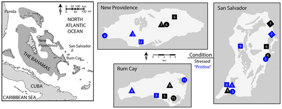
Figure 1.
Map of islands sampled within the Bahamian archipelago (left) and lakes sampled for living and dead ostracod assemblages on each island, with lakes coded for a likely degree of human stress (right). On each island, three to four “stressed lakes” (black icons), subject to historical or current human activities, were paired with physically similar “pristine” lakes (blue icons); icon shapes indicate pairings within each island. Numbers inside icons represent lake-wide species richness, combining living specimens and death assemblages. Adapted with permission from Michelso et al. [47], 2018, Paleobiology.
2.1.2. Wisconsin, USA
Five lakes in the US state of Wisconsin were sampled for living communities and death assemblages of ostracods (Figure 2). Three lakes in the Madison, WI area (lakes Mendota, Monona, and Wingra) were classified as impacted due to a combination of nutrient pollution and the high population density of Madison and its surrounding suburbs. The water quality in all three lakes is regularly monitored by Public Health Madison and Dane Counties, and the annual water quality reports are compiled by the non-profit Clean Lakes Alliance (for example, [59]). The water quality in these lakes has been improving in recent years, yet we classify these lakes as impacted in comparison to two lakes in central Wisconsin (Shadow Lake in Waupaca County and Bullhead Lake in Manitowoc County), where community associations have worked to improve the water quality through a combination of chemical treatments and nutrient mitigation strategies. Shadow and Bullhead Lakes suffered from nutrient pollution and subsequent eutrophication in the mid-twentieth century, similar in degree to the nutrient pollution experienced by the Madison-area lakes. However, unlike the Madison-area lakes, Shadow and Bullhead Lakes were treated with alum (aluminum sulfate) in the 1970s to remove dissolved nutrients from the lake, resulting in precipitation on the lake floor. Subsequently, the local communities have implemented nutrient mitigation efforts (riparian buffers, restrictions on lawn fertilizer, restoration of fish habitat) to maintain the desired mesotrophic to oligotrophic conditions in Shadow and Bullhead Lakes. Thus, we classify Shadow and Bullhead Lakes as remediated in comparison to the Madison-area lakes.
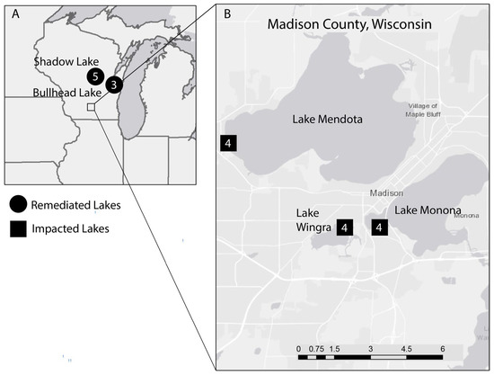
Figure 2.
Map of sampling localities in Wisconsin, USA. (A) shows the localities of the five lakes within the state of Wisconsin, USA. Remediated lakes are designated with a circle and occur in the suburban Waupaca and Manitowoc counties, in central Wisconsin. The urban area of Madison, in southern Wisconsin, is designated by a square in (A), and is shown in more detail in map (B). Map (B) shows the sampling localities for the three urban lakes in Madison County: Lakes Mendota, Monona, and Wingra. Numbers inside icons represent lake-wide species richness, combining living specimens and death assemblages.
2.1.3. Southern California, USA
Bivalves were collected from the Palos Verdes shelf, off the southern coast of the Palos Verdes Peninsula, Los Angeles County, California, USA (Figure 3). White’s Point outfall, one of two major wastewater outfalls serving Los Angeles County and one of six major wastewater outfalls serving southern California, is located on the Palos Verdes Peninsula, as is the Port of Los Angeles. The White’s Point outfall began discharging primary-treated wastewater into the California Bight in 1937, with the discharge reaching a maximum in 1970 [60,61,62]. During the 1950s–1970s, diffusers and intermittent chlorination of the wastewater were used to reduce bacterial contamination of the shoreline waters around Whites Point [62]. Prior to the 1972 Clean Water Act (CWA), the Whites Point outfall also discharged approximately 270 kg/d of DDT-contaminated sewage from Montrose Chemical Corporation [62]. Secondary wastewater treatment was implemented in 1983; by 2002, 100% of the wastewater discharged from White’s Point received secondary treatment [60]. Since the CWA, the water quality in the Southern California Bight has improved dramatically, with suspended solids decreasing by approximately 70% and other pollutants, including heavy metals, decreasing by over 80% [63]. Biological monitoring programs of benthic invertebrates, carried out by the Los Angeles County Sanitation District, also indicate overall improvements to community health since the early 1970s [60]. Based on this environmental history, we are classifying this system as remediated.
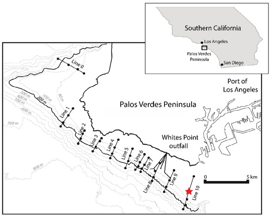
Figure 3.
The Palos Verdes Peninsula is located in Los Angeles County along the Southern California coastline. Lines 1 to 10 are transects used by the Los Angeles County Sanitation District (LACSD) for annual biomonitoring of living macrobenthos. Dots on these lines denote sampling locations at 30, 61, 153, and 305 m. Other lines denote the outfall pipes for the Whites Point outfall. Live assemblages used for this study were collected from 30 m and 61 m along transect Line 10. The red star indicates the location at 50 m where the death assemblages were collected through box coring. Adapted with permission from Leonard-Pingel et al [46], 2019, Marine Ecology Progress Series.
2.2. Sampling Methods
2.2.1. Ostracods
Living communities and associated time-averaged death assemblages were collected from the Bahamian lakes during field expeditions in March 2009 and December 2013. The results from these Bahamian lakes were previously published in Michelson et al. [47]. Comparable living communities and death assemblages were sampled from lakes in the state of Wisconsin, USA, in April 2015 and June 2016, the results of which are reported here for the first time. In both The Bahamas and Wisconsin, eight samples of sediment were collected from each lake sampled. At each point sample, approximately 125 mL of sediment was extracted from the upper 2 cm of sediment. Each sample contains both the remains of dead ostracods in the form of mineralized calcite shells and living benthic individuals that co-occur with the time-averaged remains. To identify the organisms collected alive (or recently dead), Rose Bengal was added to all sediment samples. Rose Bengal stains the chitinous hinge that joins the two valves of the ostracod carapace bright pink [64]. In order to avoid false positives, only those ostracod valves with organic appendages visible (“soft parts”) and stained pink were counted as alive at the time of sampling. Because Rose Bengal will also stain partially decayed organic material, some valves recorded as live individuals may have come from recently deceased organisms (on the scale of weeks to months) but not from the death assemblages representing the last few decades of accumulation.
The sediment samples were stored in plastic containers before the lab analysis. All sediment samples were subdivided into “coarse” (>125 μm) and “fine” (63–125 μm) fractions by wet sieving. The coarse fraction was picked for the ostracod valves using a dissecting microscope. Because of convergent juvenile morphology and multiple molts per individual (between eight and nine), only the valves from adult ostracods were recorded. All valves were identified to species, when possible, following the higher taxonomic classifications of Brandão et al. [65].
2.2.2. Bivalves
Living community data for the bivalves from Southern California were supplied by the Los Angeles Country Sanitation District (LACSD). The LACSD performs annual surveys of the living communities each summer along several transects off the Palos Verdes Peninsula as part of a biomonitoring program (Figure 3). Samples of living individuals were collected using a Van Veen grab (0.1 m2, with 10–15 cm penetration; 1–1.5 L sediment volume per grab), washed on a 1 mm sieve, and picked, counted, and identified to the species level using a standardized regional taxonomy (SCAMIT [66]). The living bivalve assemblage used in this case study is a pooled sample of live bivalves collected in 2009 from the 30 m and 61 m stations of LACSD’s Line 10 (Figure 3). This was completed to approximate the living assemblages at an intermediate depth (50 m) where the death assemblages were collected.
The bivalve death assemblages were collected using a box corer (50 cm × 50 cm) along LACSD’s sampling transect Line 10 at a 50 m depth in September 2012 from the R/V Melville (cruise MV1211). Sampling was conducted as part of a set scientific mission, which is why the collection occurred at 50 m instead of 30 m and 61 m, following the sampling protocol of LACSD. Line 10 is upstream of the Whites Point outfall and, therefore, falls outside the area with the highest effluent deposition, wastewater pollution, and anoxia, but still lies within the range of nutrient-rich waters [61].
The two box cores recovered at this station (PVL10–50m), each penetrating 24 cm into the sediment, were subsampled using smaller plexiglass cores (a 15 cm × 15 cm square cross section) to allow for description and extrusion of the sediment (Figure 4). The subsampling of the box core also allowed us to selectively subsample from the areas of the box core that showed minimal sediment disturbance. The first box core yielded 3 subcores, while the second yielded 4 subcores; the volume of sediment across all subcores in a 2 cm increment was approximately 3 L. After the sediment was extruded from the subcores, it was washed on a 1 mm sieve, the living specimens were removed, and the sieve residue (primarily calcareous shells) was retained for analysis. Dead bivalve shells that retained at least half of the hinge line, or the umbo, were counted as a single individual and identified to the lowest taxonomic unit possible (usually species) using the same standardized regional taxonomy as LACSD (SCAMIT [66]). To make this data consistent with the ostracod data for the case study presented here, we used only the dead bivalve shells collected from the upper 2 cm of the sediment cores. The geochronology of the cores, as well as the presence of burrows visible in the cores, indicates that the cores are probably well-mixed [46]; therefore, the bivalve death assemblages in the upper 2 cm of the core contain a time-averaged assemblage (e.g., shells in this 2 cm increment lived and died at different times) but are likely dominated by shells less than 50 years old [51]. Data from the LACSD living surveys, as well as the complete bivalve death assemblages, have previously been published [46], where additional information about the collection methods and analysis of the bivalve death assemblages for the entire core can be found.
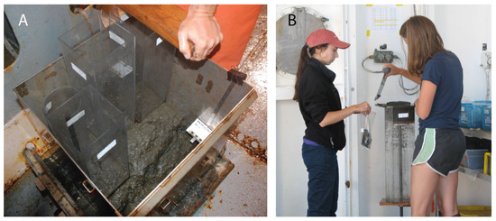
Figure 4.
Sediment sampling onboard the R/V Melville in September 2012: (A) subsampling of a box core; (B) extrusion of 2 cm of sediment from a single plexiglass subcore.
2.3. Data Analysis
Agreement between the living community and associated time-averaged death assemblage in this paper is expressed in all cases using two metrics: Spearman’s rho and the Jaccard-Chao agreement [67], following Kidwell [39,49,68]. Spearman’s rho (hereafter referred to simply as rho) measures the rank-abundance agreement (the absolute abundances of species are converted to ranks) between dead-occurring species and live-occurring species; therefore, it is a measure of agreement in population structure. A maximum value of +1 indicates that the most abundant species in the living assemblage is also the most abundant species in the death assemblage and the least abundant species in the living assemblage is also the least abundant dead species in the death assemblage. A minimum value of −1 indicates a mismatch—the most abundant species in the living assemblage is the least abundant in the death assemblages and vice versa. Jaccard-Chao measures the proportion of shared species between the living communities and death assemblages and thus ranges from 0 to +1. It is a modified version of the Jaccard measure of agreement that is corrected for the “unseen shared species” owing to an under-sampling of the living community, death assemblage, or both [66]. It thus measures the match in species composition between the living communities and death assemblages. These two metrics have become standard practice in conservation paleobiological studies when testing for the live/dead mismatches associated with human impact, e.g., [69,70,71].
For the ostracod live/dead comparisons, agreement metrics were calculated in two ways: with a point-sample scale and a lake (habitat) scale. The point samples reflect living communities and death assemblages at a single location of sampling within a lake. All the lakes sampled are relatively small; therefore, little spatial variation in ecologically meaningful factors exist in these lakes other than the distance from shore [72]. To assess the live/dead agreement at the lake scale, all individuals of the same species from all point samples within a lake were summed together, keeping the live and dead individuals separate. In this way, an estimate of the habitat-scale live/dead agreement was generated by pooling the point samples. The bivalve samples from the Southern California continental shelf are represented by one single point sample; therefore, the point sample is equivalent to the habitat scale.
T-tests were used to test whether differences exist in the means of both the metrics of live/dead agreement in the lakes experiencing different human impacts in the same region: between impacted and “pristine” lakes in the Bahamas and between impacted and remediated lakes in Wisconsin.
3. Results
On the point scale, the live/dead agreement is significantly lower in the impacted lakes than in “pristine” lakes (Bahamas; Figure 5A and Figure 6A,C) and remediated lakes (Wisconsin; Figure 5B and Figure 6B,D) for both metrics of live/dead correspondence. This lower live/dead agreement persists when all point samples from the same environment are pooled to produce one estimate per habitat but lose quantitative significance (The Bahamas, Figure 5C and Figure 6B,D; Wisconsin, Figure 5D and Figure 6B,D). Our sample from Southern California displays a high agreement in species composition but not in population rank abundance (Figure 5B and Figure 6A,C).
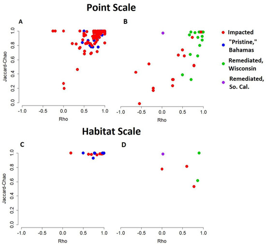
Figure 5.
Live/dead agreement at point (A,B) and habitat scales (C,D) in Bahamian (A,C), as well as Wisconsin and Southern California (B,D) environments. Agreement in population rank abundance is plotted on the x-axis. A value of +1 indicates that the most abundant species in the living community is also the most abundant species in the death assemblage, while a value of −1 indicates that the most abundant species in the living community is the least abundant in the death assemblage. Agreement in species composition is plotted on the y-axis as the proportion (corrected for under-sampling [26]) of species common to both the living community and the death assemblage.
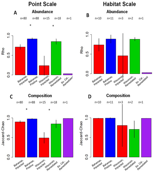
Figure 6.
Bar plots of population rank-abundance agreement, as measured by Spearman’s rho correlation coefficient (A,B) and species composition agreement, as measured by Jaccard-Chao (C,D). Both represent mean live/dead agreement on point- (A,C) and pooled-habitat scales (B,D). Colors correspond to human impact: red represents impacted environments in The Bahamas as well as Wisconsin, while blue represents “pristine” environments in The Bahamas and green-remediated environments in Wisconsin. Southern California is in purple. Error bars represent 95% confidence intervals. Southern California is represented by one sample and therefore lacks error bars. The sample size of each category is listed above each bar plot. An asterisk indicates a significant difference in mean (p < 0.001) live/dead agreement of samples from the same location. Mean live/dead agreement on habitat scale is not significantly different (α = 0.05) in either metric in The Bahamas or Wisconsin.
While the samples from the impacted lakes show significantly lower mean live/dead agreement in population rank-abundance and species composition, they are not uniform. The samples from the impacted lakes show greater variation in both the metrics of live/dead agreement, as some point-scale samples show a high live/dead agreement, such as the unimpacted and remediated lakes (Figure 5A,B and Figure 6A,C).
On the habitat scale, impacted lakes have lower live/dead agreement in both metrics (The Bahamas, Figure 5C; Wisconsin, Figure 5D); however, this reduced live/dead agreement is not statistically significant (α = 0.05) in either metric of agreement (population rank abundance, Figure 6B; species composition, Figure 6D). Southern California is represented by one sample; therefore, the habitat scale is equivalent to the point scale.
4. Discussion
4.1. Live–Dead Discordance in Impacted Ecosystems
A mismatch between the living and the death assemblage occurs as species are gained or lost from a community and as the relative abundances of species change in that community in response to anthropogenic impacts. Because of this, the individuals found in the death assemblages but not in the living assemblages could indicate local extirpations, e.g., [48]. These “canaries” [47] can be used as indicators of environmental and ecological deterioration over historical or modern time. In addition, changes in the relative abundances of species (indicated by rho), can indicate changes in community structure due to human impact on the system.
Throughout the analysis presented above, we see many instances of the ecosystems classified as impacted falling into the low fidelity or very low fidelity quadrants defined by Kidwell [39,67], indicating that human activities have caused an ecological response within the time span over which death assemblages have accumulated (Figure 5 and Figure 6). This discordance appears to be particularly visible on the point scale for both impacted lakes of The Bahamas and Wisconsin. The higher instances of discordance on the point scale may be due to a higher variability inherent to single samples/small sample sizes. For example, a living individual of a particular species may be easily missed at a single point but may be retrieved when all samples in a lake are examined and pooled. Regardless of this higher variability or the potential impact of smaller sampling sizes, it is important to note that none of the point scale samples from the “pristine” environments fall into the low or very low fidelity quadrants (Figure 5A), indicating that a high fidelity of living and death assemblages can be expected, even on the point scale, in the low-impact, “pristine” ecosystems.
Some of the lakes with the highest discordance from The Bahamas are lakes that have a history of impact during the plantation era (late eighteenth to mid-nineteenth centuries) but that are relatively removed from human settlements or experienced a relatively low impact in the modern era (the Watlings Blue Hole and Salt Pond). This high discordance in the live–dead comparisons is somewhat unexpected, as it might be anticipated that recovery of the ecosystem should have taken place by this time. The disparity is due to the loss of four species in the living assemblages (e.g., four species that are found only in the death assemblages) in these two lakes. Because these four species are found living in other nearby lakes that are considered “pristine,” the interpretation is that these species were lost during the colonial period, at the time of highest human impact, and indicate a legacy condition/prolonged recovery of the ecosystem [47]. This example, coupled with other examples from marine systems (e.g., [48]), demonstrates the utility of live–dead discordance in discovering human-induced taxonomic loss and recalcitrant ecosystem recovery.
It is possible that a live–dead survey in an impacted environment may fall in the high-fidelity quadrant, particularly when looking at the habitat scale (Figure 5C,D). This does not mean that the community is not at risk. A high fidelity of live–dead assemblages in impacted environments could indicate that the impact has not been prolonged or acute enough to cause ecological turnover. On the other hand, agreement between living and dead communities in impacted settings could also occur when the impact has been so long-standing that the death assemblage reflects that human impact [38]; this may be the case for some of the lakes in Wisconsin, where human impact stretches back to the mid-eighteen hundreds, or in some of the lakes in The Bahamas that experienced plantation-era impacts but show a high fidelity in live/dead assemblages. In cases where this is suspected, it may be wise to explore the possibility of collecting short sediment cores to provide a longer time scale for comparison, e.g., [46].
The degree of discordance between living and death assemblages may depend on the scale at which samples are being compared (Figure 5 and Figure 6). Impacted lakes from The Bahamas and Wisconsin both show variability among the point scale live–dead discordance comparisons from samples within the same lake. This variability may be higher when habitats are large, have high variability with regard to environmental parameters (e.g., substrate type, water depth), or have a variable level of impact (e.g., high-density development on one side of a lake compared to the other). To combat this, we recommend that the discordance be analyzed on both a point scale as well as a habitat scale.
4.2. Live–Dead Discordance in Remediated Ecosystems
In the same way that the degree of fidelity between living and death assemblages can be used to identify human impact, it can also be used to determine if conservation or management efforts to restore a previously impacted system are effective. In these case studies, we show that several live/dead collections from remediated ecosystems fall in the “high fidelity” quadrant. In the case studies from the Wisconsin lakes and the southern California coastline, both examples of areas that experienced remediation for eutrophication beginning in the 1970s, live/dead comparisons showing high fidelity could indicate the success of the remediation attempts (e.g., a return to a pre-impact community preserved in the death assemblage, as suggested in [46]).
The Southern California case study shows good agreement in the species’ compositions between the living communities and death assemblages (a high Jaccard-Chao value) but a relatively low agreement in the population structure/rank order abundance (a lower rho value). In this case, the death assemblage contains a high proportion of the pollution-tolerant and nutrient-loving bivalve, Parvilucina, which was abundant during the 1970s at the height of eutrophication but has since declined in abundance due to wastewater treatment (e.g., remediation) [46]. In this case, the death assemblage records a historic nineteenth-century human impact, while the living assemblage shows a return to a more “natural” population structure, which is observed in the lower rho value. In this case, system recovery is only completely understood when the changes in the death assemblages in the entire core are considered [46], illustrating the need to consider the time scale of impact when using the death assemblages as a measure of recovery. As discussed above, when human impacts are long-standing and acute (as in the case in Southern California), there may be very little mismatch in the live–dead comparisons. In these cases, longer records will be necessary to create baselines for natural communities.
Remediated lakes from Wisconsin (Shadow Lake and Bullhead Lake) also show a high fidelity between the living and death assemblages, with all the habitat scale comparisons and nearly all point-scale comparisons falling into the highest fidelity quadrant (Figure 5). We interpret this as an indication that local community-level efforts to remediate the lakes (e.g., riparian buffers, restoration of fish habitats) have been effective in reducing eutrophication and ecosystem disruption. This is in stark comparison with the impacted urban lakes in Wisconsin that have not been remediated, and which show much lower overall live–dead fidelity (Figure 5B,D) and have both significantly lower rho and Jaccard-Chao values on the point scale (Figure 6A,C). The impact length and sedimentation rates are estimated to be approximately the same in all these lakes; therefore, we attribute the differences in discordance to be primarily due to remediation. Successful remediation of Shadow Lake is confirmed by core-based studies of ostracods and diatoms. Thus, these case studies indicate that a comparison of live–dead communities could also be an effective tool in assessing the remediation attempts.
4.3. Time–Averaging in Death Assemblages
The time scale that is captured in the death assemblage can vary among habitats, depending on the degree of time-averaging of the skeletal components. In continental shelf environments, such as that of our Southern California case study, bivalve assemblages can contain individual valves that are several millennia old in the upper 8 cm of the sediment column [51,52,53,54]; this may also be the case for the molluskan assemblages in some lakes [73]. Based on radioisotopic dating of the sediments in which they occur, we suspect that the time-averaging of the ostracod assemblages presented in these case studies is multi-decadal. Future work using direct dating of the ostracod shells will allow for more precise estimates of the window of time-averaging of these death assemblages.
In cases where time-averaging is suspected to be on the order of centuries to millennia, as in our Southern California case study, the death assemblage will contain individuals that span a wide gradient of human impact. On the other hand, death assemblages from lakes or other habitats with high sedimentation rates may experience much less time-averaging. In these cases, the death assemblages may only contain individuals from the past few decades. Differences in production rates (biologically driven) and sedimentation rates (environmentally driven) will impact the amount of time-averaging in a system. This variability should be understood as much as possible in a system and accounted for when making interpretations about community changes and their responses to human impact.
5. Conclusions
The case studies presented here demonstrate the effectiveness of live/dead comparisons in identifying ecosystems that have been affected by human impacts. A single survey of the living assemblage compared to the death assemblage has the potential to demonstrate a change in community composition and/or structure, thereby indicating a human modification of the natural ecosystem. A comparison of live–dead assemblages, or the reconstruction of a historic ecosystem change using short cores, can also indicate local extirpations, legacy impacts, and can be used as a measure of ecosystem recovery in remediated or managed systems. The collection of death assemblages is low-tech low-cost, especially in terrestrial freshwater environments, making it accessible to a variety of scientists, managers, and organizations globally. The processing of death assemblages and the identification and quantification of taxa preserved in death assemblages can be time-consuming; however, the time cost could be minimized in cases where there are bio-indicators or key species of interest that could be targeted. Live–dead surveys in targeted areas (e.g., currently managed systems, systems targeted for remediation) also present an opportunity to expand citizen science efforts or community-engaged research [74].
Death assemblages can provide long-term data (multi-decadal in most cases) that can prove key in the establishment of conservation baselines and can provide context to biodiversity changes to help bring to light the invisible biodiversity loss occurring in many invertebrate groups. Therefore, we strongly urge the use of death assemblages to supplement ongoing biodiversity surveys and biomonitoring data, especially where invertebrates with mineralized skeletal remains play an important role in the ecosystem.
Author Contributions
J.S.L.-P. and A.V.M. contributed to writing the manuscript; J.S.L.-P. and A.V.M. performed fieldwork and data collection; J.S.L.-P. contributed the bivalve data from Southern California; A.V.M. and L.P.B. contributed the ostracod data from The Bahamas, while A.V.M. contributed the ostracod data from Wisconsin; A.V.M. performed statistical analyses; J.J.S., K.C.K. and L.P.B. contributed to the study’s design and ostracod data collection. All authors have read and agreed to the published version of the manuscript.
Funding
The collection of Bahamian samples was enabled by the National Science Foundation (US) grants EAR-1249831 to AVM and EAR-0851847 to LPB. The collection of samples from Southern California was enabled by NSF EAR 1124189, awarded to S. Kidwell and A. Tomašových. The collection of Wisconsin samples was enabled by sub-award from the Keck Geology Consortium, NSF awarded to J.L.-P. and AVM, funded by NSF REU-1358987.
Institutional Review Board Statement
Not applicable.
Data Availability Statement
A complete dataset for the Southern California bivalves is available in the supplementary material for Leonard-Pingel et al 2019 [46]. The complete dataset for ostracods from The Bahamas is available in the Dryad Digital Repository: https://datadryad.org/stash/dataset/doi:10.5061/dryad.8sp77v5, (accessed on 26 May 2023).
Acknowledgments
The collection of Bahamian samples was carried out under permits G252, G234, and G235 from the Bahamas Environment, Science and Technology Commission. Living surveys from LACSD were made available by D. Cadien. S. Kidwell provided helpful, thoughtful, and constructive advice on the use and interpretation of live/dead agreement. We are grateful to J. Ash, V. Haley-Benjamin, L. Knowles, S. Bright, M. Dalman, E. Frank, E. Draher, S. Bua-Iam, A. Conaway, J. Dannehl, S. Garelick, T. Mooney, and A. Waheed for their invaluable field assistance. K. Brady Shannon, A. Myrbo, and the Continental Scientific Drilling Facility (formerly National Lacustrine Core Facility) provided indispensable logistical and scientific support. E. and T. Rothfus of the Gerace Research Centre enabled the collection of Bahamian samples by managing communications with the Bahamian government. M. Davila-Banrey, O. Diana, S. Fitzpatrick, and M. Viteri provided valuable lab assistance.
Conflicts of Interest
The authors declare no conflict of interest.
References
- Barnosky, A.D.; Matzke, N.; Tomiya, S.; Wogan, G.O.U.; Swartz, B.; Quental, T.B.; Marshall, C.; McGuire, J.L.; Lindsey, E.L.; Maguire, K.C.; et al. Has the Earth’s sixth mass extinction already arrived? Nature 2011, 471, 51–57. [Google Scholar] [CrossRef] [PubMed]
- Ceballos, G.; Ehrlich, P.R.; Dirzo, R. Biological annihilation via the ongoing sixth mass extinction signaled by vertebrate population losses and declines. Proc. Natl. Acad. Sci. USA 2017, 114, E6089–E6096. [Google Scholar] [CrossRef] [PubMed]
- Tilman, D.; May, R.; Lehman, C.; Nowak, M.A. Habitat destruction and the extinction debt. Nature 1994, 371, 65–66. [Google Scholar] [CrossRef]
- Kuussaari, M.; Bommarco, R.; Heikkinen, R.K.; Helm, A.; Krauss, J.; Lindborg, R.; Öckinger, E.; Pärtel, M.; Pino, J.; Rodà, F.; et al. Extinction debt: A challenge for biodiversity conservation. Trends Ecol. Evol. 2009, 24, 564–571. [Google Scholar] [CrossRef]
- Halley, J.M.; Monokrousos, N.; Mazaris, A.D.; Newmark, W.D.; Vokou, D. Dynamics of extinction debt across five taxonomic groups. Nat. Commun. 2016, 7, 12283. [Google Scholar] [CrossRef]
- Spalding, C.; Hull, P.M. Towards quantifying the mass extinction debt of the Anthropocene. Proc. R. Soc. B 2021, 288, 20202332. [Google Scholar] [CrossRef]
- Ceballos, G.; Ehrlich, P.R.; Raven, P.H. Vertebrates on the brink as indicators of biological annihilation and the sixth mass extinction. Proc. Natl. Acad. Sci. USA 2020, 117, 13596–13602. [Google Scholar] [CrossRef]
- Ceballos, G.; Ehrlich, P.R.; Barnosky, A.D.; García, A.; Pringle, R.M.; Palmer, T.M. Accelerated modern human-induced species losses: Entering the sixth mass extinction. Sci. Adv. 2015, 1, e1400253. [Google Scholar] [CrossRef]
- Dirzo, R.; Young, H.S.; Galetti, M.; Ceballos, G.; Isaac, N.J.B.; Collen, B. Defaunation in the Anthropocene. Science 2014, 345, 401–406. [Google Scholar] [CrossRef]
- Erwin, D.H. Extinction: How Life on Earth Nearly Ended 250 Million Years Ago; Princeton University Press: Princeton, NJ, USA, 2006. [Google Scholar]
- Cardinale, B. Impacts of biodiversity loss. Science 2012, 336, 552–553. [Google Scholar] [CrossRef] [PubMed]
- Naeem, S.; Duffy, J.E.; Zavaleta, E. The Functions of Biological Diversity in an Age of Extinction. Science 2012, 336, 1401–1406. [Google Scholar] [CrossRef] [PubMed]
- Estes, J.A.; Terborgh, J.; Brashares, J.S.; Power, M.E.; Berger, J.; Bond, W.J.; Carpenter, S.R.; Essington, T.E.; Holt, R.D.; Jackson, J.B.C.; et al. Trophic Downgrading of Planet Earth. Science 2011, 333, 301–306. [Google Scholar] [CrossRef]
- Vörösmarty, C.J.; McIntyre, P.B.; Gessner, M.O.; Dudgeon, D.; Prusevich, A.; Green, P.; Glidden, S.; Bunn, S.E.; Sullivan, C.A.; Reidy Lierman, C.; et al. Global threats to human water security and river biodiversity. Nature 2010, 467, 555–561. [Google Scholar] [CrossRef] [PubMed]
- Collen, B.; Böhm, M.; Kemp, R.; Baillie, J.E.M. Spineless: Status and Trends of the World’s Invertebrates; Zoological Society: London, UK, 2012; p. 88. [Google Scholar]
- Macadam, C.R.; Stockan, J.A. More than just fish food: Ecosystem services provided by freshwater insects. Ecol. Entomol. 2015, 40, 113–123. [Google Scholar] [CrossRef]
- Potts, S.G.; Imperatriz-Fonseca, V.; Ngo, H.T.; Aizen, M.A.; Biesmeijer, J.C.; Breeze, T.D.; Dicks, L.V.; Garibaldi, L.A.; Hill, R.; Settele, J.; et al. Safeguarding pollinators and their values to human well-being. Nature 2016, 540, 220–229. [Google Scholar] [CrossRef] [PubMed]
- Soliveres, S.; Van Der Plas, F.; Manning, P.; Prati, D.; Gossner, M.M.; Renner, S.C.; Alt, F.; Arndt, H.; Baumgartner, V.; Binkenstein, J.; et al. Biodiversity at multiple trophic levels is needed for ecosystem multifunctionality. Nature 2016, 536, 456–459. [Google Scholar] [CrossRef]
- Greenop, A.; Woodcock, B.A.; Outhwaite, C.L.; Carvell, C.; Pywell, R.F.; Mancini, F.; Edwards, F.K.; Johnson, A.C.; Isaac, N.J. Patterns of invertebrate functional diversity highlight the vulnerability of ecosystem services over a 45-year period. Curr. Biol. 2021, 31, 4627–4634. [Google Scholar] [CrossRef]
- Schipper, J.; Chanson, J.S.; Chiozza, F.; Cox, N.A.; Hoffmann, M.; Katariya, V.; Lamoreux, J.; Rodrigues, A.S.; Stuart, S.N.; Temple, H.J.; et al. The status of the world’s land and marine mammals: Diversity, threat, and knowledge. Science 2008, 322, 225–230. [Google Scholar] [CrossRef]
- Régnier, C.; Bouchet, P.; Hayes, K.A.; Yeung, N.W.; Christensen, C.C.; Chung, D.J.D.; Fontaine, B.; Cowie, R.H. Extinction in a hyperdiverse endemic Hawaiian land snail family and implications for the underestimation of invertebrate extinction. Conserv. Biol. 2015, 29, 1715–1723. [Google Scholar] [CrossRef]
- Ricciardi, A.; Rasmussen, J.B. Extinction rates of North American freshwater fauna. Conserv. Biol. 1999, 13, 1220–1222. [Google Scholar] [CrossRef]
- McKinney, M.L. High rates of extinction and threat in poorly studied taxa. Conserv. Biol. 1999, 13, 1273–1281. [Google Scholar] [CrossRef]
- Hallman, C.A.; Sorg, M.; Jongejans, E.; Siepel, H.; Hofland, N.; Schwan, H.; Stenmans, W.; Müller, A.; Sumser, H.; Hörren, T.; et al. More than 75 percent decline over 27 years in total flying insect biomass in protected areas. PLoS ONE 2017, 12, e0185809. [Google Scholar] [CrossRef]
- Thomas, J.A.; Telfer, M.G.; Roy, D.B.; Preston, C.D.; Greenwood, J.J.D.; Asher, J.; Fox, R.; Clarke, R.T.; Lawton, J.H. Comparative losses of British butterflies, birds, and plants and the global extinction crisis. Science 2004, 303, 1879–1881. [Google Scholar] [CrossRef] [PubMed]
- Dudgeon, D.; Arthington, A.H.; Gessner, M.O.; Kawabata, Z.I.; Knowler, D.J.; Lévêque, C.; Naiman, R.J.; Prieur-Richard, A.H.; Soto, D.; Stiassny, M.L.; et al. Freshwater biodiversity: Importance, threats, status and conservation challenges. Biol. Rev. 2006, 81, 163–182. [Google Scholar] [CrossRef]
- Wilson, E.O. The little things that run the world (the importance and conservation of invertebrates). Conserv. Biol. 1987, 1, 344–346. [Google Scholar] [CrossRef]
- Stuart, S.N.; Wilson, E.O.; McNeely, J.A.; Mittermeier, R.A.; Rodríguez, J.P. Response: Barometer of Life. Science 2010, 329, 141–142. [Google Scholar] [CrossRef]
- Régnier, C.; Fontaine, B.; Bouchet, P. Not knowing, not recording, not listing: Numerous unnoticed mollusk extinctions. Conserv. Biol. 2009, 23, 1214–1221. [Google Scholar] [CrossRef]
- Eisenhauer, N.; Bonn, A.A.; Guerra, C. Recognizing the quiet extinction of invertebrates. Nat. Commun. 2019, 10, 50. [Google Scholar] [CrossRef] [PubMed]
- Gerlach, J.; Samways, M.J.; Hochkirch, A.; Seddon, M.; Cardoso, P.; Clausnitzer, V.; Cumberlidge, N.; Daniel, B.A.; Black, S.H.; Ott, J.; et al. Prioritizing non-marine invertebrate taxa for Red Listing. J. Insect Conserv. 2014, 18, 573–586. [Google Scholar] [CrossRef]
- McClenachan, L. Historical declines of goliath grouper populations in South Florida, USA. Endang. Species Res. 2009, 7, 175–181. [Google Scholar] [CrossRef]
- McClenachan, L.; Cooper, A.B. Extinction rate, historical population structure and ecological role of the Caribbean monk seal. Proc. Biol. Sci. 2008, 275, 1351–1358. [Google Scholar] [CrossRef]
- McClenachan, L.; Jackson, J.B.C.; Newman, M.J.H. Conservation implications of historic sea turtle nesting beach loss. Front. Ecol. Environ. 2006, 4, 290–296. [Google Scholar] [CrossRef]
- Rosenberg, A.A.; Bolster, W.J.; Alexander, K.E.; Leavenworth, W.B.; Cooper, A.B.; McKenzie, M.G. The history of ocean resources: Modeling cod biomass using historical records. Front. Ecol. Environ. 2005, 3, 78–84. [Google Scholar] [CrossRef]
- McClenachan, L.; Ferretti, F.; Baum, J.K. From archives to conservation: Why historical data are needed to set baselines for marine animals and ecosystems. Conserv. Lett. 2012, 5, 349–359. [Google Scholar] [CrossRef]
- Jackson, J.B.; Kirby, M.X.; Berger, W.H.; Bjorndal, K.A.; Botsford, L.W.; Bourque, B.J.; Bradbury, R.H.; Cooke, R.; Erlandson, J.; Estes, J.A.; et al. Historical overfishing and the recent collapse of coastal ecosystems. Science 2001, 293, 629–637. [Google Scholar] [CrossRef]
- Kidwell, S.M.; Tomašových, A. Implications of Time-Averaged Death Assemblages for Ecology and Conservation Biology. Annu. Rev. Ecol. Evol. Syst. 2013, 44, 539–563. [Google Scholar] [CrossRef]
- Kidwell, S.M. Time-averaging and the fidelity of modern death assemblages: Building a taphonomic framework for conservation paleobiology. Palaeontology 2013, 56, 487–522. [Google Scholar] [CrossRef]
- Best, M.M.; Kidwell, S.M. Bivalve taphonomy in tropical mixed siliciclastic-carbonate settings. I. Environmental variation in shell condition. Paleobiology 2000, 26, 80–102. [Google Scholar] [CrossRef]
- Behrensmeyer, A.K.; Kidwell, S.M.; Gastaldo, R.A. Taphonomy and paleobiology. Paleobiology 2000, 26 (Suppl. S4), 103–147. [Google Scholar] [CrossRef]
- Flessa, K.W.; Cutler, A.H.; Meldahl, K.H. Time and taphonomy: Quantitative estimates of time-averaging and stratigraphic disorder in a shallow marine habitat. Paleobiology 1993, 19, 266–286. [Google Scholar] [CrossRef]
- Kidwell, S.M.; Bosence, D.W.J. Taphonomy and Time-averaging of Marine Shelly Faunas. In Taphonomy: Releasing the Data Locked in the Fossil Record; Kidwell, S.M., Bosence, D.W., Allison, P.A., Briggs, D.E.G., Eds.; Plenum: New York, NY, USA, 1991; pp. 115–209. [Google Scholar]
- Behrensmeyer, A.K. Taphonomic and ecologic information from bone weathering. Paleobiology 1978, 4, 150–162. [Google Scholar] [CrossRef]
- Meadows, C.A.; Grebmeier, J.M.; Kidwell, S.M. High-latitude benthic bivalve biomass and recent climate change: Testing the power of live-dead discordance in the Pacific Arctic. Deep-Sea Res. II 2019, 162, 152–163. [Google Scholar] [CrossRef]
- Leonard-Pingel, J.S.; Kidwell, S.M.; Tomašových, A.; Alexander, C.R.; Cadien, D.B. Gauging benthic recovery from 20th century pollution on the southern California continental shelf using bivalves from sediment cores. Mar. Ecol. Prog. Ser. 2019, 615, 101–119. [Google Scholar] [CrossRef]
- Michelson, A.V.; Kidwell, S.M.; Park Boush, L.E.; Ash, J.E. Testing for human impacts in the mismatch of living and dead ostracode assemblages at nested spatial scales in subtropical lakes from the Bahamian archipelago. Paleobiology 2018, 44, 758–782. [Google Scholar] [CrossRef]
- Tomašových, A.; Kidwell, S.M. Ninteenth-century collapse of a benthic marine ecosystem on the open continental shelf. Proc. R. Soc. B 2017, 284, 20170328. [Google Scholar] [CrossRef]
- Kidwell, S.M. Discordance between living and death assemblages as evidence for anthropogenic ecological change. Proc. Natl. Acad. Sci. USA 2007, 104, 17701–17706. [Google Scholar] [CrossRef]
- Tomašových, A.; Kidwell, S.M.; Alexander, C.R.; Kaufman, D.S. Millennial-scale age offsets within fossil assemblages: Result of bioturbation below the taphonomic active zone and out-of-phase production. Paleoceano. Paleoclim. 2019, 34, 954–977. [Google Scholar] [CrossRef]
- Dominguez, J.G.; Kosnik, M.A.; Allen, A.P.; Hua, Q.; Jacob, D.E.; Kaufman, D.S.; Whitacre, K. Time-averaging and stratigraphic resolution in death assemblages and Holocene deposits: Sydney Harbour’s molluscan record. Palaios 2016, 31, 564–575. [Google Scholar] [CrossRef]
- Krause, R.A.; Barbour, S.L.; Kowalewski, M.; Kaufman, D.S.; Romanek, C.S.; Simoes, M.G.; Wehmiller, J.F. Quantitative comparisons and models of time-averaging in bivalve and brachiopod shell accumulations. Paleobiology 2010, 36, 428–452. [Google Scholar] [CrossRef]
- Kosnik, M.A.; Hua, Q.; Kaufman, D.S.; Wüst, R.A. Taphonomic bias and time-averaging in tropical molluscan death assemblages: Differential shell half-lives in Great Barrier Reef sediment. Paleobiology 2009, 35, 565–586. [Google Scholar] [CrossRef]
- Hull, P.M.; Darroch, S.A.; Erwin, D.H. Rarity in mass extinctions and the future of ecosystems. Nature 2015, 528, 345–351. [Google Scholar] [CrossRef]
- Tomašových, A.; Kidwell, S.M. Fidelity of variation in species composition and diversity partitioning by death assemblages: Time-averaging transfers diversity from beta to alpha levels. Paleobiology 2009, 35, 94–118. [Google Scholar] [CrossRef]
- Tomašových, A.; Kidwell, S.M. Predicting the effects of increasing temporal scale on species composition, diversity, and rank-abundance distributions. Paleobiology 2010, 36, 672–695. [Google Scholar] [CrossRef]
- Tomašových, A.; Kidwell, S.M. Accounting for the effects of biological variability and temporal autocorrelation in assessing the preservation of species abundance. Paleobiology 2011, 37, 332–354. [Google Scholar] [CrossRef]
- Van Leeuwen, J.F.; Froyd, C.A.; van der Knaap, W.O.; Coffey, E.E.; Tye, A.; Willis, K.J. Fossil pollen as a guide to conservation in the Galápagos. Science 2008, 322, 1206. [Google Scholar] [CrossRef]
- Wynn, L. 2021 Water Quality Monitoring Results. Clean Lakes Alliance. Available online: https://www.cleanlakesalliance.org/2021-water-quality-monitoring-results/ (accessed on 30 August 2022).
- Stein, E.D.; Cadien, D. Ecosystem response to regulatory and management actions: The southern California experience in log-term monitoring. Mar. Pollut. Bull. 2009, 59, 91–100. [Google Scholar] [CrossRef]
- Stull, J.K.; Swift, D.J.P.; Niedoroda, A.W. Contaminant dispersal on the Palos Verdes continental margin: I. Sediments and biota near a major California wastewater discharge. Sci. Total Environ. 1996, 179, 73–90. [Google Scholar] [CrossRef]
- Schafer, H. Improving Southern California’s Coastal Waters. J. Water Pollut. Control. Fed. 1989, 61, 1394–1401. [Google Scholar]
- Lyon, G.S.; Stein, E.D. How effective has the Clean Water Act been at reducing pollutant mass emissions to the Southern California Bight over the past 35 years? Environ. Monit. Assess. 2009, 154, 413–426. [Google Scholar] [CrossRef] [PubMed]
- Corrège, T. The relationship between water masses and benthic ostracod assemblages in the western Coral Sea, southwest Pacific. Palaeogeo. Palaeoclim. Palaeoeco. 1993, 105, 245–266. [Google Scholar] [CrossRef]
- Brandão, S.N.; Angel, M.V.; Karanovic, I.; Perrier, V.; Yasuhara, M. 2021. World Ostracoda Database. World Register of Marine Species. Available online: http://www.marinespecies.org/aphia.php?p=taxdetails&id=1078 (accessed on 26 May 2023).
- SCAMIT (Southern California Association of Marine Invertebrate Taxonomists). A Taxonomic Listing of benthic Macro- and Megainvertebrates from Infaunal and Epifaunal Monitoring and Research Programs in the Southern California Bight, 8th ed.; SCAMIT: San Diego, CA, USA, 2013. [Google Scholar]
- Chao, A.; Chazdon, R.L.; Colwell, R.K.; Shen, T.-J. A new statistical approach for assessing compositional similarity based on incidence and abundance data. Ecol. Lett. 2005, 8, 148–159. [Google Scholar] [CrossRef]
- Kidwell, S.M. Biology in the Anthropocene: Challenges and insights from young fossils records. Proc. Natl. Acad. Sci. USA 2015, 112, 4922–4929. [Google Scholar] [CrossRef] [PubMed]
- Casey, M.M.; Dietl, G.P.; Post, D.M.; Briggs, D.E. The impact of eutrophication and commercial fishing on molluscan communities in Long Island Sound, USA. Biol. Cons. 2014, 170, 137–144. [Google Scholar] [CrossRef]
- Smith, J.A.; Dietl, G.P. The value of geohistorical data in identifying a recent human-inducved range expansion of a predatory gastropod in the Colorado River delta, Mexico. J. Biogeogr. 2016, 43, 791–800. [Google Scholar] [CrossRef]
- Smith, J.A.; Dietl, G.P.; Durham, S.R. Increasing the salience of marine live-dead data in the Anthropocene. Paleobiology 2020, 46, 279–287. [Google Scholar] [CrossRef]
- Michelson, A.V.; Park, L.E. Taphonomic dynamics of lacustrine ostracodes on San Salvador Island, Bahamas: High fidelity and evidence of anthropogenic modification. Palaios 2013, 28, 129–135. [Google Scholar] [CrossRef]
- Leonard-Pingel, J.; Bua-Iam, S.; Kaufman, D.S.; Tomašových, A. Extensive time-averaging in lacustrine gastropod assemblages from Shadow Lake, Waupaca, Wisconsin. In Proceedings of the Geological Society of America Annual Meeting, Phoenix, AZ, USA, 22–25 September 2019; Geological Society of America (GSA): Boulder, CO, USA, 2019; Volume 51. No. 5; paper 285-15; Abstracts with Programs 2019. [Google Scholar]
- Leonard-Pingel, J.S.; Michelson, A.V.; Wittmer, J.M.; Bhattacharya, A.; Arora, G.; Ray, R. Closing the science-society gap by engaging community partners in conservation paleobiology field studies. In Proceedings of the Geological Society of America Annual Meeting, Denver, CO, USA, 9–12 October 2022; Geological Society of America (GSA): Boulder, CO, USA, 2022; Volume 54. No. 5 paper 132-4; Abstracts with programs 2022. [Google Scholar]
Disclaimer/Publisher’s Note: The statements, opinions and data contained in all publications are solely those of the individual author(s) and contributor(s) and not of MDPI and/or the editor(s). MDPI and/or the editor(s) disclaim responsibility for any injury to people or property resulting from any ideas, methods, instructions or products referred to in the content. |
© 2023 by the authors. Licensee MDPI, Basel, Switzerland. This article is an open access article distributed under the terms and conditions of the Creative Commons Attribution (CC BY) license (https://creativecommons.org/licenses/by/4.0/).