Article

Assessment of Habitat Selection by Invasive Plants and Conditions with the Best Performance of Invasiveness Traits

by
Emilia Grzędzicka
Institute of Systematics and Evolution of Animals, Polish Academy of Sciences, Sławkowska 17, 31-016 Kraków, Poland
Diversity 2023, 15(3), 333; https://doi.org/10.3390/d15030333
Submission received: 29 December 2022 / Revised: 14 February 2023 / Accepted: 23 February 2023 / Published: 25 February 2023

Abstract

:
Habitat selection is one of the fundamental concepts in ecology and means that each organism should choose the habitat that will maximize its success. Invaders may be an underestimated object in research on habitat selection. Invasive plants experience enormous propagule pressure and bear the costs of spreading in disturbed anthropogenic habitats. It means that they do not necessarily achieve maximum invasiveness traits in such habitats, which they selected to colonize. This study aimed to assess habitats where invaders are likely to occur from the set of all available ones in the landscape and the habitats with the best performed traits of invaders. The research was conducted on 52 and 112 plots in 2019 and 2021, respectively, in South-Eastern Poland, and the invasive plants were Caucasian hogweeds Heracleum sp. In the first year, the circle plots had a 50 m radius and were to measure habitat areas and traits of hogweeds (height, number of individuals in the plot, cover, and number of flowering specimens). Detrimental correspondence analysis and linear mixed model investigated that hogweeds achieved the best performance reflected by traits in continuous habitats—meadows and forests. In the second year, the plots to measure habitats had a 100 m radius. The reference plots were far from the invasion exposure, and the paired control vs. Heracleum ones had the same habitats with the potential to be invaded. The generalized linear mixed model showed that the probability of the hogweeds occurrence was higher when the habitat was overgrowing with a simultaneous decrease in open areas and in the increasing ruderal area with a decrease in bushes. The impact of the invader’s habitat on the invasion performance depended on the purpose of habitat selection. When invaders spread and increased invasive extent or appeared in habitat edges, they did not reach the highest traits, the best performing in continuous habitats. The specificity of habitat selection of invaders is another aspect that distinguishes invasion science from classic ecology.

1. Introduction

The spreading of invasive plants is among the most important environmental and socio-economic problems [1,2,3]. Invasion science is a dynamically developing field, which should provide tools for predicting and preventing the effects of invasions. However, many invasions are unlikely to be stopped, and the landscape with them is more often treated as a research system to verify the rules of ecology [4]. In contrast with classic ecology, organisms facing invasions compete primarily with individuals of their species rather than with other taxa. The reasons are interspecific differences in resource use and spatial relationships between responses of various species to the environment and competition with others [5]. Alien species compete also with native species and under low resource availability, both are similarly competitive [6]. A novel trend is assuming the invasive species as ecosystem engineers causing interactions between habitats and the organisms [7]. Modern habitats with unpredictable changes are highly vulnerable to plant invasions [6]. There is an urgent need for research on invasion ecology, which is a real “crisis science” rather than only another scientific exercise.
One of the most important concepts in classic ecology is habitat selection, according to which each organism should choose conditions that maximize its survival, reproduction, and growth [8,9]. Due to the logarithmic increase in the population of invasive organisms, their success depends on the selected habitat conditions, so they are an ideal research object that can contribute to the knowledge about habitat selection [10]. However, in a disturbed environment or favorable conditions, e.g., in uncrowded populations, native plants can also show exponential population growth [11]. The difference between alien and native species is that aliens exist in an environment from which they do not come, so their habitat selection will always be riskier than in the case of natives. Alien species can be considered as “settlers”, for some reason selecting particular habitats despite the fact they are new to them [12]. If the habitats are all equally exposed to invasions, alien species would occur randomly in the landscape in individual habitats proportionally to their availability. However, habitats have different susceptibilities to invasive species. Assuming that the invader tries to occupy all types of habitats, but succeeds only in some of them, preventing the spread of alien species should concentrate on such invasion-prone habitats [12]. Any action aimed at reducing the effect of invasions requires research on the extent to which different habitats are susceptible to invasions [13,14].
Understanding invasion rapid spread patterns and the underlying processes driving invasions are key to predicting invasion. Any habitat features that influence alien population growth or dispersal can affect the rate of spread [15]. Phenomena favoring habitat invasibility are a disturbance, early successional environment, and low diversity of native species [16]. Disturbances can facilitate invasions due to the associated increase in resource availability [17]. It means that there must be a shortage of resources for native organisms facing disturbance, natives abandon the habitat, and then the invaders, as low-demanding species, immediately use the abandoned resources. This space is located in a specific landscape matrix and thus surrounded by habitats that can again facilitate or inhibit the development of the invasion. Understanding the mechanisms causing such heterogeneity usefulness in the rate of invasion spread is key to predicting future spread and identifying important locations for management [4,15].
As mentioned, the feature linking all habitats exposed to invasions is a disturbance. For example, the most invasible habitat, arable lands, experiences a complete removal of aboveground biomass at least once a year [13]. It means regular disturbances and later restorations during succession, in which the most successful are pioneer, low-demanding organisms [18]. Then, species richness and diversity increase with the succession progress, although organisms intensively compete for resources [19]. Ruderal vegetation (i.e., degraded herbaceous plant communities of anthropogenic origin, usually including weeds), forest clearings of anthropogenic origin, broadleaved plantations prepared by afforestation of previously deforested land, and riverine willow stand exposed to floods are disturbed and highly invasible habitats [13,20]. Natural riparian and floodplain forests are also highly vulnerable to invasions, where elevation and poor soil types favor the spread of invaders [21]. Such spaces include edge habitats.
Habitat patches with longer edges (e.g., ecotone zones between habitats) may contain more invasive plants than interior habitats [13]. This is explained by the fact that habitat edges experience increased resource availability or altered microclimate conditions [22]. Due to the small area, it is unlikely that they are noticed as attractive by most organisms. Thus, the high concentration of resources in edges offers an untapped surplus. Moreover, their unique exposure to light, immigration, and unexpected disturbance from all sides usually create some extreme in at least one respect. For example, forests near agricultural fields may have more light and soil nutrients (as a consequence of nearby fertilization) and less soil moisture (as a consequence of higher evapotranspiration) [23]. With a joint increase in nutrients and light intensity, non-native plants become more competitive than native ones [6]. The result is a rapid germination of invaders that helps facilitate them in edges as pioneer species and occupy the space, as only rapidly germinating species succeed in the initial stage of succession [24]. Thus, edge areas may experience high propagule pressure of only some particular organisms [22], including invaders.
Invasiveness (traits that enable a species to invade a new habitat) and invasibility (the susceptibility of a community or habitat to the establishment and spread of alien species) are key components for the occurrence and spread of alien invasive plants [25]. If the invaders aim to take over the resources of native organisms, the traits that make this possible must stand out. Two species traits affecting the competitiveness for sunlight acquisition are plant height and leaf size. The factor in the success of invasive plants is their higher plant height which can enable them to obtain greater competitiveness for sunlight acquisition in comparison with natives, rather than the larger leaves to enlarge leaf photosynthetic area [26]. However, it was not investigated whether invasive plants best perform their invasiveness traits in habitats most exposed to invasions that favor their spread. These are frequently extreme, edge habitats, constantly exposed to disturbances and restoring through the succession, where all organisms must often rebuild their populations. An aspect that should be taken into account in the invasion ecology is distinguishing habitat types that favor the best performance of invasiveness traits from those that facilitate the spread of invaders.
Excluding the aspect of habitats most vulnerable to invasions, the use of habitat gradients in space to investigate the probable spread of invaders is essential. Rapid dispersal appears to occur in a continuous (i.e., relatively homogeneous) habitat with nutrient availability and no barriers to propagules, while slow spread occurs in landscapes with abrupt habitat changes [15]. Slow dispersal in a heterogeneous habitat means numerous points exposed to extreme propagule pressure and is potentially associated with a higher density of plant invaders over a longer time scale. It seems to be more dangerous as it results in multiple openings for invasions [27,28]. The relationship between invaders and native organisms needs to be taken into account, as natives facing invasion will either succeed or fail in their responses. When invaders compete with natives under low resource availability, both are similarly competitive, and with an increase in nutrients, non-natives become more competitive [6]. Thus, both positive and negative native–alien richness relationships can occur across the same landscape, depending on the underlying anthropogenic and spontaneous gradients. Anthropogenic habitat modification is often linked with low resources and habitat diversity and can result in high alien and low native species abundance [4]. In the most heavily anthropogenic-modified areas, dominated by alien species, native and alien species respond to similar underlying gradients [29], among which there are also low-demanding native species that are successful in succession. Thus, it should be expected that anthropogenic and spontaneous transformations of habitats described as habitat gradients in space will be the most conducive to the formation of new invaders’ sites, but not necessarily to the best performance of their invasiveness traits due to the competition with other organisms.
This study aimed to investigate whether the presence of disturbed habitats is conducive to the spreading of invasion. I predict that according to the idea of habitat gradients, a mosaic of habitats with at least one exposed to disturbance of anthropogenic origin favors the occurrence of invasion. The second aim was to assess in what type of habitat the invaders perform the highest invasiveness traits (e.g., the growth of invaders in terms of height, cover, number, and flowering). I expect that best performing invaders occur in re-source-rich homogeneous habitats with a lack of propagule barriers, not in the edge or anthropogenic habitats exposed to regular disturbance, succession, and unpredictability. Moreover, habitat edges as transitional zones potentially contain a high density of competing organisms, so invasive traits should be less performed due to the competition with native species. The present study emphasizes the contradiction of two aspects of invasion performance, not separated so far. Does the habitat facilitating the spread of invaders, in which an invasion suddenly occurs, differ from a habitat favoring the best performance of aliens’ invasiveness traits?

2. Materials and Methods

2.1. The Focal Invasion

The two invasive hogweeds species were chosen for the study: the giant hogweed Heracleum mantegazzianum and the Sosnowsky’s hogweed Heracleum sosnowskyi (Figure 1), both originating from the Caucasus region. Due to the co-occurrence and difficulties in distinguishing these species and their similar properties, they are usually studied together. These invaders widely spread along rivers, roads, and railway lines mainly in Europe and North America [30]. They are currently the largest herbaceous plants in their invasion range, reaching a height of 4–5 m and having large leaves arranged in developed rosettes. On a stable thick main stem, there is a large main inflorescence (umbel), each plant also has several side inflorescence shoots. Caucasian hogweeds are weeds once introduced as crops, and such weedy plants pose a major global threat not only to biodiversity but also to food security, ecosystem services, and human health [31,32].

2.2. Study Plots

The idea of selecting the sizes of study plots was to (a) investigate the performance of invasiveness traits of Caucasian hogweeds in various habitats without the effect of differences in the size of invaded patches between the narrow edges and continuous habitats, as well as (b) to assess what habitat gradients allow predicting the occurrence of invaders without the effect of selected landscape heterogeneity in the standard study plot selection as “invaded vs. control” pairs. In the (a) case, traits were measured on small circular plots with a radius of 50 m. In the (b) case, habitats were measured on circular study plots with a radius of 100 m in the references (far from the invasion exposure) and invaded/control ones. The additional reference plots were to assess which habitat gradients were resistant to invasion, farther from the landscape where invaders could appear (excluding invaded and control plots in the same habitats and heterogeneity). The plots were circular for two reasons: 1. center coordinates are easier to note, re-find, and mark during the field visits than, e.g., coordinates of four corners of a square plot, and 2. habitat measurement is easier from round than square plots due to fewer problems with the effect of edges, especially at the corners.
The research was in South-Eastern Poland in the years 2019 and 2021 on N = 52 and N = 112 plots, respectively (Figure 2). Each plot in 2019 (a purpose, see above) was a circle with a radius of 50 m (i.e., covering 0.79 ha), and the plot in 2021 (b purpose, see above) was a circle with a radius of 100 m (i.e., covering 3.14 ha). The plots set for the year 2019 were in the invaded areas along three river valleys—one separate (Figure 2, small map in an orange-circled rectangle) and two merging into each other (Figure 2, small map in a yellow-circled rectangle). These plots were covered in 25–90% (on average 50%) by the focal invasion (hereafter called “Heracleum”). It is worth emphasizing that plots in 2019 were set in a region with traditional agriculture (containing pastures and meadows), although without croplands. This allowed the author to appropriately investigate the performance of the invasiveness traits, which in moderately managed open and over-growing habitats had a chance to develop the traits. It is contrasting with intensively used arable lands, where regular disturbances allow for the invaders’ occurrence in numerous habitat edges, making these lands highly invasible areas, but not for the best performance of traits.
The plots from 2021 were 28 pairs of plots and the connected 56 reference ones. Within each pair, one plot contained Caucasian hogweeds (“Heracleum”, Figure 2, a map in a blue-circled rectangle contains the locations of invaded plots), while the invaders were absent in the second plot (hereafter called “control”). The mean invaded area in a 100 m radius plot was 0.476 ha, on average 15.24% of the plot. Control plots were randomly selected by choosing the area with a similar habitat mosaic and distance to linear elements (i.e., rivers, roads, railway lines) as those paired with invasion. The reference plots (hereafter called “uninvaded”) were randomly selected in the same habitats as the paired ones but away from habitat heterogeneity present in the paired Heracleum and control plots. The assumption of data collection on reference plots was to complement the knowledge about local habitats in a given region. The reference plots contained vegetation that could grow on Heracleum and control plots without the proximity of linear and anthropogenic elements, affecting local heterogeneity. For example, in river valleys, reference plots contained similar habitats (i.e., open or overgrown, respectively), to those along the river, although farther from the river and countryside.
In both years, the distance between plot centers within a given pair (Heracleum, control) ranged from 540 m to 6 km and the distances of adjacent invaded plots were from 550 m to 70 km. In the year 2021, the distance between invaded or control plots and the respective references ranged from 597 m to 3.4 km.

2.3. Habitats on Plots

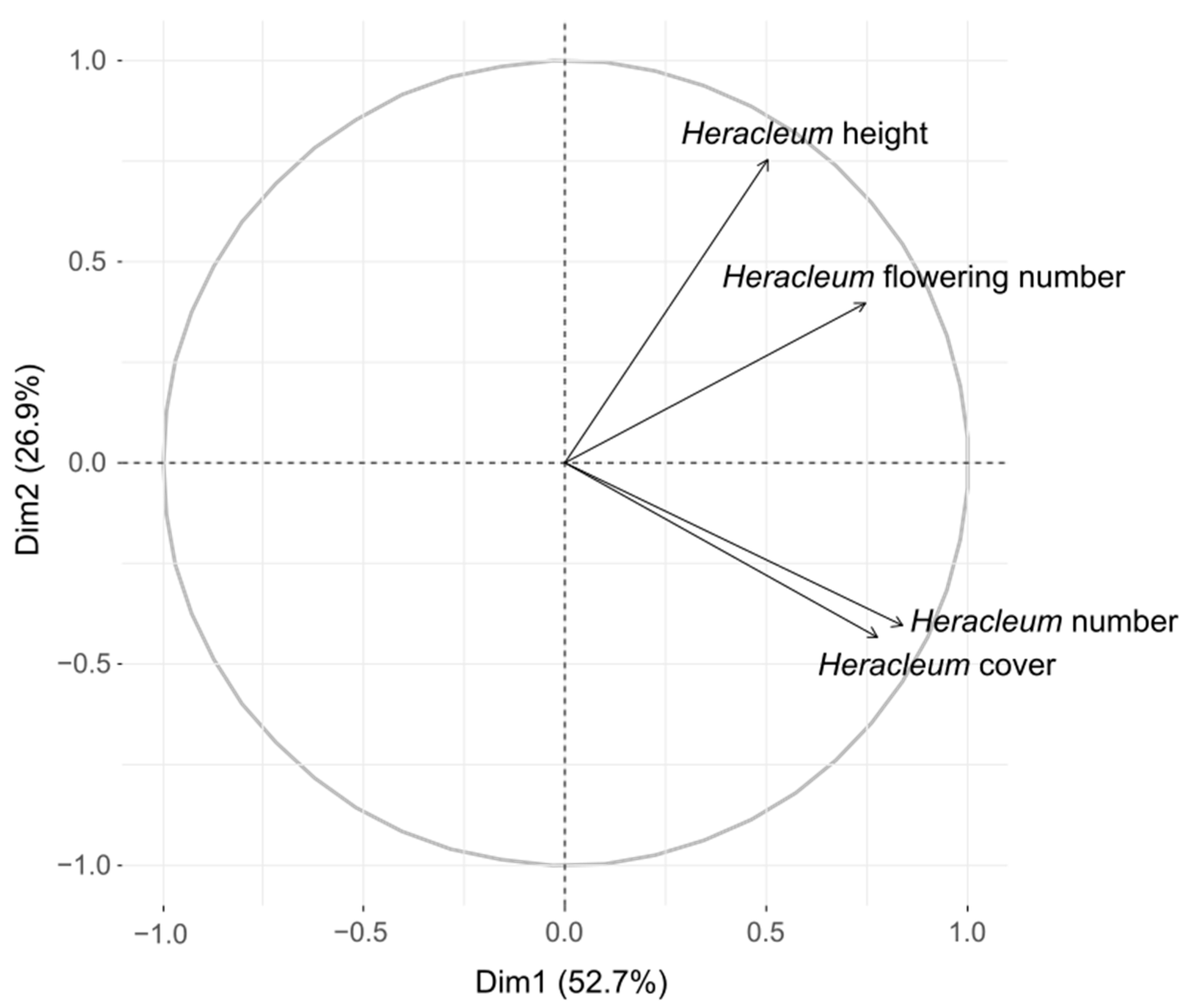
In 2019, the invaded 50 m radius plots were studied in terms of the variability of traits of Caucasian hogweeds, which were as follows: number and cover of invaders in plots, the maximum height of invaders in plots, as well as the number of flowering ones in plots. On each plot, the traits of hogweeds were recorded on three dates selected according to their phenology: first field visit: 25 April–20 May 2019 (invaders were visible in the field), second field visit: 21 May–11 June 2019 (invaders’ full development of green parts), 3rd field visit: 12 June–15 July 2019 (invaders had flowers), with a minimum interval of 14 days between field visits at a particular plot. Each field visit was treated independently because on the second and third ones, new hogweeds were growing at different periods, and the number and cover of non-flowering invaders did not give a basis to predict how many of them would bloom and what height they would reach. However, since these values were generally correlated with each other (the more severe invasion, the greater the development of the traits), I used principal component analysis (PCA) run in R 4.0.4 [33] using “factoextra” package [34] on the correlation matrix of these four traits to compute one collective Heracleum PC. Dim1 explained 52.7% of the variance and was strongly positively correlated with all measured traits (Figure 3).
Habitats on 50 m radius plots were assigned to one of the following categories: meadow (i.e., meadows or pastures from the Molinio-Arrhenatheretea class sometimes with an admixture of vegetation belonging to wetland Phragmitetea class or xerothermic plants from the Festuco-Brometea class), forest (i.e., deciduous forests of the Querco-Fagetea class including a mature form of riparian and floodplain forests of the Alnetea glutinosae class, coniferous forests of Vaccinio-Piceetea class, as well as mature form of riverine willow stand of the Salicetea purpureae class), bushwood (bushes including a young form of Alnetea glutinosae riparian and floodplain forests, as well as a young form of riverine willow stand of the Salicetea purpureae class), forest ecotone (parts of forests belonging to Querco-Fagetea, Vaccinio-Piceetea, and Alnetea glutinosae classes, in which the invaded areas were in the edges partially located in open forest glades or along rivers with Salicetea purpurae and Phragmitetea vegetation), meadow ecotone (Molinio-Arrhenatheretea meadows with an admixture of Phragmitetea vegetation and bushes classified as Salicetea purpureae class or initial and very young stage of Alnetea glutinosae forest).
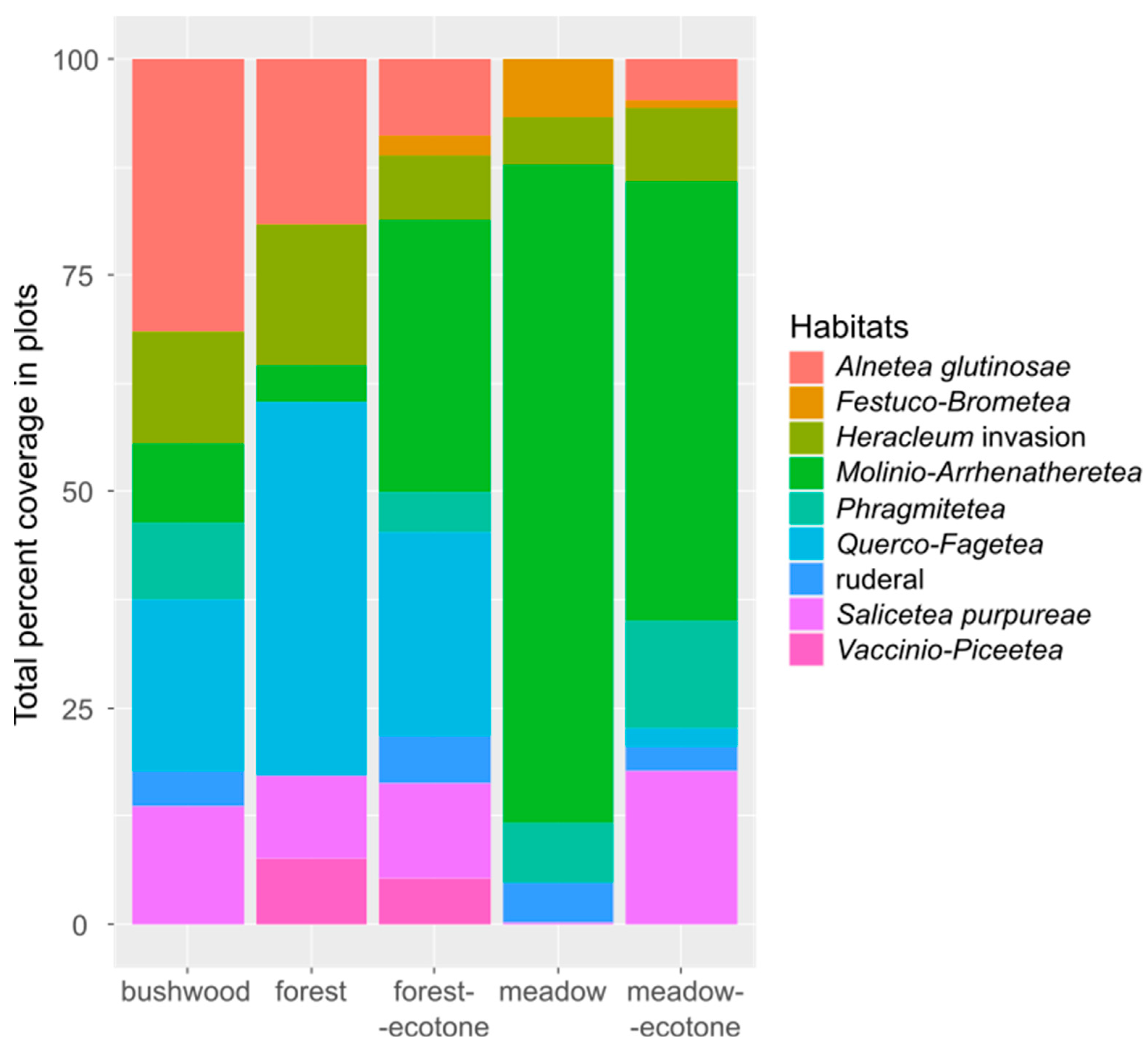
In the case of habitats classified as meadow (9 plots), forest (9 plots), or bushwood (11 plots), the plot had to be covered with the assigned plant communities on at least 80% of the area, including the invaded area, if it constituted a fragment of a meadow (Figure 1d) or forest (Figure 1a), respectively. In the case of ecotone habitats (i.e., edges), the location of the invaders was decisive. If the invasion patch was mostly in the forest (i.e., forest ecotone, 11 plots), the plot was set there, but usually, the forest was too small to cover the entire plot, so a maximum of 40% of the plot had other habitats (i.e., bushes, meadows, ruderal areas). If the invasion patch was mostly in the meadow area (i.e., meadow ecotone, 12 plots), but it was too small to cover the entire plot, a maximum of 40% of its area was in other habitats—i.e., ruderal areas, bushes, very initial and young stages of forest. To illustrate the share of individual plant communities in plots from five categories (bushwood, forest, meadow, forest ecotone, meadow ecotone), their areas in all plots separately from each category were summed up and used to calculate the percentage frequencies (Figure 4).
Based on habitat data collected from plots in June and July of the year 2021, a satellite map in Google Maps was used to measure the areas (in tenths of square meters, then summarized and expressed in hectares) of nine types of habitats: meadows, ruderal ones, built areas (houses, gazebos, apiaries, energy stations), agriculture (i.e., croplands, including both used and abandoned lands), forests, bushes, roads, water bodies (stream, river, pond), as well as the invasion of Caucasian hogweeds. The area of invasion on a given plot was subtracted from the area of other habitats, i.e., no invasion patch was included as invaded and uninvaded habitat. It was assumed that the invasion was influenced by space co-occurrence of the following habitats: meadows, ruderal areas, agriculture areas, forests, and bushes, while buildings and water bodies occurred independently of the others. PCA analysis using the “factoextra” package [34] was on the correlation matrix of five main and related habitat types. Dim1 explained 32.3% of habitat variance and expressed a gradient from agriculture (the positive part of Dim1) to meadow areas (the negative part of Dim1). Dim2 explained 29.2% of the variance reflecting a gradient from forests and bushes (most important contributors) at the negative part of Dim2 to meadows and agriculture at the positive part of Dim2. Dim3 explained 24% of habitat variance and reflected a gradient from ruderal areas (positive part of Dim3) to forests (negative part of Dim3)—both dominating contributors of Dim3. Dim4 explained 13.3% of the variance and described a gradient from bushes at the negative part of Dim4 (its highest contributor) to ruderal areas at its positive part. These clarified values used in analyses as habitat gradients were assumed as expressing the meadow–agriculture relationship (Dim1, hereafter “PC1”—see Figure 1b in the front), overgrown–open relationship (Dim2, hereafter “PC2”—see Figure 1b in the back), forest–ruderal relationship (Dim3, hereafter “PC3”), and bushes–ruderal areas (Dim4, hereafter “PC4”—see Figure 1d).

2.4. Statistical Analysis

All statistical analyses were performed using the software R 4.0.4 [33]. To explore the impacts of habitats from five categories and the areas of plant communities on the performance of invaders’ traits in 50 m radius plots, the “vegan” package [35] was chosen and the relationships were tested via a detrended correspondence analysis (DCA). To avoid pseudoreplication (areas of plant communities were measured once, and the traits measurements were repeated three times on constant plots, so they were not independent), the invasiveness traits measurements used in DCA were based only on the results of third field visits with maximal trait performance. The distribution of study plots (site scores) was illustrated in the ordination plot, and the invasiveness traits were treated as species scores rescaled using the decorana function. The impact of habitat categories or areas of plant communities on traits in plots was tested using the envfit command. The extent of areas of plant communities that were statistically significant in their impacts on traits, as well as five categories of habitats, were expressed by the “polygon” option and scaled to site scores. The relative strengths of the DCA axes were given as eigenvalues (lambda, λ).
Using the Shapiro–Wilk test, it was shown that Heracleum PC was not normally distributed (W = 0.872, p < 0.001). Therefore, I chose the “bestNormalize” package [36,37] proposing the most correct data transformation to a distribution close to the normal one according to the package calculations (in this case, Yeo–Johnson transformation). To investigate whether and which habitats favored the maximal development of invasiveness traits of Caucasian hogweeds (in the meaning of one collective PC), I used a linear mixed model prepared in the “glmmTMB” package [38]. The transformed Heracleum PC was the respective dependent variable in linear mixed model LMM with Gaussian distribution and identity link function. The fit of the model was the maximum likelihood, while “visit ID” (1, 2, or 3—see above) was treated as the random effect. The single nominal predictor was the habitat, in which the respective plot was located (bushwood, forest, forest ecotone, meadow, meadow ecotone)
To assess which habitat gradients (PC1–PC4 scores, see above) influenced the probability of Caucasian hogweeds’ presence, I used a generalized linear mixed model. Before preparation of the final model, the fit of the designed one with all habitat variables was tested using the “glmulti” package [39] where the dependent variable (the presence of invasion) had binomial distribution and logit link function, the “site ID” (i.e., identification of the site where four connected study plots were set: invaded vs. control, and their two references) was used as the random effect, while four habitat gradients expressed as PC scores were used as predictors. Based on Akaike’s information criterion (AIC), it was chosen the best-fitted version of the model. The variance inflation factor (VIF) analysis in the “performance” package [40] and the correlation matrix of predictors were run to identify if any of the collinear predictor variables should be removed from the analysis (VIF < 5 and correlation values r < 0.9 were treated as low).
The final generalized linear mixed model GLMM assessing the impacts of habitat gradients on the probability of invaders’ presence was designed in the “lme4” package [41], using the glmer function. This model allowed investigation of whether the Caucasian hogweeds occurred between particular transforming habitats if one of them showed a decreasing area, while the second one was increasing at the same time. The dependent variable (1—the presence of invasion, 0—the absence of invasion) had a binomial distribution and a logit link function; the fit of the model was a maximum likelihood, while “site ID” was the random effect. The predictors were three habitat gradients from the best-fitted version of the model expressed as PC scores.

3. Results

Comparing three field visits from the year 2019, the mean hogweed coverage in the plot increased by approx. 5% between the first and second field visit and 1% during the third field visit, while the mean number of plants remained similar. The flowering of hogweeds was recorded on 41 plots (78.8% of Heracleum ones). The mean number of flowering invading plants in the plot was 94 (on average 51.4% of the invaders present in the study plot, ranging from 0 to 600—Table 1), while the remained ones were hogweeds developing only green leaf rosettes.
Considering the summarized areas of N = 52 plots with a 50 m radius, the highest value 14.08 ha (i.e., 34.3%) had meadows of the Molinio-Arrhenatheretea class and forest belonging to Querco-Fagetea (7.03 ha and 17.1%). The remained plant communities had the following areas: Alnetea glutinosae 5.34 ha (i.e., 13%), Salicetea purpureae 4.53 ha (11%), Phragmitetea 2.86 ha (7%), ruderal areas 1.44 ha (3.5%), Vaccinio-Piceetea 0.99 ha (2.4%) and Festuco-Brometea 0.77 ha (1.9%). The number of invaders in plots was highest in meadows and meadow ecotone habitats, and the number of flowering specimens was lowest in overgrown habitats (Table 2, Figure 5).
DCA (Figure 5) showed that the meadow area from the Molinio-Arrhenatheretea class and meadow habitat in general significantly impacted Heracleum traits (i.e., number, height, cover) favoring their homogeneously good performance. Moreover, the area of the Alnetea glutinosae forest community favored higher cover and many hogweeds. It was confirmed by the width of the polygon in the positive part of DCA2 reflecting these traits, and in the case of categorized habitats, most of the areas of forest and bushwood with the highest areas of Alnetea glutinosae were in the positive part of DCA2 (Figure 5). The other areas of plant communities did not impact individual traits. The low impact of particular habitats on traits’ performance (Figure 5) confirmed the need for analysis on Heracleum PC.
Based on research on 50 m radius plots in 2019, it was shown that Caucasian hogweeds generally achieved the best performance of joint invasiveness traits (i.e., number, cover, height, flowering number) in meadows and forests compared to bushwoods and ecotone habitats (Table 3, Figure 6).
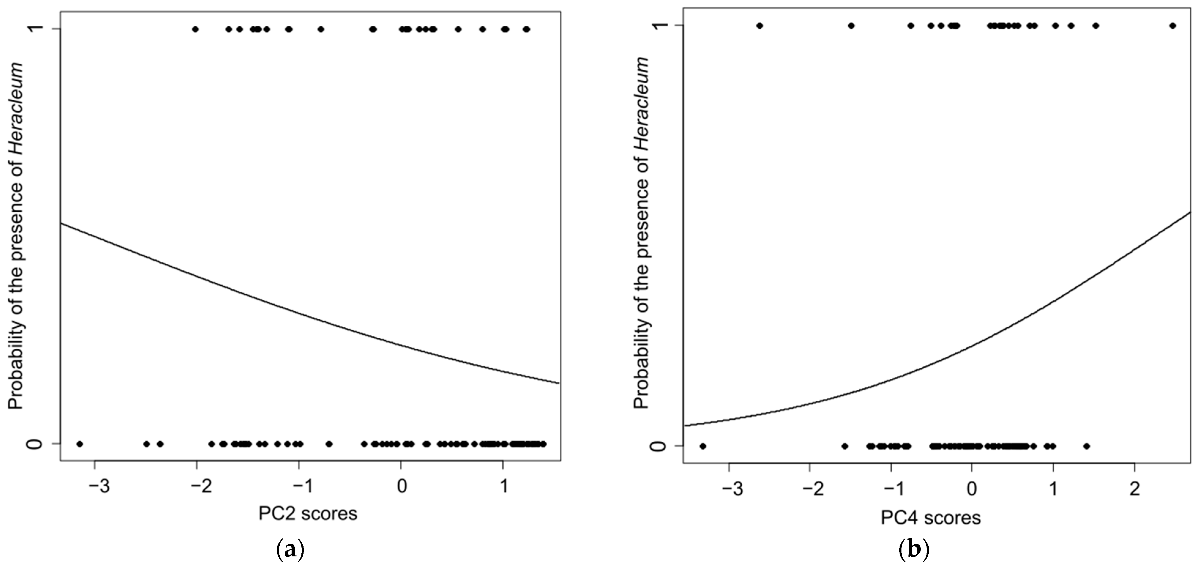
Based on research on 100 m radius plots in 2021, it turned out that the occurrence of Caucasian hogweeds invasion was more likely with increasing overgrown areas with a simultaneous decrease in the open areas, as well as in the increasing ruderal areas with a simultaneous decrease in bushes (Table 4, Figure 7). The PC2 and PC4 scores were not correlated (Pearson correlation coefficient: r = –0.085, df = 110, p = 0.376). In connection with PC2 scores, open areas on plots were significantly negatively correlated with overgrown areas (r = –0.895, df = 110, p < 0.001), while the correlation between bushes and ruderal areas (PC4) was close to the significance and positive but low (r = 0.206, df = 88, p = 0.051).

4. Discussion

This study showed that the probability of the Caucasian hogweeds occurrence was highest in places with transformations between habitats. First, open areas (i.e., meadows and agriculture) were overgrowing with trees and shrubs, or these two habitat types coexisted due to the land management system. Secondly, ruderal areas appeared as the size of the bush area decreased. In both cases, there was competition for space between edge plant communities. The presence of invaders at such points can be due to the competition for resources in disturbed habitats that weakens native organisms while favoring low-demanding ones such as invasive plants. Although under low resource availability, both native and alien species are comparably competitive [6], edge habitats may sometimes contain increased resources [22], and, therefore, alien plants become more competitive and successful [6] in such points. In the case of open–overgrowing gradient, it was common in the area—meadows and agricultural areas accounted for a total of 223.46 ha on 112 plots (63.5%), while forests and bushes—87.87 ha (25%) and most often as an overgrown admixture in the mosaic of an agricultural landscape. The significantly negative correlation found between open and overgrown habitats does not illustrate the relationship between them. This relationship was not gradual across all plots and the correlation reflected the varying proportions between open and overgrown areas measured in constant area units. Many local conditions made the relationship between these habitats non-linear. The greater diversity of habitats and more frequent contacts between open and overgrown areas (i.e., habitat edges) were conducive to the formation of abandoned niches with the benefit of facilitating the spread of invasive plants.
The gradient between bushes and ruderal areas needs emphasis because it was rarer in the studied landscape. The ruderal area accounted for only 9.3 ha, i.e., 2.6% of all 112 surveyed plots, of which a quarter contained invaders. This can be interpreted in such a way that ruderal habitats of anthropogenic origin are a type of disturbance favoring the creation of new sites for the studied plant invaders. This might be related to the invasion vector, which was a human. Such biotic filters that constrain the population size of invaders (i.e., the number of their locations) someday may be most important. They interact with environmental conditions, species traits, and continued propagule pressure from source regions. Biotic filters can be vectors of invasion, but also barriers created by the actions or presence of living organisms. While biotic filters will not necessarily prevent the germination of seeds or the spread of invasive plants, these filters can affect their survival, growth, and reproduction [22]. Ruderal areas cannot be, therefore, underestimated in landscapes with the problem of plant invasion. The presented study confirmed the negative effect of a ruderal area previously shown by other research [13,18,20,42]. Since the correlation between the area of bushes and ruderal areas turned out to be close to significant and positive, it can be suspected that both these habitats occupied similar spaces, but invaders appeared when ruderal vegetation began to prevail over bushes. Bushes could be lost through a variety of processes—intentional land management, development of herbaceous ruderal vegetation, or failure of young bush seedlings competing with more diverse herbaceous plants.
Caucasian hogweeds showed the best performance of their invasiveness traits in continuous habitats—meadows and forests. As in classical ecology, they probably won the competition for resources with other plants—in the forest undergrowth and herbaceous meadow vegetation. Without disturbances of anthropogenic origin and obstacles to the dissemination of propagules, they could invest maximum resources in the development of their organisms—height, leaves, and inflorescences. It also turned out that particular plant communities impacted the performance of individual traits, i.e., the area of meadow belonging to Molinio-Arrhenatheretea class favored good performance of Heracleum number, height, and cover. Moreover, the area of the Alnetea glutinosae forest community favored higher cover of many hogweeds. The number of invaders in plots was highest in the meadow and meadow ecotone ones, while the number of flowering specimens was lowest in overgrown habitats. In another study, native species that were more similar to invasive plants in multivariate space were excluded more, however, this was not the case in the meadow habitat. This suggests that some plant invaders alter communities uniquely in each habitat. This filtering process could cause a non-random reduction in native species’ abundances [43]. The selective action of invading species on native communities could also be the reason why Caucasian hogweeds more visibly won the competition with native plants in meadow habitats than in overgrown ones. Here, meadow native plants were the most similar to herbaceous weeds and therefore lost the fastest near the invaders. The result showing the good performance of Heracleum traits in forests may result from success in competition with native herbaceous species in the undergrowth.
The approach that distinguishes the mere quantitative fact of the presence of invaders from the quality and severity of invaded areas was rarely taken into account by researchers. This is quite a significant oversight because traits related to the relative competitive ability of invasive species determine the severity of invasion impacts [44]. The best performance of invasiveness traits in homogeneous habitats and the fact that invaders win the competition with natives in resource-rich areas contribute to the most severely invaded patches in continuous habitats, as shown by the presented research. On the other hand, it is important to explain why in some, e.g., continuous and overgrown habitats, there are not as much of negative invasion effects as in others, such as open habitats [20]. This may be due to the varied performances of different traits in specific plant communities. For example, species invasiveness can be expressed as its percentage frequency, although most of the habitats are colonized by a few alien species, except for some disturbed and synanthropic habitats. The number of alien species occurring in a given habitat does not necessarily relate to the severity of the impact of invasion in that habitat. Some habitats are invaded by few (or single) species, which attain a high cover, transforming the whole ecosystem [45], which, contrary to appearances, is tantamount to a severe invasion, even if the measurements do not indicate this. Habitat conditions in a given plant community may also influence the development of invasiveness traits in basic physical processes, such as access to light and water. This explains the relatively small number of flowering hogweeds in overgrown habitats found in this research. In another study, alien species growing in urban areas tended to show trait values associated with drought tolerance, including higher leaf length-to-width ratio, greater leaf thickness, higher leaf dry matter content, and lower specific leaf area [46]. The mesic forest stands had the greatest invasive plant richness, frequency, and abundance, while the mature forests showed no change in native species abundance in response to invasion [47]. All these conditions mean that the obtained results regarding the performance of particular invasiveness traits in various habitats must be treated with caution. It is better to study the spatial co-evolution of correlated traits (such as here: Heracleum PC) than one selected trait.
The invasion of plant species is among the most important components of global environmental change. Identifying the stage at which an invasion fails may allow us to understand the interaction of invasion filters with invasion character (e.g., number of introduction points), species traits, and ecosystem characteristics. To establish, an invader must colonize a habitat and perform self-sustaining, expanding populations [22]. The landscape heterogeneity includes both environmental (geomorphology, resource availability, and soil types) and biotic (often measured as beta diversity) heterogeneity [22], which means that the effects resulting from the influence of habitat gradients on invasions do not have to be directly proportional to the effects that invaders performing in these gradients may have on the success of settlement of habitats by many organisms. Habitat selection indicates whether specific habitats are positively or negatively selected by a given species (in this case: invader), i.e., occupied more or less than expected based on the level of habitat availability [12]. For example, the significant role of ruderal habitats demonstrated in this study indicates that an extremely disturbed anthropogenic habitat can cause a lot of damage to the environment if it is inhabited by invaders. An establishment may last longer than colonization and occurs on a slightly larger spatial scale. Small subpopulations may be tightly linked through dispersal [48]. This means that in the case of invading species, both components of habitat selection complement each other—colonization of small, disturbed habitats and best performance in homogeneous resource-rich habitats. Selection gradients for pre-emptive habitat selection are steeper than those for passive dispersal and yield an advantage that increases with population density [49]. Creating numerous anthropogenic invasion openings close to continuous habitats is particularly threatening to the environment.
Habitat selection similar to that of invaders may be in some current native organisms, which may one day enter the expansion phase due to changes in the ranges of habitats necessary for them. For example, such organisms can be found among pioneer species that are successful in succession. Habitat selection depends critically on population density and the frequency of alternative strategies: they are evolutionary games [49]. Global changes will involve numerous disturbances in habitats, so all natives that function well in such conditions have the potential to become future invaders. Using trait-based frameworks leads to a better understanding and prediction of invasion impacts. This novel framework can be used in restoration practices to understand how invasion impacts communities and to reassemble communities after invasive species management [43]. Identifying specific traits of species that distinguish among successful invaders most likely to result in more severe impacts can help with planning more effective interventions [44]. Understanding the transition from the non-invasive naturalized to the invasive stage of the plant invasion process is important, particularly for those species that recently established in a new habitat. The data concerning the probability of occurrence, such as those used in this study, accurately investigate the adaptability of a given species to different habitats and its relative frequency but they are less suitable for assessing the invasiveness of individual alien species.

5. Conclusions

This study showed that a mosaic of habitats containing transformations of anthropogenic origin (i.e., favoring ruderal areas) or spontaneous ones and fragmenting habitats (i.e., overgrowing the open areas) favored the occurrence of plant invasion. As predicted, the invaders with the best performance of invasiveness traits were found in resource-rich homogeneous habitats, meadows, and forests, not in the edge (i.e., ecotone) habitats. These are two aspects of invaders’ habitat selection, not separated so far. The best performance of invasiveness traits in homogeneous habitats was connected with the most severely invaded patches. Because invaders must first colonize a habitat and, secondly, perform self-sustaining, expanding populations, anthropogenic openings for those plants can be particularly threatening close to continuous habitats. It can be expected that some currently non-invasive organisms presenting similar duality in habitat selection may one day enter the expansion phase in the more intensively modified habitats.

Funding

During the preparation of the manuscript, the author was supported by statutory funds from the Institute of Systematics and Evolution of Animals, Polish Academy of Sciences.

Institutional Review Board Statement

Not Applicable.

Data Availability Statement

Data can be available from the author upon a reasonable request.

Conflicts of Interest

The author declares no conflict of interest.

References

  1. Vitousek, P.M.; D’Antonio, C.M.; Loope, L.L.; Westbrooks, R. Biological invasions as global environmental change. Am. Sci. 1996, 84, 468–478. [Google Scholar]
  2. Early, R.; Bradley, B.A.; Dukes, J.S.; Lawler, J.J.; Olden, J.D.; Blumenthal, D.M.; Gonzalez, P.; Grosholz, E.D.; Ibañez, I.; Miller, L.P.; et al. Global threats from invasive alien species in the twenty-first century and national response capacities. Nat. Commun. 2016, 7, 12485. [Google Scholar] [CrossRef] [PubMed] [Green Version]
  3. Rumlerová, Z.; Vilà, M.; Pergl, J.; Nentwig, W.; Pyšek, P. Scoring environmental and socioeconomic impacts of alien plants invasive in Europe. Biol. Invasions 2016, 18, 3697–3711. [Google Scholar] [CrossRef]
  4. Grzędzicka, E.; Hanzelka, J.; Reif, J. The area of Caucasian hogweeds’ invasion impacts bird responses to habitats in a heterogeneous landscape. Ecol. Indic. 2022, 141, 109082. [Google Scholar] [CrossRef]
  5. Grainger, T.N.; Levine, J.M.; Gilbert, B. The invasion criterion: A common currency for ecological research. Trends Ecol. Evol. 2019, 34, 925–935. [Google Scholar] [CrossRef]
  6. Zhang, Z.; Liu, Y.; Hardrath, A.; Jin, H.; van Kleuen, M. Increases in multiple resources promote competitive ability of naturalized non-native plants. Commun. Biol. 2022, 5, 1150. [Google Scholar] [CrossRef]
  7. Arroyo-Esquivel, J.; Hastings, A. Spatial dynamics and spread of ecosystem engineers: Two patch analysis. Bull. Math. Biol. 2020, 82, 149. [Google Scholar] [CrossRef]
  8. Bazzaz, F.A. Habitat selection in plants. Am. Nat. 1991, 137, 116–130. [Google Scholar] [CrossRef]
  9. Gersani, M.; Abramsky, Z.; Falik, O. Density-dependent habitat selection in plants. Evol. Ecol. 1998, 12, 223–234. [Google Scholar] [CrossRef]
  10. Pyšek, P.; Richardson, D.M.; Rejmánek, M.; Webster, G.L.; Williamson, M.; Kirschner, J. Alien plants in checklists and floras: Towards better communication between taxonomists and ecologists. Taxon 2004, 53, 131–143. [Google Scholar] [CrossRef]
  11. Weiner, J.; Mallory, E.B.; Kennedy, C. Growth and variability in crowded and uncrowded populations of dwarf marigolds (Tagetes patula). Ann. Bot. 1990, 65, 513–524. [Google Scholar] [CrossRef]
  12. Carranza, M.L.; Ricotta, C.; Carboni, M.; Acosta, A.T.R. Habitat selection by invasive alien plants: A bootstrap approach. Preslia 2011, 83, 529–536. [Google Scholar]
  13. Chytrý, M.; Jarošík, V.; Pyšek, P.; Hájek, O.; Knollová, I.; Tichý, L.; Danihelka, J. Separating habitat invasibility by alien plants from the actual level of invasion. Ecology 2008, 89, 1541–1553. [Google Scholar] [CrossRef] [PubMed] [Green Version]
  14. Essl, F.; Dullinger, S.; Kleinbauer, I. Changes in the spatio-temporal patterns and habitat preferences of Ambrosia artemisiifolia during its invasion of Austria. Preslia 2009, 81, 119–133. [Google Scholar]
  15. Goldstein, J.; Park, J.; Haran, M.; Liebhold, A.; Bjørnstad, O.N. Quantifying spatio-temporal variation of invasion spread. Proc. R. Soc. B 2019, 286, 20182294. [Google Scholar] [CrossRef] [PubMed] [Green Version]
  16. Lodge, D.M. Biological invasions: Lessons from ecology. Trends Ecol. Evol. 1993, 8, 133–136. [Google Scholar] [CrossRef]
  17. Lear, L.; Padfield, D.; Inamine, H.; Shea, K.; Buckling, A. Disturbance-mediated invasions are dependent on community resource abundance. Ecology 2022, 103, e3728. [Google Scholar] [CrossRef] [PubMed]
  18. Vázquez-Reyes, L.D.; Paz-Hernández, H.; Godínez-Álvarez, H.O.; del Coro Arizmendi, M.; Navarro-Sigüenza, A.G. Trait shifts in bird communities from primary forest to human settlements in Mexican seasonal forests. Are there ruderal birds? Perspect. Ecol. Conserv. 2022, 20, 117–125. [Google Scholar] [CrossRef]
  19. Liu, K.; Liang, T.; Qiang, W.; Du, G.; Baskin, J.M.; Baskin, C.C.; Bu, H.; Yang, H.; Xiao, S. Changes in seed germination strategy along the successional gradient from abandoned cropland to climax grassland in a subalpine meadow and some implications for rangeland restoration. Agric. Ecosyst. Environ. 2020, 289, 106746. [Google Scholar] [CrossRef]
  20. Grzędzicka, E. Impact of invasive weeds on the diversity and dissimilarity of bird communities in forested areas. Diversity 2022, 14, 229. [Google Scholar] [CrossRef]
  21. Lapin, K.; Oettel, J.; Steiner, H.; Langmaier, M.; Sustic, D.; Starlinger, F.; Kindermann, G.; Frank, G. Invasive alien plant species in unmanaged forest reserves, Austria. NeoBiota 2019, 48, 71–96. [Google Scholar] [CrossRef] [Green Version]
  22. Theoharides, K.A.; Dukes, J.S. Plant invasion across space and time: Factors affecting nonindigenous species success during four stages of invasion. New Phytol. 2007, 176, 256–273. [Google Scholar] [CrossRef] [PubMed]
  23. Trombulak, S.C.; Frissell, C.A. Review of ecological effects of roads on terrestrial and aquatic communities. Conserv. Biol. 2000, 14, 18–30. [Google Scholar] [CrossRef] [Green Version]
  24. Fenner, M.; Thompson, K. The Ecology of Seeds; Cambridge University Press: Cambridge, UK, 2005. [Google Scholar]
  25. Alpert, P.; Bone, E.; Holzapfel, C. Invasiveness, invasibility and the role of environmental stress in the spread of non-native plants. Perspect. Plant Ecol. 2000, 3, 52–66. [Google Scholar] [CrossRef] [Green Version]
  26. Wang, C.; Cheng, H.; Wei, M.; Wang, S.; Wu, B.; Du, D. Plant height and leaf size: Which one is more important in affecting the successful invasion of Solidago canadensis and Conyza canadensis in urban ecosystems? Urban For. Urban Green. 2021, 59, 127033. [Google Scholar] [CrossRef]
  27. Catford, J.A.; Jansson, R.; Nilsson, C. Reducing redundancy in invasion ecology by integrating hypotheses into a single theoretical framework. Divers. Distrib. 2009, 15, 22–40. [Google Scholar] [CrossRef] [Green Version]
  28. Ricciardi, A.; Hoopes, M.F.; Marchetti, M.P.; Lockwood, J.L. Progress toward understanding the ecological impacts of nonnative species. Ecol. Monogr. 2013, 83, 263–282. [Google Scholar] [CrossRef] [Green Version]
  29. Tomasetto, F.; Duncan, R.P.; Hulme, P.E. Environmental gradients shift the direction of the relationship between native and alien plant species richness. Divers. Distrib. 2013, 19, 49–59. [Google Scholar] [CrossRef]
  30. Grzędzicka, E. Invasion of the Giant Hogweed and the Sosnowsky’s Hogweed as a multidisciplinary problem with unknown future—A review. Earth 2022, 3, 287–312. [Google Scholar] [CrossRef]
  31. Pearson, D.E.; Ortega, Y.K.; Runyon, J.B.; Butler, J.C. Secondary invasion: The bane of weed management. Biol. Conserv. 2016, 197, 8–17. [Google Scholar] [CrossRef] [Green Version]
  32. Neve, P.; Barney, J.N.; Buckley, Y.; Cousens, R.D.; Graham, S.; Jordan, N.R.; Lawton-Rauh, A.; Liebman, M.; Mesgaran, M.B.; Schut, M.; et al. Reviewing research priorities in weed ecology, evolution and management: A horizon scan. Weed Res. 2018, 58, 250–258. [Google Scholar] [CrossRef] [PubMed] [Green Version]
  33. R Core Team. R. A Language and Environment for Statistical Computing; R Foundation for Statistical Computing: Vienna, Austria, 2021; Available online: https://www.R-project.org/ (accessed on 15 February 2021).
  34. Kassambara, A.; Mundt, F. factoextra: Extract and Visualize the Results of Multivariate Data Analyses. R Package Version 1.0.7. 2020. Available online: https://CRAN.R-project.org/package=factoextra/ (accessed on 15 February 2021).
  35. Oksanen, J.; Blanchet, F.G.; Friendly, M.; Kindt, R.; Legendre, P.; McGlinn, D.; Minchin, P.R.; O’Hara, R.B.; Simpson, G.L.; Solymos, P.; et al. vegan: Community Ecology Package. R Package Version 2.5-7. 2020. Available online: https://CRAN.R-project.org/package=vegan/ (accessed on 27 December 2021).
  36. Peterson, R.A.; Cavanaugh, J.E. Ordered quantile normalization: A semiparametric transformation built for the cross-validation era. J. Appl. Stat. 2020, 47, 2312–2327. [Google Scholar] [CrossRef] [PubMed]
  37. Peterson, R.A. Finding Optimal Normalizing Transformations via bestNormalize. R J. 2021, 13, 310–329. [Google Scholar] [CrossRef]
  38. Brooks, M.E.; Kristensen, K.; van Benthem, K.J.; Magnusson, A.; Berg, C.W.; Nielsen, A.; Skaug, H.J.; Maechler, M.; Bolker, B.M. glmmTMB balances speed and flexibility among packages for zero-inflated generalized linear mixed modeling. R J. 2017, 9, 378–400. [Google Scholar] [CrossRef] [Green Version]
  39. Calcagno, V. glmulti: Model Selection and Multimodel Inference Made Easy. R Package Version 1.0.8. 2020. Available online: https://CRAN.R-project.org/package=glmulti/ (accessed on 14 July 2022).
  40. Lüdecke, D.; Makowski, D.; Waggoner, P.; Patil, I. performance: Assessment of Regression Models Performance. 2020. Available online: https://CRAN.R-project.org/package=performance/ (accessed on 17 March 2021).
  41. Bates, D.; Maechler, M.; Bolker, B.; Walker, S. Fitting linear mixed-effects models using lme4. J. Stat. Softw. 2015, 67, 1–48. [Google Scholar] [CrossRef]
  42. Grzędzicka, E. Assessing the role of invasive weeds in the impact of successional habitats on the bird assemblage in overgrowing agriculture. J. Nat. Conserv. 2022, 72, 126352. [Google Scholar] [CrossRef]
  43. Sodhi, D.S.; Livingstone, S.W.; Carboni, M.; Cadotte, M.W. Plant invasion alters trait composition and diversity across habitats. Ecol. Evol. 2019, 9, 6199–6210. [Google Scholar] [CrossRef]
  44. Ni, M.; Deane, D.C.; Li, S.; Wu, Y.; Sui, X.; Xu, H.; Chu, C.; He, F.; Fang, S. Invasion success and impacts depend on different characteristics in non-native plants. Divers. Distrib. 2021, 27, 1194–1207. [Google Scholar] [CrossRef]
  45. Guarino, R.; Chytrý, M.; Attorre, F.; Landucci, F.; Marcenò, C. Alien plant invasions in Mediterranean habitats: An assessment for Sicily. Biol. Invasions 2021, 23, 3091–3107. [Google Scholar] [CrossRef]
  46. Ariori, C.; Aiello-Lammens, M.E.; Silander, J.A. Plant invasion along an urban-to-rural gradient in northeast Connecticut. J. Urban Ecol. 2017, 3, 1–13. [Google Scholar] [CrossRef] [Green Version]
  47. Huebner, C.D. Patterns of invasive plant abundance in disturbed versus undisturbed forests within three land types over 16 years. Divers. Distrib. 2021, 27, 130–143. [Google Scholar] [CrossRef]
  48. Melbourne, B.A.; Cornell, H.A.; Davies, K.F.; Dugaw, C.J.; Elmendorf, S.; Freestone, A.L.; Hall, R.J.; Harrison, S.; Hastings, A.; Holland, M.; et al. Invasion in a heterogeneous world: Resistance, coexistence or hostile takeover? Ecol. Lett. 2007, 10, 77–94. [Google Scholar] [CrossRef] [PubMed]
  49. Morris, D.W.; Lundberg, P.; Brown, J.S. On strategies of plant behaviour: Evolutionary games of habitat selection, defence, and foraging. Evol. Ecol. Res. 2016, 17, 619–636. [Google Scholar]
Figure 1. Examples of habitats selected by Caucasian hogweeds (i.e., Heracleum sosnowskyi, Heracleum mantegazzianum): (a) riverine willow stand; (b) an agricultural landscape with a developed invaded patch in the meadow part in the front of the photo and invaders on the edge of the forest with the ruderal area and cropland in the back; (c) an example of hogweeds rebuilding after habitat disturbance (i.e., mowing of the meadow) much faster than native vegetation; (d) a patch of Caucasian hogweeds in the meadow with an admixture of ruderal area. Photos by: E. Grzędzicka (June–July 2022, South-Eastern Poland).
Diversity 15 00333 g001
Figure 2. Map of the study plots with Caucasian hogweeds (N = 52 from 2019, N = 28 from 2021) in South-Eastern Poland. Free background source: geoportal.gov.pl (accessed on 19 January 2022).
Diversity 15 00333 g002
Figure 3. Principal component analysis PCA showing the relationships between invasiveness traits of Caucasian hogweeds in the 50 m radius study plots.
Diversity 15 00333 g003
Figure 4. Total percent coverage of various plant communities on 50 m radius plots classified into five categories (bushwood, forest, forest ecotone, meadow, meadow ecotone).
Diversity 15 00333 g004
Figure 5. The relationships between habitats from five categories (above) or plant communities (below; marked in bold and polygon if significant) and invasiveness traits of Caucasian hogweeds measured during the third field visit in the 50 m radius study plots.
Diversity 15 00333 g005
Figure 6. The performance of Caucasian hogweeds’ invasiveness traits in habitat categories.
Diversity 15 00333 g006
Figure 7. The probability of the presence of Caucasian hogweeds higher with increasing overgrown areas and decreasing open areas (a); and a higher probability of the invaders’ presence in the increasing ruderal areas along with a decrease in bushes (b).
Diversity 15 00333 g007
Table 1. Caucasian hogweeds’ average traits for each field inspection separately, determined within a 50 m radius circle plots; the ranges of recorded measurements on 52 plots are given in brackets.
Heracleum Traits1st Field Visit2nd Field Visit3rd Field Visit
Heracleum cover49.23% (25–90%)54.33% (25–90%)55.38% (25–90%)
Heracleum number172 (10–1000)176.5 (10–1000)183 (10–1000)
Heracleum height48.3 cm (20–100 cm)130 cm (50–150 cm)202 cm (50–250 cm)
Heracleum flowering number0094 (0–600)
Table 2. Caucasian hogweeds’ average traits from the third field visit determined within 50 m radius circle plots separately from each of the five habitat categories.
Heracleum TraitsMeadowMeadow EcotoneBushwoodForest EcotoneForest
Heracleum cover65.62%56.82%55.45%47.73%50%
Heracleum number30519711015287
Heracleum height220 cm210 cm177 cm200 cm200 cm
Heracleum flowering number179125424840
Table 3. A linear mixed model with Heracleum PC as the dependent variable and habitat category as a nominal predictor. “Count ID” was the random effect.
Habitat VariablesEstimate ± SEzp
(Intercept)−0.340 ± 0.395−0.8610.389
Forest0.763 ± 0.3292.3230.020
Forest ecotone0.099 ± 0.3120.3180.751
Meadow1.073 ± 0.3323.2310.001
Meadow ecotone0.057 ± 0.3070.1870.852
Table 4. The generalized linear mixed model with the presence or absence of invasion of Caucasian hogweeds as a binomial dependent variable and the best-fitted set of habitat gradients (PC scores) used as continuous predictors. “Site ID” was the random effect.
Habitat Gradients (PC Scores)Estimate ± SEzp
(Intercept)−1.126 ± 0.234−4.823<0.001
PC2 scores (overgrown–open)−0.491 ± 0.225−2.1820.029
PC3 scores (forest–ruderal)0.514 ± 0.2891.7810.075
PC4 scores (bushes–ruderal)0.654 ± 0.3321.9670.049
Disclaimer/Publisher’s Note: The statements, opinions and data contained in all publications are solely those of the individual author(s) and contributor(s) and not of MDPI and/or the editor(s). MDPI and/or the editor(s) disclaim responsibility for any injury to people or property resulting from any ideas, methods, instructions or products referred to in the content.