Article

Spatiotemporal Patterns in the Distribution of Albacore, Bigeye, Skipjack, and Yellowfin Tuna Species within the Exclusive Economic Zones of Tonga for the Years 2002 to 2018

1
School of Agriculture, Geography, Environment, Ocean and Natural Sciences, University of the South Pacific, Private Mail Bag, Suva 9072, Fiji
2
Fisheries Management Branch, Department of Forestry, Fisheries and the Environment, Foreshore, Cape Town 8012, South Africa
3
Department of Biological Sciences and Marine Research Institute, University of Cape Town, Cape Town 7701, South Africa
4
Heron Island Research Station, Faculty of Science, University of Queensland, Gladstone 4680, Australia
*
Authors to whom correspondence should be addressed.
Diversity 2023, 15(10), 1091; https://doi.org/10.3390/d15101091
Submission received: 9 August 2023 / Revised: 3 October 2023 / Accepted: 4 October 2023 / Published: 18 October 2023
(This article belongs to the Special Issue Marine Biodiversity and Ecosystems Management—2nd Edition)

Abstract

:
The Tongan fisheries targeting the species of albacore (Thunnus alalunga), bigeye (Thunnus obesus), skipjack (Katsuwonus pelamis), and yellowfin tuna (Thunnus albacares), comprising the main tuna catch landed, within the EEZ of Tonga is critical to the economy of Tonga. Thus, it is crucial to study the spatiotemporal pattern of their catch and the influence of environmental and physical variables, in addition to the month and year of the catch. To this end, sets of eight generalized additive models were applied to model the distribution of these four species. Selection among competing models was carried out based on k-fold cross-validation, using RMSPE prediction error as a measure of model predictive performance. The following sets of predictors were considered; sea surface temperature, sea surface chlorophyll, bottom depth, month, and year. In addition, to assess the influence of fronts, gradients in SST and Chl-a were computed and used as predictors. Catch year was the most important variable for all, except Albacore tuna, for which month was the important variable. The third most important variable was SST for albacore and bigeye tuna, whereas bottom depth was the most important variable for skipjack and yellowfin tuna. A standardized index of CPUE indicates mostly inter-annual variation in CPUE for albacore and bigeye tuna, whereas a it indicates a general increase in CPUE for skipjack and yellowfin tuna. Hotspots of albacore tuna catches are around the northern and southern edges of the exclusive economic zone and typically during the months of June to August. The bigeye tuna hotspots were concentrated on the eastern side of the islands, in waters overlying trenches; this was most obvious during the months of January to June. Skipjack tuna hotspots were near the edges of the exclusive economic zone, although it is caught in smaller amounts to the three tuna species considered and higher catch rates were observed only after 2014. For yellowfin tuna, the highest catch rates were concentrated around the islands and descending towards the southern edge of the EEZ. As part of the initiative of this study to support national optimal resource management, this study generated standardized CPUE (indices of abundance), an important input in stock assessment, and also looked into the potential influence of environmental and physical variables on the CPUE of these valuable tuna stocks within the EEZ of Tonga.

1. Introduction

Tonga is enveloped within the geographical boundary of the Western Central Pacific Ocean (WCPO) and its exclusive economic zone (EEZ) is managed by its Ministry of Fisheries with the objective of maintaining the viability of each tuna fishery through the implementation of its management policies. The most economically important tuna species in Tonga are albacore, bigeye, skipjack, and yellowfin, which account for over 95% of all tuna fisheries by annual catch and economic value. Tuna production is the largest commercial fishery in Tonga and is estimated at 2000 metric tonnes (mt) per year (approximately 17% of 30% of Tonga’s marine resource-related benefits) [1]. Longline is the main method for commercial tuna fishing, starting from the 1970s, although pole and line has also been used [1,2].
The application of satellite remote sensing oceanographic data within the geographic information system (GIS) has been identified as a tool that may improve tuna production and management outcomes [3,4]. Potential fishing zones (PFZ) have been identified in the EEZ of Madagascar, the Arabian Sea, Tropical Pacific Ocean, the north-west coast of India, and the western North Pacific Ocean, using satellite data collected from environmental parameters and oceanographic conditions [3,5,6]. As stated above, biophysical environmental parameters such as sea surface temperature (SST), chlorophyll-a (Chl-a) concentration, and water depths play an important role in influencing the spatial and temporal distributions of tuna [4,7]. Predictions of PFZs are established based on species distribution models aimed at parameterizing the environmental factors that influence the biology and habitats of the species of interest.
Studies have shown that environmental variables and oceanic conditions influence tuna presence; thus, characterizing their habitats is essential to understanding their spatial and temporal distributions [8,9,10]. Sea surface temperature and Chl-a concentration have been identified as playing a role in generating spatial and temporal distribution patterns of tuna in the WCPO [11], East Pacific Ocean [12], and the East Coast of Australia [7]. These studies have indicated that tropical and subtropical tuna prefer warm waters and are found in regions with high Chl-a concentration. In addition, it has been shown that the seasonal and annual patterns of tuna abundance are affected by SST and Chl-a and that their variability is related to ocean upwelling and El Nino events [13,14,15]. Utilization of satellite remotely sensed and fisheries data for management and assessment of tuna and using the information as basis for decision support by managers has not been carried out in Tonga [1] nor in its surrounding island countries like Fiji, Samoa, and Niue.
Chlorophyll-a plays a crucial role in determining the distribution of tuna as it serves as a primary indicator of primary productivity in the ocean, influencing the abundance and distribution of their prey species [13,16]. Hence, tuna rely on the presence of chlorophyll-a-rich areas as they indicate the presence of productive feeding grounds, which ultimately affects their migration patterns and distribution in search of optimal foraging opportunities. Sea surface chlorophyll-a gradients (chl_grad), affected by nutrient and light availability as well as oceanic currents, offer valuable insights into the distribution, abundance, and health of marine primary producers, contributing to the assessment of ecosystem productivity [17]. Sea surface temperature significantly influences tuna distribution as these species are ectothermic, meaning their body temperature is dependent on the surrounding environment [18]. Optimal temperature ranges dictate the presence and movement of tuna, with warmer waters often associated with increased abundance, as they provide favorable conditions for their metabolic activity and prey availability [19,20,21]. Conversely, deviations from the preferred temperature range can lead to shifts in tuna distribution, impacting their migration patterns and potentially reducing their availability in certain regions [13,20]. Ocean temperature in Tonga is above 18   ° C and is favorable for tropical and subtropical tuna species, which are known to have temperature preference range of ≥25 ° C [20]. Albacore, which is known to be temperate species, is also caught in Tongan waters and is known to have temperature preference range between 20   ° C   a n d   30   ° C in each hemisphere [20]. The sea surface temperature gradient (sst_grad) quantifies the speed of temperature change in the ocean over a specific distance, with higher gradients indicating faster changes and lower gradients indicating more gradual changes [22]. These gradients are influenced by factors such as solar radiation, ocean currents, and atmospheric conditions, and they significantly impact weather patterns, ocean circulation, and the distribution of marine life [23]. Bathymetry has been identified to affect catch rate of yellowfin and bigeye tuna in the Indian Ocean, with their catch per unit effort (CPUE) generally becoming higher as steep bathymetry zones become larger [24]. Hence, bathymetry may also play a role as Tonga EEZ envelops the Tonga Trench, Tonga Ridge, Tofua Arce Volcanic Front, the northern end of the Tonga Kermadec Arc and the westward region of the Lau Basin. These geologically bathypelagic features are part of the island nation’s fishing grounds and may influence its oceanic conditions such as; surface water temperature, nutrient, salt content, and mixed layer depth, which are habitats for pelagic species and fishing fleets. Bathymetry may also play a role since volcanic seamount lines run through the fishing ground and include very deep water more than 5000 m deep and very shallow seamounts and a large shelf that is about 2000 m deep.
Apex predators in the marine environment, including tuna, are shown to exploit frontal zones; thus, for both SST and Chl-a, frontal gradients were computed and used to model the distribution of the four tuna species [25,26]. Although the range of species distribution models can be used for the purpose of the current project, generalized additive models (GAMs) were used instead. GAMs allow for non-linear relationship between response variables, in this case CPUE of population of tuna species, and sets of predictors without explicitly specifying the form of the relationship, thus enhance our knowledge of the influence of environmental variables on the distribution and abundance of populations [27,28]. They are semiparametric extensions of generalized liner models with an assumption that the functions are additive and the components are smooth [29]. GAMs have the ability to handle highly nonlinear and non-monotomic relationships between responses and explanatory variables, making them ideal for expressing underlying relationships in ecological systems [19]. This technique has been successfully used to describe the habitat preferences of target and non-target species and has often been used to predict species distributions [30]. The main objectives of this study are to identify (1) the spatial and inter-annual variability in the CPUE of the four species within the EEZ of Tonga and (2) the form and strength of influence of the above mentioned environmental variables.

2. Materials and Methods

2.1. Study Region

This study was conducted in the archipelago waters of Tonga, a small island country located 700 km south-west of Fiji and 1900 km north-west of New Zealand, in the South Pacific Ocean. It covers an EEZ (latitude 14.5 °   S 20.22 °   S , longitude 171.31 °   W 179.10 °   W ) of approximately 800 km2 (Figure 1). This EEZ envelops the northern end of the Tonga Trench, Tonga Ridge, Tofua Arce Volcanic Front, the northern end of the Tonga Kermadec Arc, and the westward region of the Lau Basin. Two geologically parallel north-to-south chains of volcanic seamounts run along the Tonga Ridge and the famous seamount of Capricorn about 193 km east of Vava’u Island. This fishing ground supports the nation’s commercial tuna fishery harvest of about two thousand tons per year.

2.2. Fishery Data

Datasets for albacore, bigeye, skipjack, and yellowfin tuna catch from January 2002 to December 2018 were used to model the distribution of the four species in the EEZ of Tonga. The catch and effort data were compiled by the Tongan longline fishery and provided by the Tonga Ministry of Fishery and the South Pacific Community (SPC) Office in New Caledonia. The entire fish catch was checked by a minimum of two fisheries offices to ensure compliance [1]. The fishery data of the 1° spatial grid comprising daily fishing positions (latitude and longitude), fishing effort (in number of hooks), fishing date (in day, month, and year), and catch (in numbers). The observed catch rate was calculated as the weight of the catch in metric tons divided by the number of hooks deployed per fishing record, providing a standardized measure of fishing efficiency and effort in capturing the target species [31,32]. The CPUE data were then aggregated into the monthly level to match the temporal scales of the environmental data. The distributions of the CPUEs of albacore, bigeye, skipjack, and yellowfin are shown in Figure 2, respectively.

2.3. Environmental Data

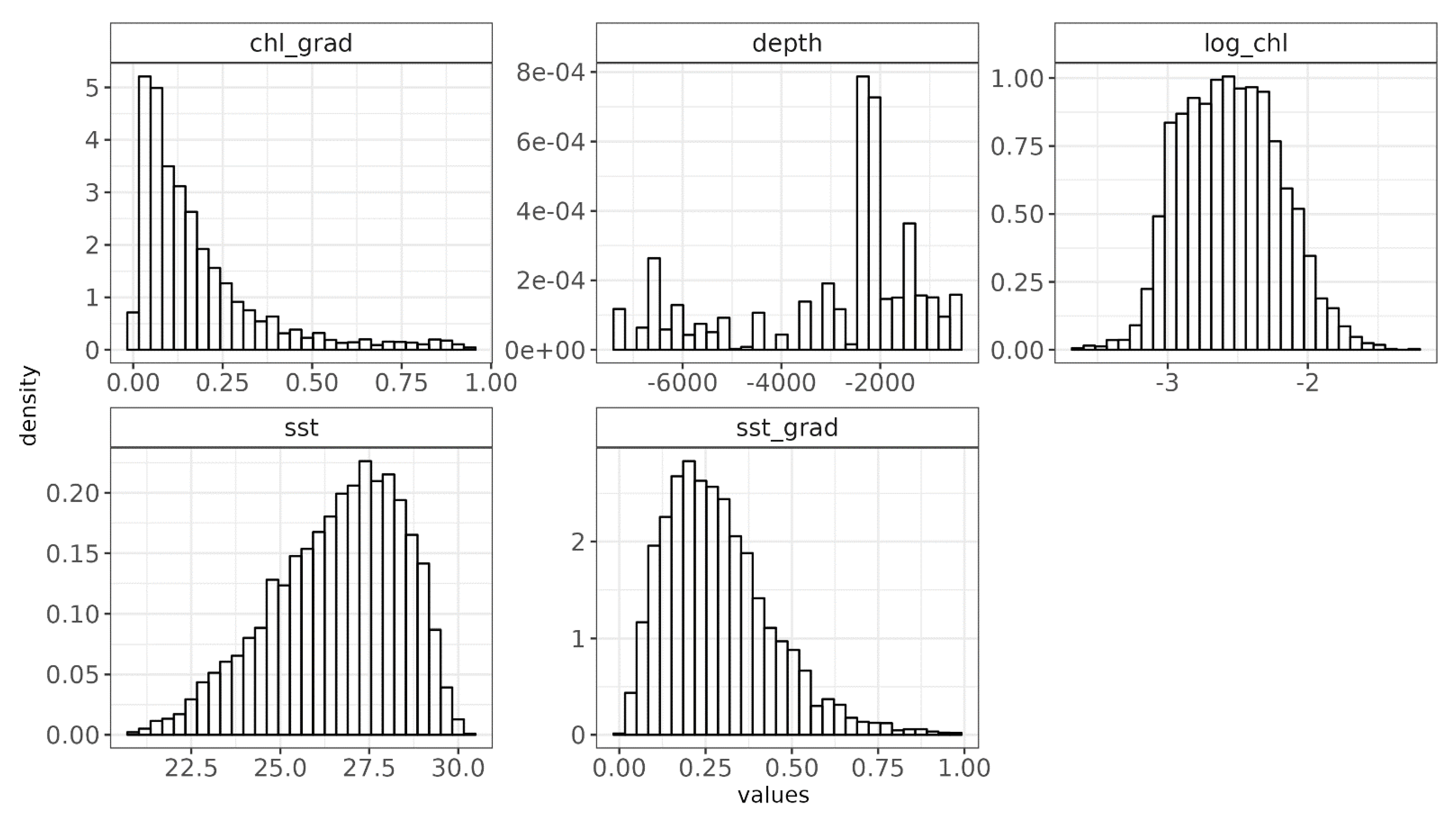
To assess the influence of environmental variables on the distribution of the four tuna species, SST and Chl-a were downloaded from the NOAA repository [33]. Both of these data sources are at a monthly resolution. In addition, to assess the potential influence of fronts regions, frontal gradients for SST and Chl-a were computed for each monthly layer, using the grec R package, version 1.5.0 [34]. These were then normalized by dividing the values by the maximum for the month. The distributions of these environmental variables are shown in Figure 3, respectively. These data made it possible to identify well-defined fronts [35]. Before applying distribution models, the existence and strength of multi-collinearity were assessed. This was completed by computing the variance inflation factor (VIF). There was no indication of the existence of serious multi-collinearity as none of the computed VIF values were more than 5 ( V I F 5 ). Seven GAM models were considered to model the distribution of the four species. Selection among the seven models was based on k-fold cross-validation (where k is repeated 5 times), using root mean squared prediction error (RMSPE) as a performance measure. The seven models considered were:
Model formula M 1 c p u e s s s t M 2 c p u e s s s t + s l o g c h l M 3 c p u e s s s t + s l o g c h l + s d e p t h M 4 c p u e s s s t + s l o g c h l + s d e p t h + s s s t _ g r a d M 5 c p u e s s s t + s l o g c h l + s d e p t h + s s s t _ g r a d + s c h l _ g r a d M 6 c p u e s s s t + s l o g c h l + s d e p t h + s s s t _ g r a d + s c h l _ g r a d + s m o n t h M 7 c p u e s s s t + s l o g c h l + s d e p t h + s s s t _ g r a d + s c h l _ g r a d + s m o n t h + y e a r

2.4. Index of Variable Importance

There are multiple approaches used to compute the relative importance of variables. One such approach applied in the context of species distribution modelling is implemented in the R packages SSDM [36], biomod2 [37]. The approach determines the relative importance of each variable by comparing model predictions under the full model (model with all the variables) to that based on model without the variable of interest. The change in correlation between predictions under the full model to that after removing a predictor indicates how important the removed variable was. The index of importance was computed as shown below:
I r i = 1 m a x c o r P r , P p i , 0
where I r i is the relative index of importance, P r prediction from the best model, P p i is the prediction from the variable i i permuted. To obtain a measure of variability of the relative importance required repeating this process 50 times. All the processing, analysis, visualization, and report generation were performed using multiple packages [38,39,40,41,42,43,44,45,46] in R software [47].

3. Results

3.1. Exploration of the Occurrence

An overview of the distribution of CPUE used in all the distribution modelling is provided in Figures S1–S4 for albacore, bigeye, skipjack, and yellowfin, respectively. The first available data for NASA Aqua was in June 2002, hence the overlay of catch data started over the Tonga EEZ. The figures show monthly and annual distributions of the CPUE of the four species by the longline fishery throughout the year from January to December. The distribution of CPUE shown suggests that most of the fishing effort of the tuna longliners was concentrated in the 15–24° S. Bigeye, skipjack, and yellowfin CPUE shows a central-northernmost distribution, and was caught mainly between 14° S and 22° S. The albacore species thrives in temperate to subtropical regions and exhibits its highest catch rates between the central-southern part of the EEZ. The highest CPUE for all species are observed from 2002–2008 and from 2013–2018 and the lowest CPUE are observed from 2009–2012. In addition, the figure also shows a broad scale seasonality in the CPUE of the four tuna species and an increase in their CPUE especially over the recent period.

3.2. Exploration of Environmental Variables

The spatiotemporal pattern in SST, Chl-a, sea surface temperature gradient, sea surface chlorophyll gradient, and bathymetry data within the EEZ of Tonga are shown in Figures S5–S9, respectively. The distribution of SST is not homogeneous throughout the EEZ of Tonga, with pronounced seasonal variation. The value of the temperature ranges from 18   ° C to 30   ° C . From December to April, the temperature remains between 27   ° C and 30   ° C . From May, it falls significantly to reach its minimum in August, at approximately 18   ° C . SST rises from September until November. The northern part of the EEZ is warmer compared to the central and southern parts. The local relative abundance of the four tuna species increases towards the central part of the EEZ (Figures S1–S4), indicating a preference of tropical tuna species to warmer waters. The distribution of SST shows that, during cooler months (April–October), the fishing operations aggregated in more temperate waters of SST 22   ° C to 30   ° C , where the highest catches occurred. The value of Chl-a concentration was at a range of 0.05 0.1   m g m 3 and was observed to be homogeneous and with no clear spatial and temporal patterns. However, generally there was a higher Chl-a concentration in the central part of the EEZ during summer, from November to January.
Bathymetry in this fishing ground is in the range of approximately 2000 8000 m. The islands of Tonga geographically distributed along the south-west to north-east of the EEZ. Very deep water of more than 5000 m covers the Tonga Trench and to the south-eastern part of the EEZ, with very shallow volcanic sea mounts and a large shelf ≥2000 m deep at north-western part. The sea surface chlorophyll-a gradient ranged from 0 to 0.75 m g m 3 m 1 , with slightly higher gradients occurring in the summer months (November to March) and an increase observed during the cooler months (May to August) in the most recent period of the study. The sea surface temperature gradient exhibited a wide annual variation ranging from 0 to 0.60 °C m 1 with slightly higher values observed in the periods of 2004–2010 and 2014–2017.

3.3. Model Performance

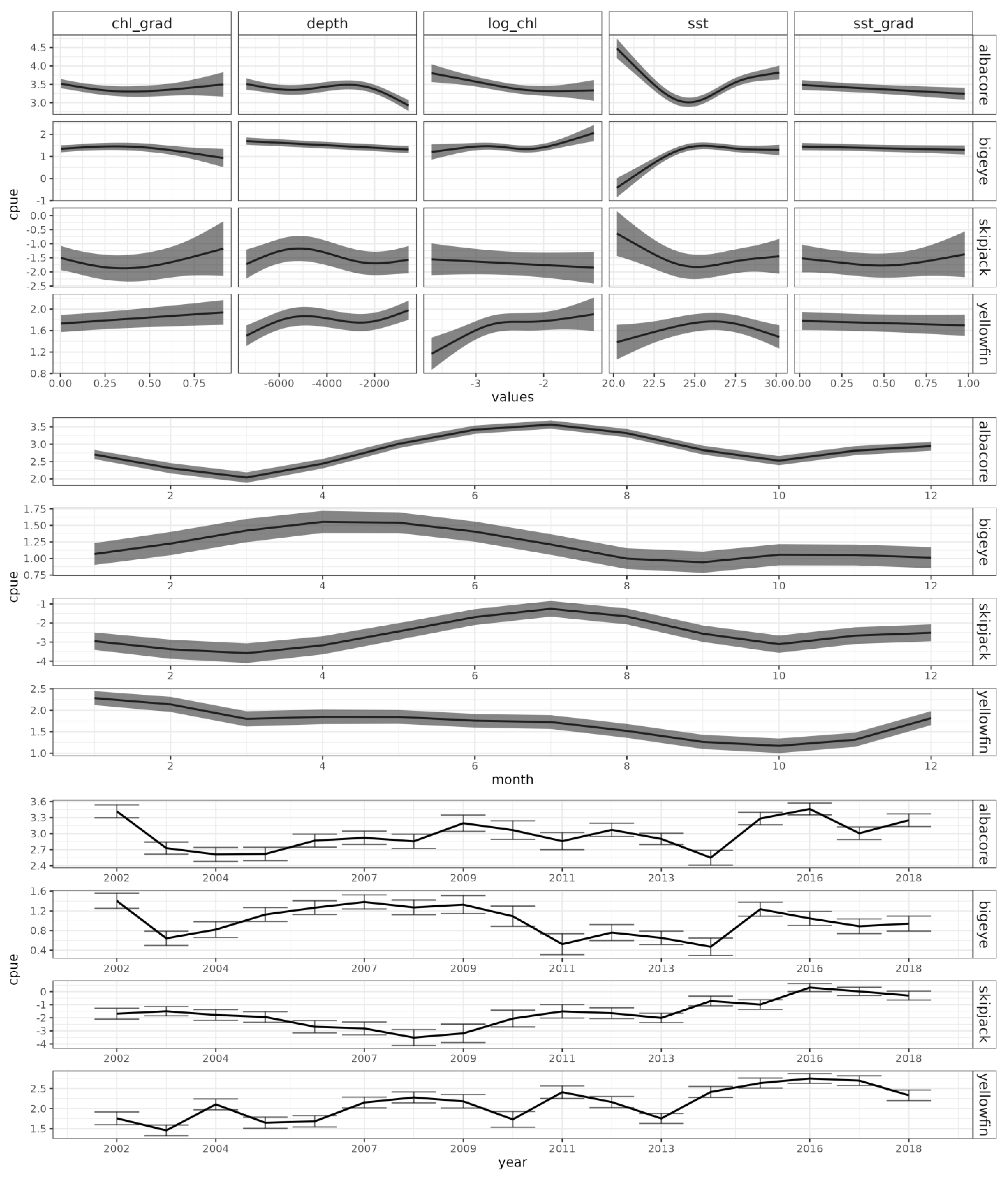
The performance of each of the seven models, from k-fold cross-validation as measured by the RMSPE, is presented in Table 1. Most models with only environmental variables and bathymetry as predictors appear to have comparable performance with noticeable improvement in performance with the addition of catch month and year (e.g., from 11.703 (model 5) to 10.293 (model 7) for albacore). Figure 4 shows the partial effects of predictors on the CPUE of all the four tuna stocks. The partial effects with their partial residuals are presented in Figure S10. For ease of flow, partial effects of all the predictors are presented together. The partial effects of year indicated a gradual increase in CPUE from 2002 to 2018. CPUE appeared to decrease with increases in SST from 20   ° C to about 25   ° C , after which it appeared to increase again. Relatively higher CPUE were also associated with low SST fronts. Albacore appeared to be associated with relatively low chlorophyll water and also a relatively stable chlorophyll front. Within the EEZ of Tonga, albacore appeared to be associated with areas that are deeper with CPUE declining in shallower water <2000 m. Seasonally, higher CPUE were observed around the middle of calendar year. For bigeye tuna, the partial effects of year indicates a gradual increase in CPUE from 2002 to 2007, after which it declined and only started to increase after 2015. The CPUE of bigeye tuna appears to increase with increases in SST up to 25   ° C , after which it remained stable. Relatively higher CPUE were also associated with low SST fronts. Bigeye tuna appear to be associated with relatively high-chlorophyll water and also a relatively stable chlorophyll front. Within the EEZ of Tonga, bigeye appear to be associated with areas that are deeper, with CPUE declining linearly toward shallower water. Seasonally higher CPUE were observed around the start of the calendar year. Plots of predicted values vs. observed values for each species presented in log-scale are shown in Figure S11.
The partial effects of predictors for skipjack tuna are presented in Figure 4. The partial effects of year indicate a gradual decrease in CPUE from 2002 to 2008, after which it gradually increased. The CPUE of skipjack tuna appears to decrease with increases in SST up to 25   ° C , after which it remained relatively stable. The partial effects of chlorophyll indicates that the CPUE of skipjack gradually declined with an increase in l o g   C h l . Although the effects of c h l _ g r a d   are largely flat, they suggests an association of higher CPUE with a low and strong chlorophyll frontal area. A similar pattern appears to characterize the partial effect of s s t _ g r a d on the CPUE of skipjack. Within the EEZ of Tonga, skipjack tuna appear to be associated with areas that are around 5000 m deep with CPUE declining on both sides. Seasonally higher CPUE were observed around July and August.
The partial effects of predictors for yellowfin tuna are presented in Figure 4. The partial effects of year indicates a gradual increase in CPUE from 2002 to 2018 with substantial inter-annual variability. The CPUE of yellowfin tuna appears to increase with increases in SST up to 25   ° C 27   ° C , after which it declined. However, sst frontal ( s s t _ g r a d ) appears to have limited/minor influence on the CPUE of yellowfin tuna. A higher CPUE of yellowfin tuna was associated with water mass characterized by strong chlorophyll fronts ( c h l _ g r a d ). In addition, the CPUE of yellowfin tuna also appears to increase with increases in chlorophyll concentration ( log C h l ). Within the EEZ of Tonga, the CPUE of yellowfin tuna appears to remain stable up to a depth of 5000 m, declining in waters deeper than 5000 m. Seasonally, higher CPUE were observed around July and August.
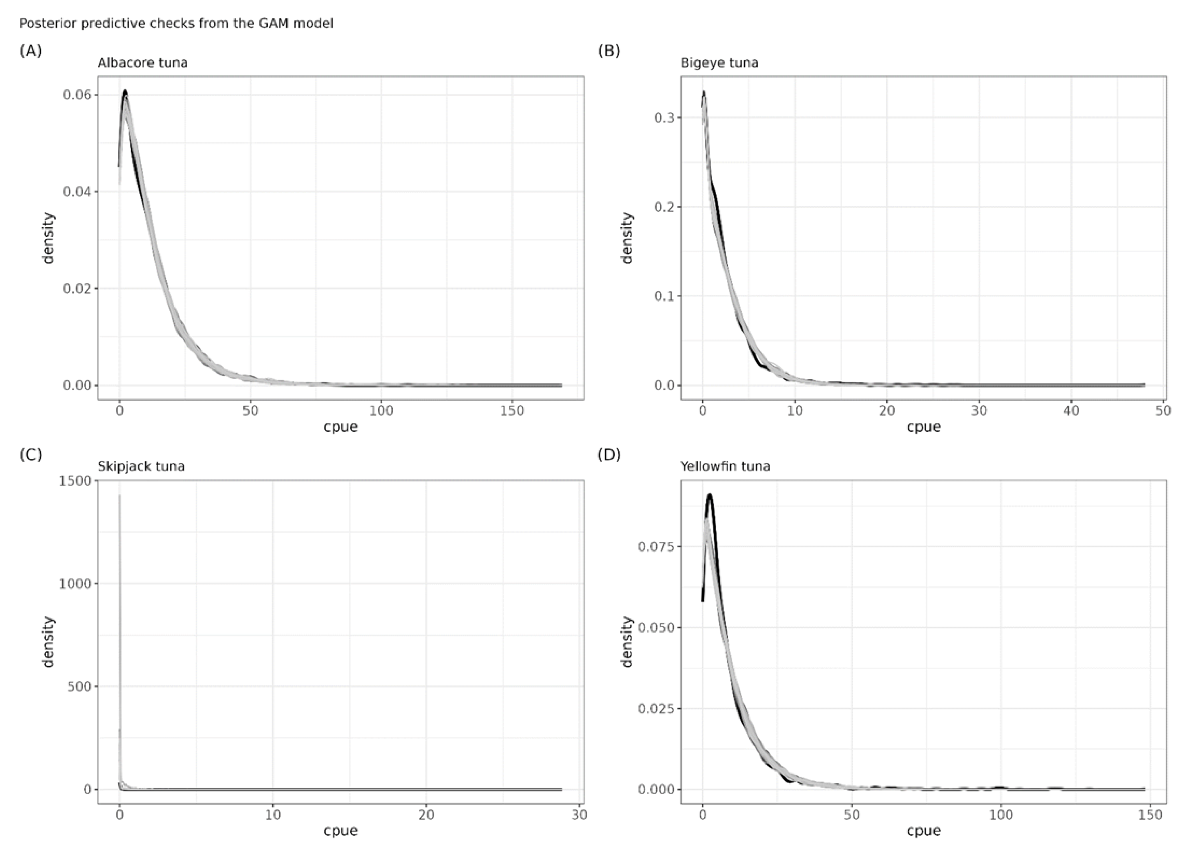
The index of relative importance of the predictors influencing the distribution and abundance of the four tuna populations caught within the EEZ of Tonga is shown in Figure 5. The numerical index of relative importance of predictors for the four tuna species is presented in Table S1. As can be seen in the figure, catch year and catch month were the two most important predictors for all the three species, except for albacore tuna, for which the order reverses. The third most important variable was bottom depth for skipjack and yellowfin tuna and SST for albacore and bigeye tuna. The remaining variables appear to have a minor role. Model diagnostics for the best model were also checked and there was no substantial violation of the assumption of independent and identically distributed variables. Plots of linear predictor vs. deviance residuals and quantile–quantile of residuals are shown in Figure S12 for all species. Figure 6 shows plots of a posterior predictive distribution of the models for the four tuna species. It illustrates that, despite the relatively low deviance explained (Table 2 and Table S2) for all the tuna populations modelled, the model captures the dynamic of the data generation process.
Table 2 presents the cumulative proportion of the deviance explained from the null model to the full model. Table S2 presents smooth effects and Table S3 presents the parametric effects of the best GAM models fitted for each tuna species. As is evident from Table 2, the full models (models including all terms) demonstrate the highest cumulative deviance explained across all species, with albacore having the highest value at 27.622, followed by skipjack and yellowfin, while bigeye has the lowest value at 12.183. Also, it can be seen (Table S2) that all of the smooth terms were significant for albacore (with p-value < 0.05). For bigeye tuna, sst_grad was not statistically significant, whereas the remaining terms had a significant effect. The effects of both frontal terms (sst_grad and chl_grad) and chlorophyll were not significant for skipjack tuna with SST, bottom depth, and month having statistically significant effects. For yellowfin tuna, all the terms, except for sst_grad, had a significant effect on its spatiotemporal pattern.

3.4. Standardized Index of Abundance

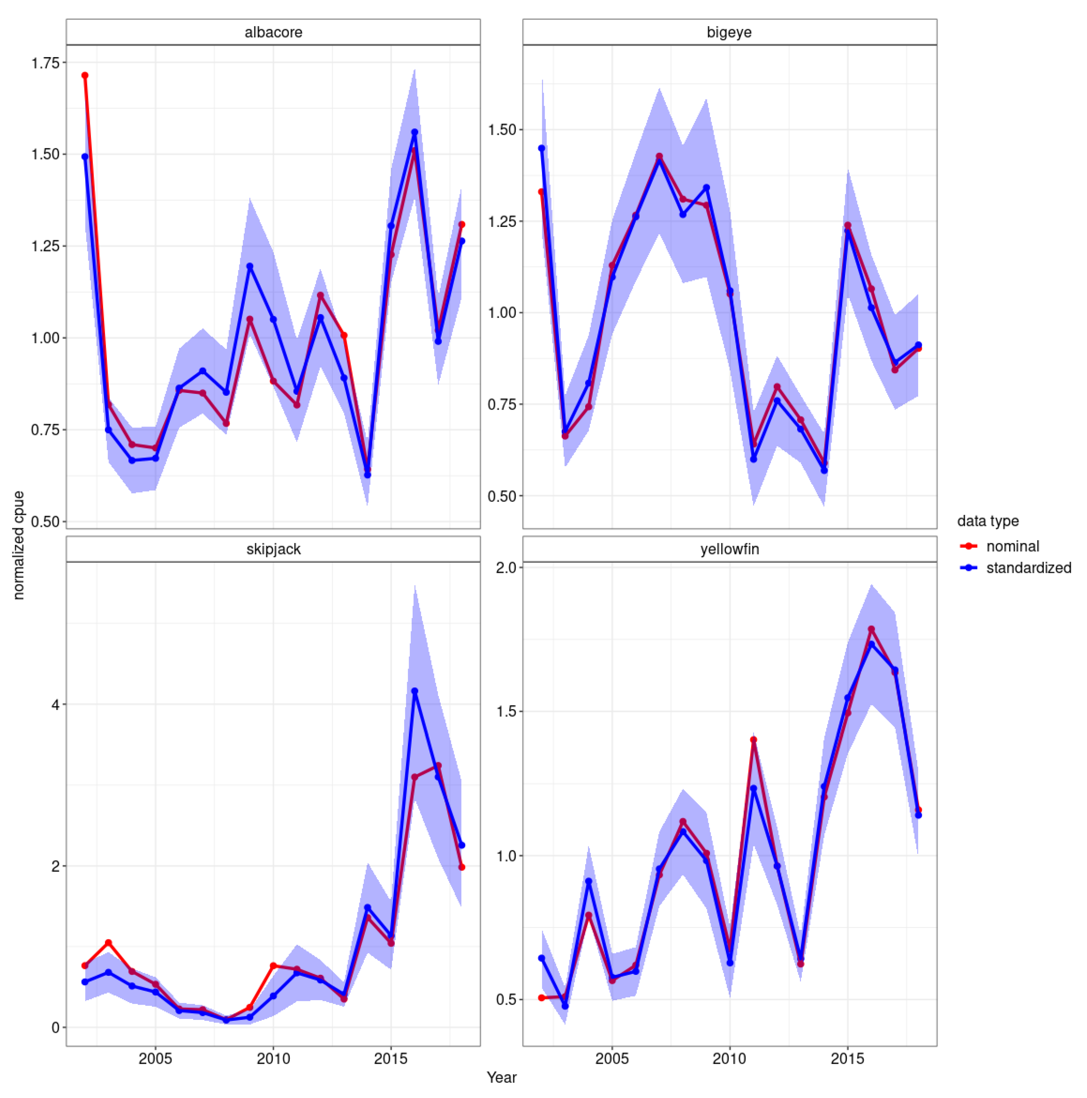
The standardized index of abundance, based on the best GAM model, is presented in Figure 7. For comparison, both the standardized and nominal index of abundance were normalized, I n = I / I ¯ . The trends for both albacore and bigeye tuna are characterized by inter-annual variability with no long-term trend over the period considered. Skipjack and yellowfin tuna appear to show an overall increase in abundance over the period 2002–2018.
.

3.5. Map of Predicted Suitable Habitat

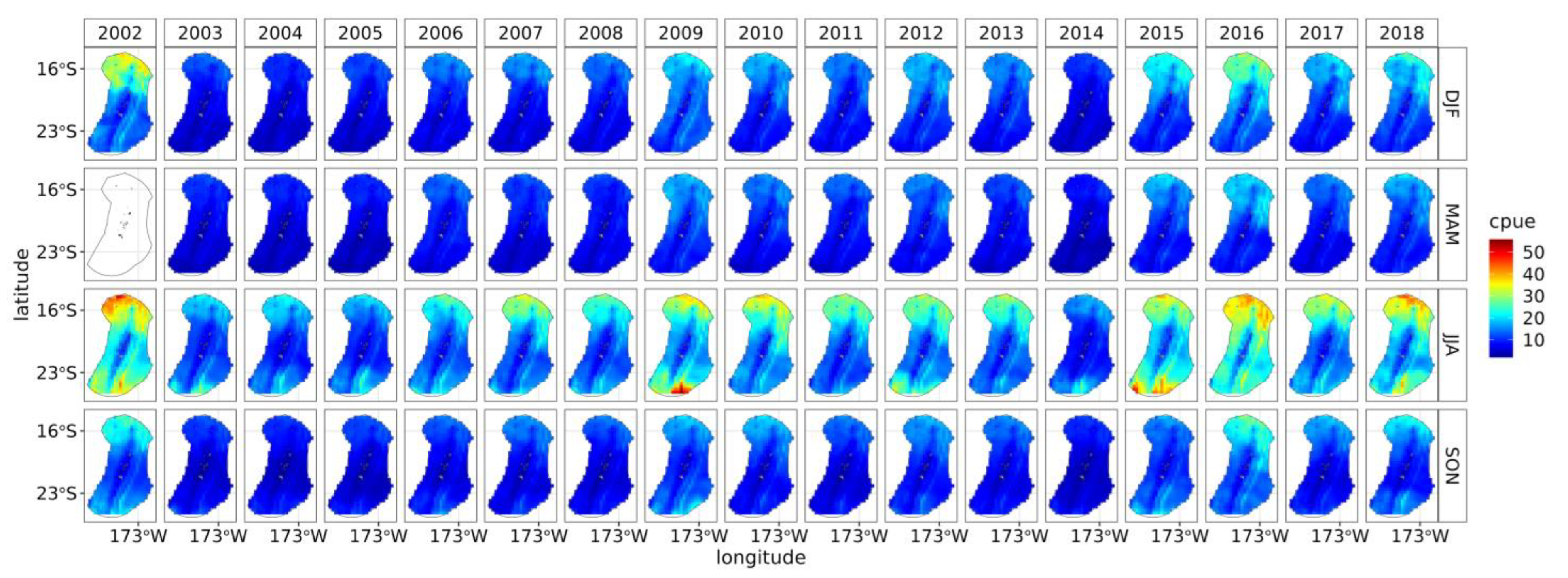
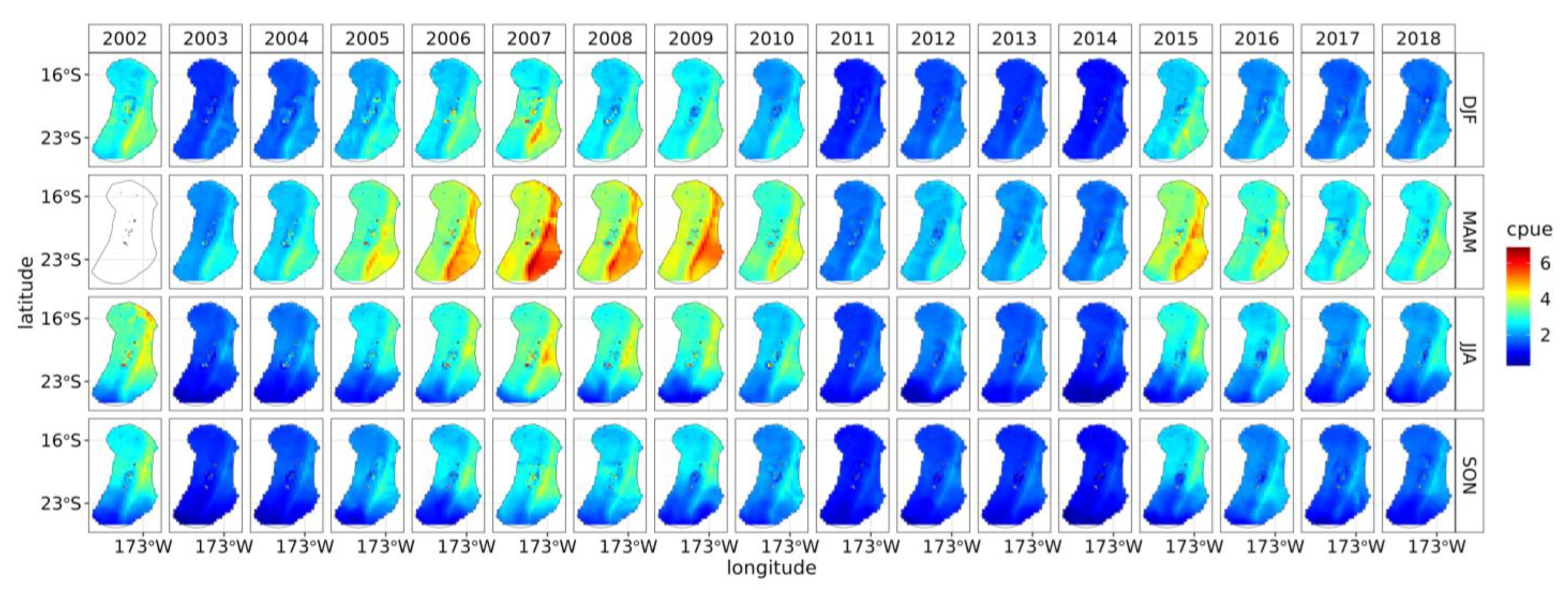
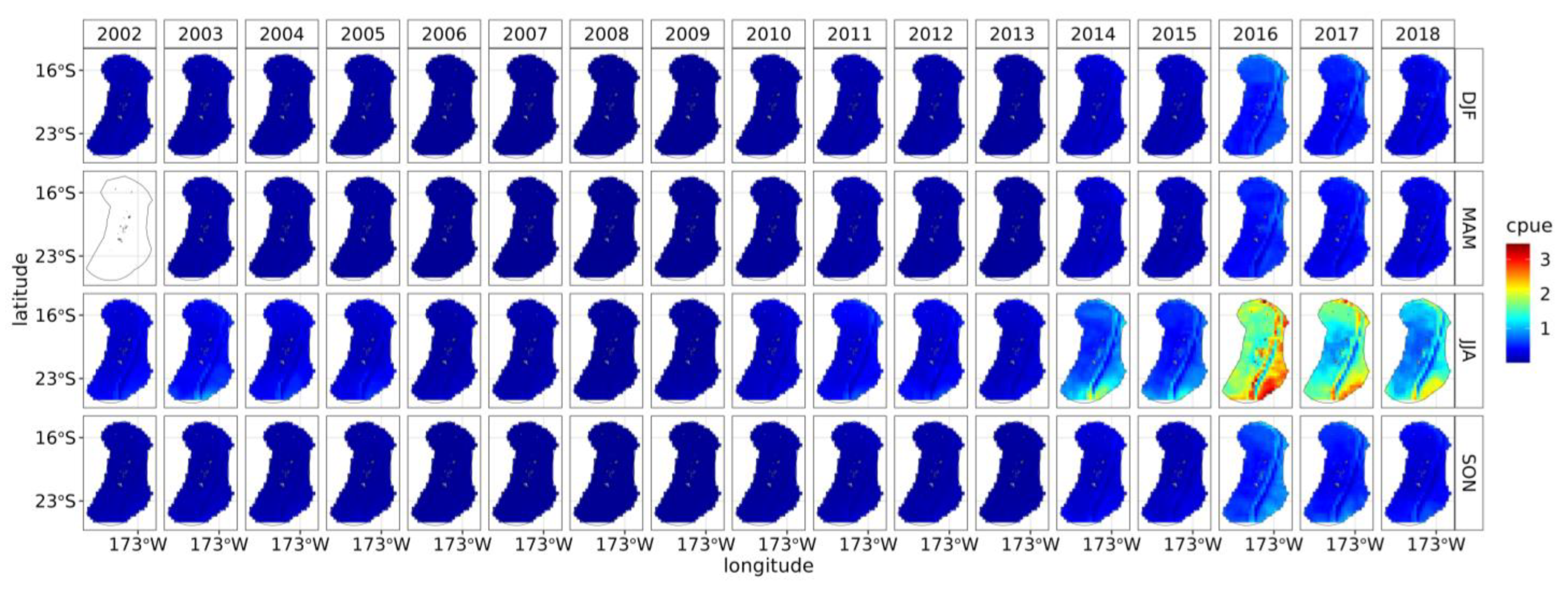
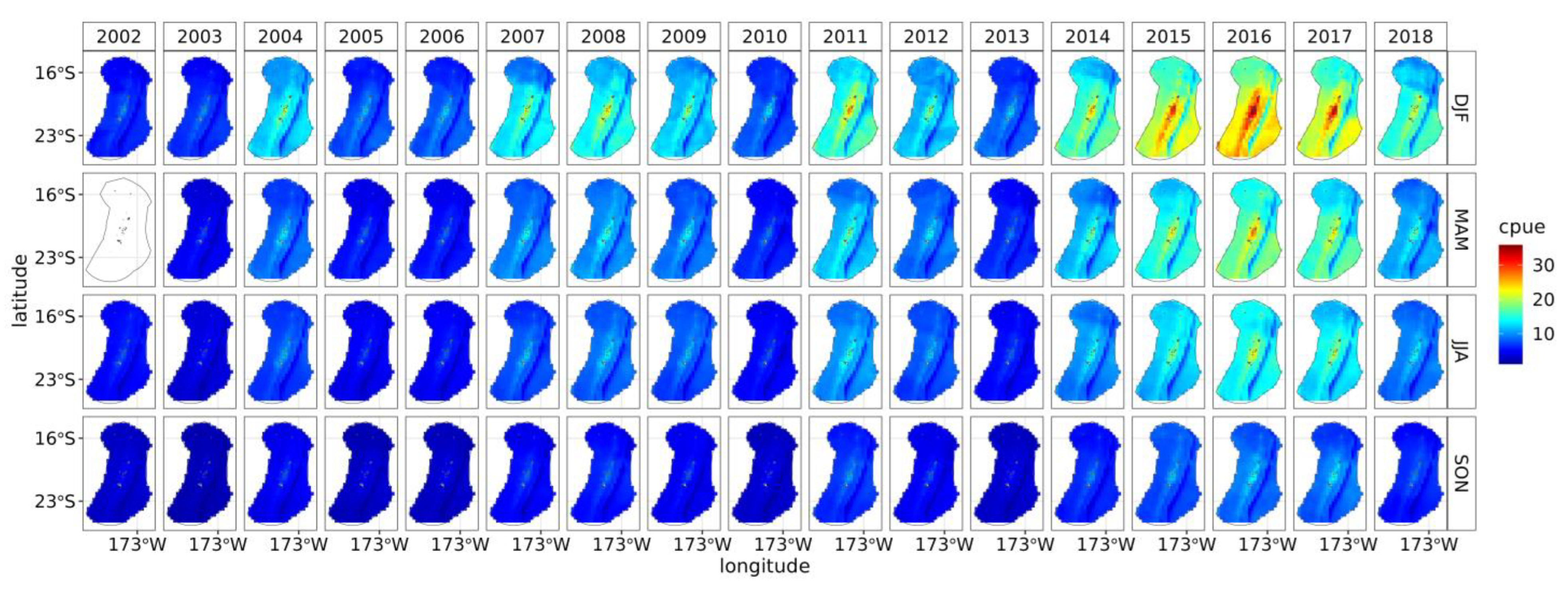
Maps of predicted suitable habitat for albacore, bigeye, skipjack, and yellowfin are shown in Figure 8, Figure 9, Figure 10 and Figure 11. They are arranged quarterly to illustrate how their abundance changes with season. Albacore tuna appeared to be characterized by seasonal variability in CPUE where they become more abundant during the months of July to August, with regions in the northern and southern parts of the EEZ characterized by relatively higher abundance (Figure 8). Conversely, as shown in Figure 9, bigeye tuna appeared to be more abundant during the first half of the year (January–June) and in regions in the southern and eastern part of the EEZ. Although skipjack increased in abundance after 2013 (Figure 10), they appeared to be characterized by the same seasonal cycle as albacore tuna and peak in abundance around July to August, but are associated with the same regions as bigeye tuna. Yellowfin tuna has also been increasing in abundance since about 2010; although characterized by inter-annual variability, they appear to be in higher abundance from December to July and mostly around the island chain (Figure 11).

4. Discussion

Our purpose in modeling albacore, bigeye, yellowfin, and skipjack distribution in the EEZ of Tonga was to link tuna CPUE to environmental, physical, and temporal factors and subsequently to generate predictive habitat suitability maps and standardized indices of abundance, which could be useful for national planning and policy development for conservation and sustainable management of the species. The environmental variables included in this study were SST, Chl-a, sst grad, chl_grad and bottom depth (as physical predictors). Other variables (e.g., salinity levels, mixed layer depth, sea surface height, ocean currents, dissolved oxygen, and others) have been employed in previous studies as predictors when modeling the suitability of tuna habitats [49,50,51,52,53,54]. Studies indicate that these surface and subsurface layers of oceanic environments also influence the distribution and presence of tuna in the water column. The movement of ocean surface waters, including converging and diverging flows, is linked to fluctuations in sea surface height. Tuna utilize these variations as signals to identify areas where food is plentiful. [49]. The movement of ocean currents has an effect on the mobility of phytoplankton and small pelagic fish, thus shaping the dispersion of marine organisms at higher trophic levels [50]. The distribution and presence of tuna in the ocean environment are also influenced by dissolved oxygen levels [51] and salinity [52,53]. However, when accessible, these investigations are constrained either to a single species or to relatively small regions [7]. Furthermore, when these variables are integrated with sea surface temperature and chlorophyll concentration to model habitat suitability, research has indicated that SST and Chl-a concentration are the predominant factors among them [3,10,19,55,56,57]. Our study also included extensive tuna longline datasets with spatiotemporal coverages, where the information was used to model tuna habitat preferences and distribution as a number of studies have shown [58,59,60]. It may be premature to draw strong inferences regarding environmental effects on tuna distribution and abundance, even so, our results indicated that temporal variables, e.g., inter-annual variability and seasonality are influential. Bottom depth served as surrogate for environmental conditions not captured by SST, Chl-a, and the two frontal indices (sst_grad, and chl_grad). This played an important role following year and month for all the tuna species considered except for albacore tuna. SST was the most important variable following year, month, and bottom depth for all the tuna species considered in this study. GAM analysis, modeling the CPUE of tuna species, revealed that catch year and catch month had biggest effect (Figure 4) on the fisheries success.
Although no scientific studies have been conducted on tuna habitat preferences in Tonga, areas with relatively high CPUE of tuna species could be attributed to oceanographic conditions associated the bathypelagic features within its EEZ. As previously stated, this central part of the EEZ partly envelops the Tonga Ridge, Tofua Arce Volcanic Front, the northern end of the Tonga Kermadec Arc, the westward region of the Lau Basin and the parallel north to south chains of volcanic seamounts along the Tonga Ridge. These oceanic features may influence environmental conditions, such as surface water temperature, nutrient, salt content, and mixed layer depth, which are habitats for pelagic species such as tuna. This may also be the reason for the persistent presence of the four tuna species throughout the year although the EEZ of Tonga is part of the WCPO and is generally characterized as oligotrophic [61], due to deep vertical mixing of water masses. Studies have demonstrated a strong correlation between tuna and shallow waters, particularly continental shelves and seamounts [62,63]. These locations are widely recognized as prime habitats for large offshore fishes, primarily because of the substantial foraging advantages they offer [62] and possibly for reproductive and navigational benefits [64,65,66].
The temporal pattern in the standardized indices of abundance (Figure 7) and the partial effects plots suggested that during the time period of this study (2002–2018), some of the stocks of the tuna population within the EEZ of Tonga experienced a gradual increase, whereas for other species it was mostly characterized by inter-annual variability. Some of the important regulatory changes and environmental dynamics within the time period of this study that could potentially be driving the trend in the CPUE of the four tuna populations within the EEZ include: (i) a fishing moratorium (2004–2011) on foreign fishing fleets [1], as part of the Tonga’s long-term plan to expand its tuna fisheries, and (ii) the impact of El Niño Southern Oscillation (ENSO) events (such as those of 1997/98, 2003/04, 2009/10) known to affect tuna catchability through the spatial shift of tuna’s preferred habitat away from normal fishing grounds in the Western Pacific [67,68]. Strong seasonality was observed in the distribution and abundance of tuna populations. This could be attributed to seasonal variability, which is known to influence the migration patterns and habitats of tuna in the WCPO [5,13]. Whilst Zainuddin et al., (2008) reported increased tuna abundance in cooler waters (April-September) in the Western North Pacific Ocean, Arrizabalaga et al. (2015) [20] reported higher abundance in warm waters due to tuna temperature preference for spawning.
Bathymetry also plays a role (Figure 5) in the central area of the EEZ of depths ranged between 2000   m   a n d   3000   m (Figure S9), where the highest tuna capture occurred. As stated above, this is an area that partly envelops water of various depths due to its geographically topographic features. The eastern part of the EEZ covers the famous Tonga Trench, which runs south–north with depths of 5000   m or greater.
Our CPUE distributions (Figures S1–S4) show this area to have very low tuna encounters as compared to the central part. We attributed this habitat suitability distribution to two main reasons: (i) the productive waters in the deep areas are scattered over large vertical waters, whereas in smaller vertical waters, productive waters are compressed making them easy and quick to access for tuna, hence a higher tuna presence; (ii) since bathymetry is linked to both fleet operations and fish habitat; hence, it can act as a crude proxy for distance from ports. The distance from the main ports in Nuku’alofa (the capital of Tonga) to the high tuna occurrence areas (central areas of the EEZ) is in the range of 50 to 100 km, whereas the distance to the deepest areas is in the range of 150 to 400 km. Therefore, it could be that fishing vessels preferred the central area due to its shorter distance from ports, hence cutting back on operational costs.
The preferred ranges of the environmental factors, SST and Chl-a, are shown in Figure 4, but were found to be least important in modelling distribution, as measured by variable importance (values 0.1 , Figure 5); much less important than spatial-temporal factors and bottom depth. Therefore, we tend to consider their influence over the tuna occurrence in the EEZ of Tonga to be limited (at least in the context of the present modelling framework). A study by Lan et al. (2017) [19] in the Tropical Pacific Ocean, suggests that areas with a higher SST and a Chl-a concentration of approximately 0.05–0.25 m g m 3 yield higher catch rates of yellowfin tuna. Setiawati et al. (2015) [10] indicated bigeye tuna habitat ranges for SST and Chl-a are 24.8 to 28.7 °C and 0.05 to 0.17 m g m 3 , respectively. The results indicated by Zainuddin et al. (2006) that the distribution pattern of potential fishing zones for skipjack during the southeast monsoon were well-characterized by SST, ranging from 28.5 °C to 30.5 °C and with Chl-a ranging from 0.10 to 0.20 m g m 3 [55]. In the Western Pacific Ocean, Zainuddin et al. (2008) report that the highest CPUE of albacore corresponded with areas of SST at 18.5–21.5 °C and Chl-a of 0.2–0.4 m g m 3 [69]. In addition, studies have shown that areas with low catch encounters are found in the offshore waters due to the low Chl-a concentration present in these areas [69,70]. Chl-a presence is an indicator of areas where small pelagic fishes concentrated for feeding [71]. Hence, an adequate level of Chl-a concentration is required to enhance food availability and increase fish presence in the area. According to Atkinson et al. (2001) [72], Chl-a concentration of at least 0.2   m g m 3 is required (as compared to the Chl-a concentration in the EEZ of Tonga 0.03 0.1   m g m 3 ) to provide adequate levels of food to support a viable commerical fishery. Our results show that the highest Chl-a concentration in the archipelago waters of Tonga to be 0.1   m g m 3 , which is only half of that reported ( 0.2   m g m 3 ). Furthermore, there is no direct input of nutrient from land and coastal upwellings [61] to enhance primary productivity [73,74].
The spatiotemporal pattern in SST and Chl-a data (Figure S5 and Figure S6, respectively) show their monthly variability compared to maps of predicted suitable habitat for albacore (Figure 8), bigeye (Figure 9), skipjack (Figure 10), and for yellowfin (Figure 11). It was observed, as stated earlier, that the largest captures of the four tuna species are distributed in the central waters, 15 °   S 24 °   S , of the EEZ with temperatures above 22   ° C and Chl-a concentration 0.001   m g m 3 . Our results show that albacore has the highest CPUE, followed by bigeye and yellowfin, and skipjack has the lowest as indicated by CPUE distributions (Figures S1–S4). The study by Arrizabalaga et al. (2015) [20] on global tuna catch found that albacore has the highest CPUE and is mostly caught between the latitudes of 20 °   S   a n d   40 °   N , relatively high bigeye CPUE has been observed between 0 °   a n d   40 ° of each hemisphere, and yellowfin are found around the equator, while skipjack’s highest CPUE are observed around 0 ° 20 ° of each hemisphere. The study by Hu et al. (2018) [75] found that bigeye tuna are caught more (more so than yellowfin, albacore, and skipjack) in equatorial waters farther from the coast and where the hypoxic layer is deeper. There was also indication of seasonal variation in their distributions, possibly corresponding to seasonal displacement of water temperature along low–high latitudes [76]. Our results show they influence but do not seem to be the main determinants of the distribution and abundance of the tuna species in Tongan waters when compared, for example, to temporal measures like the variables month and year (Figure 5).

5. Conclusions

The study integrated catch data for four tuna species in Tonga’s EEZ with satellite-derived environmental data and employed distribution modeling and GAM analyses, revealing that high tuna catches align closely with predicted habitat maps from 2002 to 2018. The partial effect plots of our GAMs confirmed the non-linear relationships between the variables analyzed and tuna occurrence. Among the variables considered, SST exhibited the highest importance, followed by year, month, and bottom depth for all the tuna species in this study. The results of our study also suggest that the stocks of tuna populations within Tonga’s EEZ showed a gradual increase for some species while others exhibited inter-annual variability. The key factors driving the CPUE trends for the four tuna populations could be attributed to a fishing moratorium on foreign fleets and the influence of El Niño-Southern Oscillation events altering the preferred habitat of tuna. Regarding spatial distribution, both the CPUE distribution and the predicted suitable tuna habitats in the study region indicate a preference for the tuna species to be concentrated in the central part of the EEZ, aligning with historically productive tuna fishing areas. The study revealed a seasonal peak in tuna occurrence between May and September, contrasting with lower occurrence rates from October to April, underscoring the consistent significance of spatiotemporal variables in shaping the habitat patterns of tuna and highlighting specific times and locations of abundance for these species. Overall, our model results predict the spatiotemporal pattern of the four tuna habitats in good agreement with our simple prediction maps and observation occurrence data. Future research needs to be conducted in the area in order to further examine the links and interactions between tuna habitats and other environmental and oceanographic factors not included in this study.

Supplementary Materials

The following supporting information can be downloaded at: https://www.mdpi.com/article/10.3390/d15101091/s1, Table S1. Summary of numerical index of relative importance of predictors for the four tuna species in the EEZ, of Tonga. Table S2. Model summary for the best GAM model for the four species. Smooth effects: estimated degrees of freedom (edf), degrees of freedom (df), F-statistics, and p-values and deviance explained are presented. Table S3. Model summary for the best GAM model for the four species. Parametric effects: estimate, standard error, F-statistics and p-values are presented. Figure S1. Spatiotemporal pattern in the distribution of albacore tuna within the EEZ of Tonga, l o n g i t u d e   14.5 °   S 20.22 °   S , longitude 171.31 °   W 179.10 °   W . Data aggregated to coarser resolution of 0.3 degree (~5 NM). Figure S2. Spatiotemporal pattern in the distribution of bigeye tuna in the EEZ of Tonga, l o n g i t u d e   14.5 °   S 20.22 °   S , longitude 171.31 °   W 179.10 °   W . Data aggregated to coarser resolution of 0.3 degree (~5 NM). Figure S3. Spatiotemporal pattern in the distribution of skipjack tuna in the EEZ of Tonga, l o n g i t u d e   14.5 °   S 20.22 °   S , longitude 171.31 °   W 179.10 °   W . Data aggregated to coarser resolution of 0.3 degree (~5 NM). Figure S4. Spatiotemporal pattern in the distribution of yellowfin tuna in the EEZ of Tonga, l o n g i t u d e   14.5 °   S 20.22 °   S , longitude 171.31 °   W 179.10 °   W . Data aggregated to coarser resolution of 0.3 degree (~5 NM). Figure S5. Annual and monthly variability of sea surface temperature for the EEZ of Tonga, l o n g i t u d e   14.5 °   S 20.22 °   S , longitude 171.31 °   W 179.10 °   W . Data aggregated to coarser resolution of 0.3 degree (~5 NM). Figure S6. Annual and monthly variability of sea surface chlorophyll for the EEZ of Tonga, l o n g i t u d e   14.5 °   S 20.22 °   S , longitude 171.31 °   W 179.10 °   W . Figure S7. Annual and monthly variability of sea surface chlorophyll gradient for the EEZ of Tonga, l o n g i t u d e   14.5 °   S 20.22 °   S , longitude 171.31 °   W 179.10 °   W . Figure S8. Annual and monthly variability of sea surface temperature gradient for the EEZ of Tonga, l o n g i t u d e   14.5 °   S 20.22 °   S , longitude 171.31 °   W 179.10 °   W . Figure S9. Bathymetry for the EEZ of Tonga, l o n g i t u d e   14.5 °   S 20.22 °   S , longitude 171.31 °   W 179.10 °   W . Figure S10. The partial effects with partial residuals for covariates chl_grad, depth, Chl-a, SST, sst_grad, month and year for (a) albacore, (b) bigeye, (c) skipjack and (d) yellowfin, respectively, within the EEZ of Tonga, longitude 171.31 °   W 179.10 °   W . Figure S11. Model diagnostic plots of predicted values vs. observed values for each species presented in log-scale for visual purpose. Figure S12. Model diagnostics, plot of linear predictors vs. deviance residuals and quantile–quantile plots of theoretical values vs. deviance residuals for albacore (panels A and B), bigeye (panels C and D), skipjack (panels E and F) and yellowfin (panels G and H) in the EEZ of Tonga, l o n g i t u d e   14.5 °   S 20.22 °   S , longitude 171.31 °   W 179.10 °   W .

Author Contributions

Data curation, conceptualization, methodology, software, validation, and formal analysis were conducted by D.Y. and S.V. S.V. and D.Y. wrote the draft manuscript with input from S.K. All authors contributed to the critical revision and approval of the final manuscript. S.K. supervised the project. All authors have read and agreed to the published version of the manuscript.

Funding

The Pacific European Marine Program (PEUMP) grant number F3288 funded this research, and the APC was also funded by PEUMP.

Institutional Review Board Statement

Not applicable.

Data Availability Statement

All species data and extracted predictor variables are available in: VAIHOLA, SIOSAIA (2023), Tonga tuna, Dryad, Dataset: https://datadryad.org/stash/share/Bkhr8-Suq6P0M3Q8MZ7XYymkqiy4kl2DQwfk39c5MhQ (accessed on 12 September 2023).

Acknowledgments

The authors would like to thank the Pacific European Marine Program for financially supporting this study and the Tonga Ministry of Agriculture, Forestry and Fisheries and the SPC for providing the fishery datasets from the Tonga longline fishery industry. Also, the authors acknowledge NOAA of the USA for the environmental and bathymetry remotely sensed datasets and the R community.

Conflicts of Interest

The authors declare no conflict of interest.

References

  1. MAFF; FFA. Tonga Tuna Fishery Framework 2018–2022; Fishery Forum Agency; Ministry of Agriculture, Forestry, Fisheries: Nuku’alofa, Tonga, 2018. [Google Scholar]
  2. Brouwer, S.; Pilling, G.; Hampton, J.; Williams, P.; McKechnie, S.; Tremblay-Boyer, L. The Western and Central Pacific Tuna Fishery: 2017 Overview and Status of Stocks; Tuna Fisheries Assessment Report; Pacific Community: Noumea, New Caledonia, 2018; Volume 18. [Google Scholar]
  3. Lan, K.-W.; Shimada, T.; Lee, M.A.; Su, N.J.; Chang, Y. Using remote-sensing environmental and fishery data to map potential yellowfin tuna habitats in the tropical pacific ocean. Remote Sens. 2017, 9, 444. [Google Scholar] [CrossRef]
  4. Yen, K.W.; Lu, H.J.; Chang, Y.; Lee, M.A. Using remote-sensing data to detect habitat suitability for yellowfin tuna in the western and central pacific ocean. Int. J. Remote Sens. 2012, 33, 7507–7522. [Google Scholar] [CrossRef]
  5. Mainuddin, M.; Saiton, K.; Saiton, S. Albacore fishing ground in relation to oceanographic conditions in the western north pacific ocean using remotely sensed satellite data. Fish. Oceanogr. 2008, 17, 61–73. [Google Scholar] [CrossRef]
  6. Solanki, H.; Prakash, P.; Dwivedi, R.; Nayak, S.; Kulkarni, A.; Somvamshi, V. Synergistic application of oceanographic variables from multi-satellite sensors for forecasting potential fishing zones: Methodology and validation results. Int. J. Remote Sens. 2010, 31, 775–789. [Google Scholar] [CrossRef]
  7. Dell, J.; Wilcox, C.; Hobday, A.J. Estimation of yellowfin tuna (Thunnus albacares) habitat in waters adjacent to australia’s east coast: Making the most of commercial catch data. Fish. Oceanogr. 2011, 20, 383–396. [Google Scholar] [CrossRef]
  8. Harrison, D.P.; Hinton, M.G.; Kohin, S.; Armstrong, E.M.; Snyder, S.; O’Brien, F.; Kiefer, D.K. The pelagic habitat analysis module for ecosystem-based fisheries science and management. Fish. Oceanogr. 2017, 26, 316–335. [Google Scholar] [CrossRef]
  9. Hidayat, R.; Zainuddin, M.; Putri, A.R.S. Skipjack tuna (Katsuwonus pelamis) catches in relation to chlorophyll-a front in bone gulf during the southeast monsoon. Aquac. Aquar. Conserv. Legis. 2019, 12, 209–218. [Google Scholar]
  10. Setiawati, M.D.; Sambah, A.B.; Miura, F.; Tanaka, T.; As-syakur, A.R. Characterization of bigeye tuna habitat in the Southern Waters off Java-Bali using remote sensing data. Adv. Space Res. 2015, 55, 732–746. [Google Scholar] [CrossRef]
  11. Wang, W.; Zhou, C.; Shao, Q.; Mulla, D. Remote sensing of sea surface temperature and chlorophyll-a: Implications for squid fisheries in the north-west pacific ocean. Int. J. Remote Sens. 2010, 31, 4515–4530. [Google Scholar] [CrossRef]
  12. Wang, Y.; Liu, J.; Liu, H.; Lin, P.; Yuan, Y.; Chai, F. Seasonal and interannual variability in the sea surface temperature front in the eastern pacific ocean. J. Geophys. Res. Ocean. 2021, 126, e2020JC016356. [Google Scholar] [CrossRef]
  13. Wiryawan, B.; Loneragan, N.; Mardhiah, U.; Kleinertz, S.; Wahyuningrum, P.I.; Pingkan, J. Catch per unit effort dynamic of Yellowfin Tuna related to sea surface temperature and chlorophyll in southern Indonesia. Fishes 2020, 5, 28. [Google Scholar] [CrossRef]
  14. Zainuddin, M. Skipjack tuna in relation to sea surface temperature and chlorophyll-a concentration of Bone Bay using remotely sensed satellite data. J. Ilmu Dan Teknol. Kelaut. Trop. 2011, 3. [Google Scholar] [CrossRef]
  15. Zainuddin, M.; Nelwan, A.; Farhum, S.A.; Hajar, M.A.I.; Kurnia, M. Characterizing potential fishing zone of skipjack tuna during the southeast monsoon in the Bone Bay-Flores Sea using remotely sensed oceanographic data. Int. J. Geosci. 2013, 4, 259–266. [Google Scholar] [CrossRef]
  16. Sambah, A.B.; Muamanah, A.; Harlyan, L.I.; Lelono, T.D.; Iranawati, F.; Sartimbul, A. Sea surface temperature and chlorophyll-a distribution from Himawari satellite and its relation to yellowfin tuna in the Indian Ocean. Aquac. Aquar. Conserv. Legis. 2021, 14, 897–909. [Google Scholar]
  17. Huot, Y.; Morel, A.; Twardowski, M.S.; Stramski, D.; Reynolds, R.A. Particle optical backscattering along a chlorophyll gradient in the upper layer of the eastern South Pacific Ocean. Biogeosciences 2008, 5, 495–507. [Google Scholar] [CrossRef]
  18. Stoner, A.W. Effects of environmental variables on fish feeding ecology: Implications for the performance of baited fishing gear and stock assessment. J. Fish Biol. 2004, 65, 1445–1471. [Google Scholar] [CrossRef]
  19. Mugo, R.; Saitoh, S.I.; Nihira, A.; Kuroyama, T. Habitat characteristics of skipjack tuna (Katsuwonus pelamis) in the western North Pacific: A remote sensing perspective. Fish. Oceanogr. 2010, 19, 382–396. [Google Scholar] [CrossRef]
  20. Arrizabalaga, H.; Dufour, F.; Kell, L.; Merino, G.; Ibaibarriaga, L.; Chust, G. Global habitat preferences of commercially valuable tuna. Deep Sea Res. Part II Top. Stud. Oceanogr. 2015, 113, 102–112. [Google Scholar] [CrossRef]
  21. Putri, A.R.S.; Zainuddin, M.; Musbir, M.; Mustapha, M.A.; Hidayat, R.; Putri, R.S. May. Impact of increasing sea surface temperature on skipjack tuna habitat in the Flores Sea, Indonesia. IOP Conf. Ser. Earth Environ. Sci. 2021, 763, 012012. [Google Scholar] [CrossRef]
  22. Karnauskas, K.B.; Seager, R.; Kaplan, A.; Kushnir, Y.; Cane, M.A. Observed strengthening of the zonal sea surface temperature gradient across the equatorial Pacific Ocean. J. Clim. 2009, 22, 4316–4321. [Google Scholar] [CrossRef]
  23. Seager, R.; Cane, M.; Henderson, N.; Lee, D.E.; Abernathey, R.; Zhang, H. Strengthening tropical Pacific zonal sea surface temperature gradient consistent with rising greenhouse gases. Nat. Clim. Chang. 2019, 9, 517–522. [Google Scholar] [CrossRef]
  24. Nishida, T.; Mohri, M.; Itoh, K.; Nakagome, J. Study of bathymetry effects on the nominal hooking rates of yellowfin tuna (Thunnus albacares) and bigeye tuna (Thunnus obesus) exploited by the japanese tuna longline fisheries in the indian ocean. IOTC Proc. 2001, 4, 191–206. [Google Scholar]
  25. Schick, R.S.; Goldstein, J.; Lutcavage, M.E. Bluefin tuna (Thunnus thynnus) distribution in relation to sea surface temperature fronts in the Gulf of Maine (1994–1996). Fish. Oceanogr. 2004, 13, 225–238. [Google Scholar] [CrossRef]
  26. Zainuddin, M.; Farhum, A.; Safruddin, S.; Selamat, M.B.; Sudirman, S.; Nurdin, N.; Syamsuddin, M.; Ridwan, M.; Saitoh, S.I. Detection of pelagic habitat hotspots for skipjack tuna in the Gulf of Bone-Flores Sea, southwestern Coral Triangle tuna, Indonesia. PLoS ONE 2017, 12, e0185601. [Google Scholar] [CrossRef] [PubMed]
  27. Druon, J.N.; Fromentin, J.M.; Aulanier, F.; Heikkonen, J. Potential feeding and spawning habitats of Atlantic bluefin tuna in the Mediterranean Sea. Mar. Ecol. Prog. Ser. 2011, 439, 223–240. [Google Scholar] [CrossRef]
  28. Zagaglia, C.R.; Lorenzzetti, J.A.; Stech, J.L. Remote sensing data and longline catches of yellowfin tuna (Thunnus albacares) in the equatorial atlantic. Remote Sens. Environ. 2004, 93, 267–281. [Google Scholar] [CrossRef]
  29. Maunder, M.N.; Punt, A. Standardizing catch and effort data: A review of recent approaches. Fish. Res. 2004, 70, 141–159. [Google Scholar] [CrossRef]
  30. Guisan, A.; Edwards, T.C., Jr.; Hastie, T. Generalized linear and generalized additive models in studies of species distributions: Setting the scene. Ecol. Model. 2002, 157, 89–100. [Google Scholar] [CrossRef]
  31. Martinez, L.A.; Harris, W.S.; Lee, D.Y. Assessing the importance of catch per unit effort in tuna distribution models for effective fisheries management. J. Ocean Fish. Stud. 2021, 37, 105–119. [Google Scholar]
  32. Smith, J.R.; Johnson, M.K.; Thompson, P.Q. The role of catch per unit effort in modeling tuna distribution: Implications for sustainable fisheries management. Mar. Biol. Fish. Res. 2022, 54, 321–334. [Google Scholar]
  33. National Oceanic and Atmospheric Administration, Sea Surface Temperature & Sea Surface Chlorophyll. 2021. Available online: https://www.ncei.noaa.gov/access/metadata/landing-page/bin/iso?id=gov.noaa.nodc:0221527 (accessed on 15 March 2019).
  34. Lau-Medrano, W. grec: Gradient-Based Recognition of Spatial Patterns in Environmental Data. R Package Version 1.5.0. 2023. Available online: https://CRAN.R-project.org/package=grec (accessed on 22 February 2022).
  35. Farmer, N.A.; Garrison, L.P.; Horn, C.; Miller, M.; Gowan, T.; Kenney, R.D.; Vukovich, M.; Willmott, J.R.; Pate, J.; Harry Webb, D.; et al. The distribution of manta rays in the western North Atlantic Ocean off the eastern United States. Sci. Rep. 2022, 12, 6544. [Google Scholar] [CrossRef] [PubMed]
  36. Schmitt, S.; Pouteau, R.; Justeau, D.; de Boissieu, F.; Birnbaum, P. SSDM: An R package to predict distribution of species richness and endemism based on stacked species distribution models. Methods Ecol. Evol. 2017, 8, 1795–1803. [Google Scholar] [CrossRef]
  37. Thuiller, W.; Georges, D.; Gueguen, M.; Engler, R.; Breiner, F.; Lafourcade, B.; Patin, R.; biomod2: Ensemble Platform for Species Distribution Modeling. R Package Version 4.2-3. 2023. Available online: https://CRAN.R-project.org/package=biomod2 (accessed on 16 August 2020).
  38. Alathea, L. captioner: Numbers Figures and Creates Simple Captions. 2020. Available online: https://github.com/adletaw/captioner (accessed on 3 June 2019).
  39. Allaire, J.J.; Xie, Y.; McPherson, J.; Luraschi, J.; Ushey, K.; Atkins, A.; Iannone, R. rmarkdown: Dynamic Documents for R. 2020. Available online: https://github.com/rstudio/rmarkdown (accessed on 10 August 2019).
  40. Chamberlain, S. rerddap: General Purpose Client for ERDDAP Servers. 2019. Available online: https://github.com/ropensci/rerddap (accessed on 24 July 2019).
  41. Pante, E.; Simon-Bouhet, B.; Irisson, J.O. marmap: Import, Plot and Analyze Bathymetric and Topographic Data. 2020. Available online: https://github.com/ericpante/marmap (accessed on 12 May 2019).
  42. Robinson, D.; Hayes, A.; Couch, S. broom: Convert Statistical Objects into Tidy Tibbles. 2020. Available online: https://CRAN.R-project.org/package=broom (accessed on 20 January 2019).
  43. Spinu, V.; Grolemund, G.; Wickham, H. lubridate: Make Dealing with Dates a Little Easier. 2020. Available online: https://CRAN.R-project.org/package=lubridate (accessed on 14 October 2020).
  44. Wickham, H.; Chang, W.; Henry, L.; Pedersen, T.L.; Takahashi, K.; Wilke, C.; Dunnington, D. ggplot2: Create Elegant Data Visualisations Using the Grammar of Graphics. 2020. Available online: https://CRAN.R-project.org/package=ggplot2 (accessed on 9 September 2019).
  45. Wickham, H.; François, R.; Henry, L.; Müller, K. dplyr: A Grammar of Data Manipulation. 2020. Available online: https://CRAN.R-project.org/package=dplyr (accessed on 16 March 2020).
  46. Xie, Y. knitr: A General-Purpose Package for Dynamic Report Generation in R. 2020. Available online: https://yihui.org/knitr/ (accessed on 16 March 2020).
  47. Lüdecke, D.; Ben-Shachar, M.S.; Patil, I.; Waggoner, P.; Makowski, D. performance: An R package for assessment, comparison and testing of statistical models. J. Open Source Softw. 2021, 6, 3139. [Google Scholar] [CrossRef]
  48. Gelman, A.; Carlin, J.B.; Stern, H.S.; Rubin, D.B. Bayesian Data Analysis, 2nd ed.; Chapman and Hall/CRC: London, UK, 2004. [Google Scholar]
  49. Lumban-Gaol, J.; Leben, R.R.; Vignudelli, S.; Mahapatra, K.; Okada, Y.; Nababan, B.; Mei-Ling, M. Variability of satellite-derived sea surface height anomaly, and its relationship with bigeye tuna (Thunnus obesus) catch in the eastern indian ocean. Eur. J. Remote Sens. 2015, 48, 465–477. [Google Scholar] [CrossRef]
  50. Teo, S.L.; Block, B.A. Comparative influence of ocean conditions on yellowfin and atlantic bluefin tuna catch from longlines in the gulf of mexico. PLoS ONE 2010, 5, e10756. [Google Scholar] [CrossRef]
  51. Wexler, J.B.; Margulies, D.; Scholey, V.P. Temperature and dissolved oxygen requirements for survival of yellowfin tuna, Thunnus albacares, larvae. J. Exp. Mar. Biol. Ecol. 2011, 404, 63–72. [Google Scholar] [CrossRef]
  52. Ganachaud, A.; Sen Gupta, A.; Brown, J.N.; Evans, K.; Maes, C.; Muir, L.C.; Graham, F.S. Projected changes in the tropical Pacific Ocean of importance to tuna fisheries. Clim. Chang. 2013, 119, 163–179. [Google Scholar] [CrossRef]
  53. Cornic, M.; Rooker, J.R. Influence of oceanographic conditions on the distribution and abundance of blackfin tuna (Thunnus atlanticus) larvae in the Gulf of Mexico. Fish. Res. 2018, 201, 1–10. [Google Scholar] [CrossRef]
  54. Eveson, J.P.; Hobday, A.J.; Hartog, J.R.; Spillman, C.M.; Rough, K.M. Seasonal forecasting of tuna habitat in the Great Australian Bight. Fish. Res. 2015, 170, 39–49. [Google Scholar] [CrossRef]
  55. Zainuddin, M.; Kiyofuji, H.; Saitoh, K.; Saitoh, S.I. Using multi-sensor satellite remote sensing and catch data to detect ocean hot spots for albacore (Thunnus alalunga) in the northwestern North Pacific. Deep Sea Res. Part II Top. Stud. Oceanogr. 2006, 53, 419–431. [Google Scholar] [CrossRef]
  56. Vayghan, A.H.; Lee, M.A.; Weng, J.S.; Mondal, S.; Lin, C.T.; Wang, Y.C. Multisatellite-based feeding habitat suitability modeling of albacore tuna in the southern atlantic ocean. Remote Sens. 2020, 12, 2515. [Google Scholar] [CrossRef]
  57. Nurdin, S.; Mustapha, M.A.; Lihan, T.; Zainuddin, M. 2017. Applicability of remote sensing oceanographic data in the detection of potential fishing grounds of Rastrelliger kanagurta in the archipelagic waters of spermonde, Indonesia. Fish. Res. 2017, 196, 1–12. [Google Scholar] [CrossRef]
  58. Bigelow, K.A.; Hampton, J.; Miyabe, N. Application of a habitat-based model to estimate effective longline fishing effort and relative abundance of pacific bigeye tuna (Thunnus obesus). Fish. Oceanogr. 2002, 11, 143–155. [Google Scholar] [CrossRef]
  59. Evans, K.; Langley, A.; Clear, N.P.; Williams, P.; Patterson, T.; Sibert, J.; Hampton, J. Behaviour and habitat preferences of bigeye tuna (Thunnus obesus) and their influence on longline fishery catches in the western coral sea. Can. J. Fish. Aquat. Sci. 2008, 65, 2427–2443. [Google Scholar] [CrossRef]
  60. Kolody, D.S.; Eveson, J.P.; Hillary, R.M. Modelling growth in tuna RFMO stock assessments: Current approaches and challenges. Fish. Res. 2016, 180, 177–193. [Google Scholar] [CrossRef]
  61. Shiozaki, T.; Bombar, D.; Riemann, L.; Sato, M.; Hashihama, F.; Kodama, T.; Tanita, I. Linkage between dinitrogen fixation and primary production in the oligotrophic south pacific ocean. Glob. Biogeochem. Cycles 2018, 32, 1028–1044. [Google Scholar] [CrossRef]
  62. Brill, R.W.; Lutcavage, M.E. Understanding environmental influences on movements and depth distributions of tunas and billfishes can significantly improve population assessments. Am. Fish. Soc. Symp. 2001, 25, 179–198. [Google Scholar]
  63. Chase, B.C. Differences in diet of atlantic bluefin tuna (Thunnus thynnus) at five seasonal feeding grounds on the new england continental shelf. Fish. Bull. 2002, 100, 168–180. [Google Scholar]
  64. Holland, K.N.; Grubbs, R.D. Fish visitors to seamounts: Tunas and billfish at seamounts. In Seamounts: Ecology, Fisheries and Conservation; Fisheries and Aquatic Resource Series; Blackwell Scientific: Oxford, UK, 2007; pp. 189–201. [Google Scholar]
  65. Allain, V.; Kirby, D.; Kerandel, J.A. Seamount research planning workshop final report. In Proceedings of the Scientific Committee Second Regular Session, Manila, Philippines, 7–18 August 2006. [Google Scholar]
  66. Dubroca, L.; Chassot, E.; Floch, L.; Demarcq, H.; Assan, C.; de Molina, A.D. Seamounts and tuna fisheries: Tuna hotspots or fishermen habits? In Proceedings of the 2012 Inter-Sessional Meeting of the Tropical Tuna Species Group, Madrid, Spain, 23–27 April 2012; pp. 2087–2102. [Google Scholar]
  67. Lima, M.; Naya, D.E. Large-scale climatic variability affects the dynamics of tropical skipjack tuna in the Western Pacific Ocean. Ecography 2011, 34, 597–605. [Google Scholar] [CrossRef]
  68. Vaihola, S.; Kininmonth, S. Climate Change Potential Impacts on the Tuna Fisheries in the Exclusive Economic Zones of Tonga. Diversity 2023, 15, 844. [Google Scholar] [CrossRef]
  69. Alvarez-Fernandez, S.; Riegman, R. Chlorophyll in north sea coastal and offshore waters does not reflect long term trends of phytoplankton biomass. J. Sea Res. 2014, 91, 35–44. [Google Scholar] [CrossRef]
  70. Wang, Y.; Gao, Z. Contrasting chlorophyll-a seasonal patterns between nearshore and offshore waters in the bohai and yellow seas, china: A new analysis using improved satellite data. Cont. Shelf Res. 2020, 203, 104173. [Google Scholar]
  71. Lanz, E.; Nevarez-Martinez, M.; López-Martínez, J.; Dworak, J.A. Small pelagic fish catches in the gulf of california associated with sea surface temperature and chlorophyll. CalCOFI Rep. 2009, 50, 134–146. [Google Scholar]
  72. Atkinson, A.; Whitehouse, M.J.; Priddle, J.; Cripps, G.C.; Ward, P.; Brandon, M.A. South Georgia, Antarctica: A productive, cold water, pelagic ecosystem. Mar. Ecol. Prog. Ser. 2001, 216, 279–308. [Google Scholar] [CrossRef]
  73. Mackey, K.R.; van Dijken, G.L.; Mazloom, S.; Erhardt, A.M.; Ryan, J.; Arrigo, K.R.; Paytan, A. Influence of atmospheric nutrients on primary productivity in a coastal upwelling region. Glob. Biogeochem. Cycles 2010, 24. [Google Scholar]
  74. Whitney, F.; Crawford, W.; Harrison, P. Physical processes that enhance nutrient transport and primary productivity in the coastal and open ocean of the subarctic NE pacific. Deep Sea Res. Part II Top. Stud. Oceanogr. 2005, 52, 681–706. [Google Scholar]
  75. Hu, C.; Harrison, D.P.; Hinton, M.G.; Siegrist, Z.C.; Kiefer, D.A. Habitat analysis of the commercial tuna of the Eastern Tropical Pacific Ocean. Fish. Oceanogr. 2018, 27, 417–434. [Google Scholar] [CrossRef]
  76. Mitchell, T.P.; Wallace, J.M. The annual cycle in equatorial convection and sea surface temperature. J. Clim. 1992, 5, 1140–1156. [Google Scholar] [CrossRef]
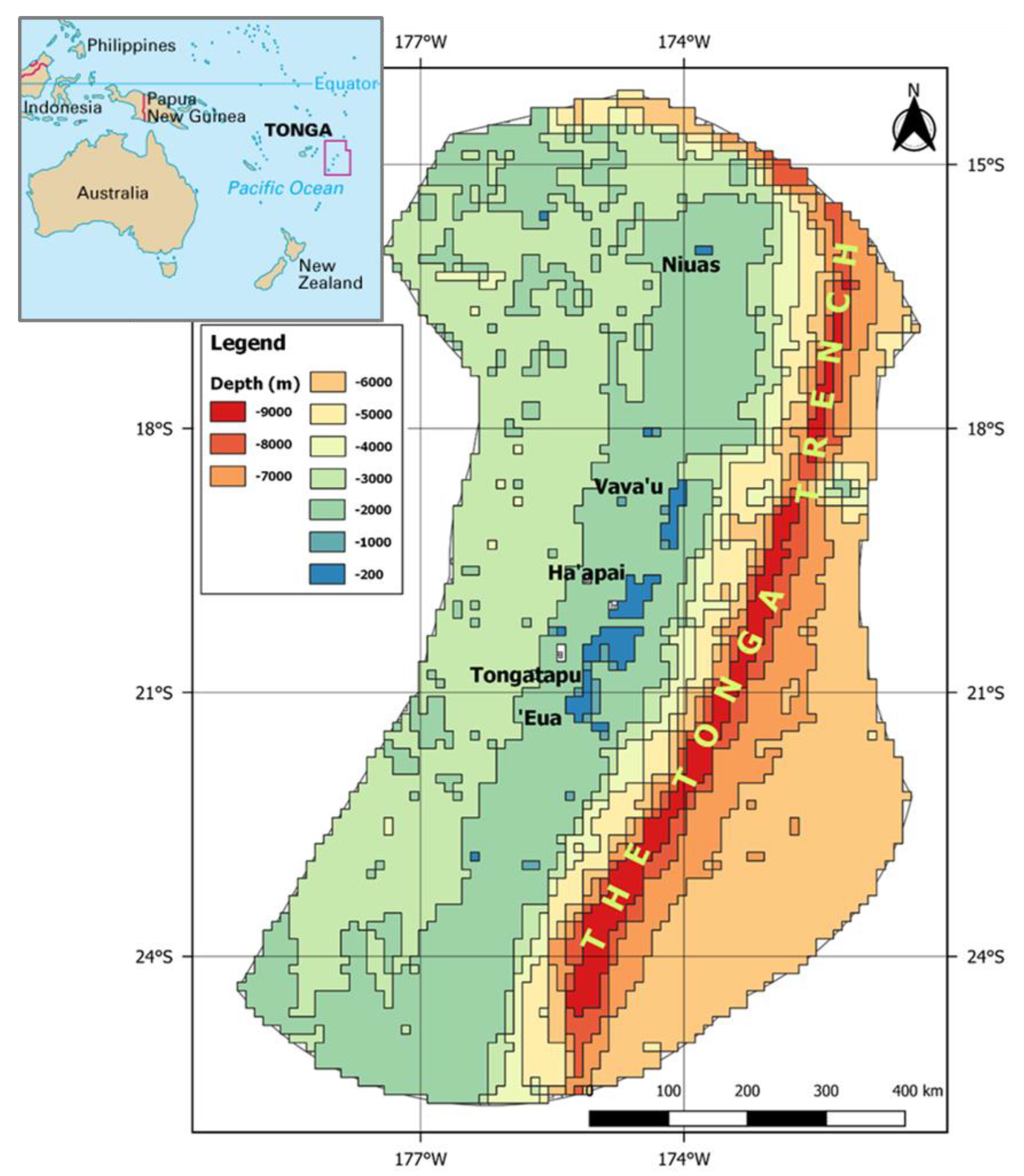
Figure 1. Bathymetry for the study region (EEZ of Tonga). Data aggregated to coarser resolution of 0.3 degree (~20 NM).
Diversity 15 01091 g001
Figure 2. Histograms of the distribution of CPUE (million tons per number of hooks) of albacore, bigeye, skipjack, and yellowfin for the duration of the study period of this study, 2002–2018, of the Tonga tuna fisheries within the EEZ, longitude 171.31 °   W 179.10 °   W .
Diversity 15 01091 g002
Figure 3. Histograms of the distribution of the environmental data, sea surface chlorophyll frontal gradients (chl_grad), depth, sea surface chlorophyll (log_chl), sea surface temperature and sea surface temperature frontal gradients (sst_grad) for the duration of the study period of this study, 2002–2018 of the NOAA repository [33], taken within the EEZ, longitude 171.31 °   W 179.10 °   W .
Diversity 15 01091 g003
Figure 4. The partial effects for covariates chl_grad, depth, Chl-a, SST, sst_grad, month and year for albacore, bigeye, skipjack, and yellowfin, respectively, within the EEZ of Tonga, longitude 171.31 °   W 179.10 °   W .
Diversity 15 01091 g004
Figure 5. Index of relative importance (refer to Section 2.4) of predictors for the four tuna species in the EEZ of Tonga, longitude 171.31 °   W 179.10 °   W .
Diversity 15 01091 g005
Figure 6. Plots of posterior predictive distribution of the models for (A) albacore, (B) bigeye, (C) skipjack and (D) yellowfin in the EEZ of Tonga, longitude 171.31 °   W 179.10 °   W . Distribution of the observed data is shown in black whereas the distributions from multiple draws of the model are shown in gray. Distribution of the observed data is shown in black whereas the distributions from multiple draws of the model are shown in gray. Posterior predictive check is way of checking if the model fits the data. The expectation is that if the model fits the data well, repeated generation of the data from fitted model should have the same distribution as the response variable. The presence of any systematic deviation from between the observed distribution and that posterior draws from the model indicates problem with the fitted model [48]. In this case no issue was observed.
Diversity 15 01091 g006
Figure 7. Time-series of standardized indices of CPUE for the four tuna species in the EEZ of Tonga, longitude 171.31 °   W 179.10 °   W .
Diversity 15 01091 g007
Figure 8. Predicted distribution map for albacore tuna arranged quarterly. DJF: December, January, February; MAM: March, April, May; JJA: June, July, August; SON: September, October, November within the EEZ of Tonga, longitude 171.31 °   W 179.10 °   W .
Diversity 15 01091 g008
Figure 9. Predicted distribution map for bigeye tuna arranged quarterly. DJF: December, January, February; MAM: March, April, May; JJA: June, July, August; SON: September, October, November within the EEZ of Tonga, longitude 171.31 °   W 179.10 °   W .
Diversity 15 01091 g009
Figure 10. Predicted distribution map for skipjack tuna arranged quarterly. DJF: December, January, February; MAM: March, April, May; JJA: June, July, August; SON: September, October, November within the EEZ of Tonga, longitude 171.31 °   W 179.10 °   W .
Diversity 15 01091 g010
Figure 11. Predicted distribution map for yellowfin tuna arranged quarterly. DJF: December, January, February; MAM: March, April, May; JJA: June, July, August; SON: September, October, November within the EEZ, longitude 171.31 °   W 179.10 °   W of Tonga.
Diversity 15 01091 g011
Table 1. Performance of the seven models considered for albacore, bigeye, skipjack, and yellowfin in the EEZ of Tonga. The mean RMSE and mae (mean absolute error) of the test data are presented.
SpeciesFormsMean RMSEMean mae
Albacorecpue~s(sst,k = 3)11.9738.795
cpue~s(sst,k = 3) + s(log_chl,k = 3)11.8338.601
cpue~s(sst,k = 3) + s(log_chl,k = 3) + s(sst_grad,k = 3)11.8148.572
cpue~s(sst,k = 3) + s(log_chl,k = 3) + s(sst_grad,k = 3) + s(chl_grad,k = 3)11.7328.487
cpue~s(sst,k = 3) + s(log_chl,k = 3) + s(sst_grad,k = 3) + s(chl_grad,k = 3) + s(depth,k = 3)11.7038.434
cpue~s(sst,k = 3) + s(log_chl,k = 3) + s(sst_grad,k = 3) + s(chl_grad,k = 3) + s(depth,k = 3) + s(month,bs = ‘cc’)10.7227.574
cpue~s(sst,k = 3) + s(log_chl,k = 3) + s(sst_grad,k = 3) + s(chl_grad,k = 3) + s(depth,k = 3) + s(month,bs = ‘cc’) + year10.2937.213
Bigeyecpue~s(sst,k = 3)2.8031.864
cpue~s(sst,k = 3) + s(log_chl,k = 3)2.8021.861
cpue~s(sst,k = 3) + s(log_chl,k = 3) + s(sst_grad,k = 3)2.8031.862
cpue~s(sst,k = 3) + s(log_chl,k = 3) + s(sst_grad,k = 3) + s(chl_grad,k = 3)2.8001.859
cpue~s(sst,k = 3) + s(log_chl,k = 3) + s(sst_grad,k = 3) + s(chl_grad,k = 3) + s(depth,k = 3)2.7901.852
cpue~s(sst,k = 3) + s(log_chl,k = 3) + s(sst_grad,k = 3) + s(chl_grad,k = 3) + s(depth,k = 3) + s(month,bs = ‘cc’)2.7621.814
cpue~s(sst,k = 3) + s(log_chl,k = 3) + s(sst_grad,k = 3) + s(chl_grad,k = 3) + s(depth,k = 3) + s(month,bs = ‘cc’) + year2.7091.748
Skipjackcpue~s(sst,k = 3)0.7550.326
cpue~s(sst,k = 3) + s(log_chl,k = 3)0.7550.327
cpue~s(sst,k = 3) + s(log_chl,k = 3) + s(sst_grad,k = 3)0.7560.327
cpue~s(sst,k = 3) + s(log_chl,k = 3) + s(sst_grad,k = 3) + s(chl_grad,k = 3)0.7560.327
cpue~s(sst,k = 3) + s(log_chl,k = 3) + s(sst_grad,k = 3) + s(chl_grad,k = 3) + s(depth,k = 3)0.7560.327
cpue~s(sst,k = 3) + s(log_chl,k = 3) + s(sst_grad,k = 3) + s(chl_grad,k = 3) + s(depth,k = 3) + s(month,bs = ‘cc’)0.7490.321
cpue~s(sst,k = 3) + s(log_chl,k = 3) + s(sst_grad,k = 3) + s(chl_grad,k = 3) + s(depth,k = 3) + s(month,bs = ‘cc’) + year0.7400.288
Yellowfincpue~s(sst,k = 3)11.3266.998
cpue~s(sst,k = 3) + s(log_chl,k = 3)11.1826.853
cpue~s(sst,k = 3) + s(log_chl,k = 3) + s(sst_grad,k = 3)11.1876.855
cpue~s(sst,k = 3) + s(log_chl,k = 3) + s(sst_grad,k = 3) + s(chl_grad,k = 3)11.1566.821
cpue~s(sst,k = 3) + s(log_chl,k = 3) + s(sst_grad,k = 3) + s(chl_grad,k = 3) + s(depth,k = 3)11.1576.809
cpue~s(sst,k = 3) + s(log_chl,k = 3) + s(sst_grad,k = 3) + s(chl_grad,k = 3) + s(depth,k = 3) + s(month,bs = ‘cc’)10.8466.631
cpue~s(sst,k = 3) + s(log_chl,k = 3) + s(sst_grad,k = 3) + s(chl_grad,k = 3) + s(depth,k = 3) + s(month,bs = ‘cc’) + year10.1275.989
Table 2. Model summary for the best GAM model for the four species. The cumulative proportion of deviance explained (Cum. dev. explained) from the null model (a model with just an intercept term) to the full model is presented.
SpeciesVariableFormsCum. Dev. Explained
AlbacoreNULLcpue~1
sstcpue~s(sst,k = 4)1.642
log_chlcpue~s(sst,k = 4) + s(log_chl,k = 4)4.375
sst_gradcpue~s(sst,k = 4) + s(log_chl,k = 4) + s(sst_grad,k = 4)4.823
chl_gradcpue~s(sst,k = 4) + s(log_chl,k = 4) + s(sst_grad,k = 4) + s(chl_grad,k = 4)6.027
depthcpue~s(sst,k = 4) + s(log_chl,k = 4) + s(sst_grad,k = 4) + s(chl_grad,k = 4) + s(depth,k = 4)8.057
monthcpue~s(sst,k = 4) + s(log_chl,k = 4) + s(sst_grad,k =4) + s(chl_grad,k = 4) + s(depth,k = 4) + s(month,bs = ‘cc’)20.588
yearcpue~s(sst,k = 4) + s(log_chl,k = 4) + s(sst_grad,k = 4) + s(chl_grad,k =4) +s(depth,k = 4) + s(month,bs = ‘cc’) + year27.622
BigeyeNULLcpue~1
sstcpue~s(sst,k = 4)2.840
log_chlcpue~s(sst,k = 4) + s(log_chl, k = 4)3.025
sst_gradcpue~s(sst,k = 4) + s(log_chl,k = 4) + s(sst_grad,k = 4)3.047
chl_gradcpue~s(sst,k = 4) + s(log_chl,k = 4) + s(sst_grad,k = 4) + s(chl_grad,k = 4)3.283
depthcpue~s(sst,k = 4) + s(log_chl,k = 4) + s(sst_grad,k = 4) + s(chl_grad,k = 4) + s(depth,k = 4)4.251
monthcpue~s(sst,k = 4) + s(log_chl,k = 4) + s(sst_grad,k =4) + s(chl_grad,k = 4) + s(depth,k = 4) + s(month,bs = ‘cc’)6.788
yearcpue~s(sst,k = 4) + s(log_chl,k = 4) + s(sst_grad,k = 4) + s(chl_grad,k =4) + s(depth,k = 4) + s(month,bs = ‘cc’) + year12.183
SkipjackNULLcpue~1
sstcpue~s(sst,k = 4)2.419
log_chlcpue~s(sst,k = 4) + s(log_chl, k = 4)2.493
sst_gradcpue~s(sst,k = 4) + s(log_chl,k = 4) + s(sst_grad,k = 4)2.495
chl_gradcpue~s(sst,k = 4) + s(log_chl,k = 4) + s(sst_grad,k = 4) + s(chl_grad,k = 4)2.518
depthcpue~s(sst,k = 4) + s(log_chl,k = 4) + s(sst_grad,k = 4) + s(chl_grad,k = 4) + s(depth,k = 4)2.837
monthcpue~s(sst,k = 4) + s(log_chl,k = 4) + s(sst_grad,k = 4) + s(chl_grad,k = 4) + s(depth,k = 4) + s(month,bs = ‘cc’)7.568
yearcpue~s(sst,k = 4) +s(log_chl,k = 4) + s(sst_grad,k = 4) + s(chl_grad,k = 4) +s(depth,k = 4) + s(month,bs = ‘cc’) + year24.895
YellowfinNULLcpue~1
sstcpue~s(sst,k = 4)1.937
log_chlcpue~s(sst,k = 4) + s(log_chl, k = 4)4.876
sst_gradcpue~s(sst,k = 4) + s(log_chl,k = 4) + s(sst_grad,k = 4)4.916
chl_gradcpue~s(sst,k = 4) + s(log_chl,k = 4) + s(sst_grad,k = 4) + s(chl_grad,k = 4)5.455
depthcpue~s(sst,k = 4) + s(log_chl,k = 4) + s(sst_grad,k = 4) + s(chl_grad,k = 4) + s(depth,k = 4)5.731
monthcpue~s(sst,k = 4) + s(log_chl,k =4) + s(sst_grad,k = 4) + s(chl_grad,k = 4) + s(depth,k = 4) + s(month,bs = ‘cc’)10.986
yearcpue~s(sst,k = 4) + s(log_chl,k = 4) + s(sst_grad,k = 4) + s(chl_grad,k = 4) +s(depth,k = 4) + s(month,bs = ‘cc’) + year24.287
Disclaimer/Publisher’s Note: The statements, opinions and data contained in all publications are solely those of the individual author(s) and contributor(s) and not of MDPI and/or the editor(s). MDPI and/or the editor(s) disclaim responsibility for any injury to people or property resulting from any ideas, methods, instructions or products referred to in the content.