

Where Land and Water Meet: Making Amphibian Breeding Sites Attractive for Amphibians

 , and
, and
Abstract
1. Introduction
2. Materials and Methods
2.1. The Amphibian Monitoring Programme
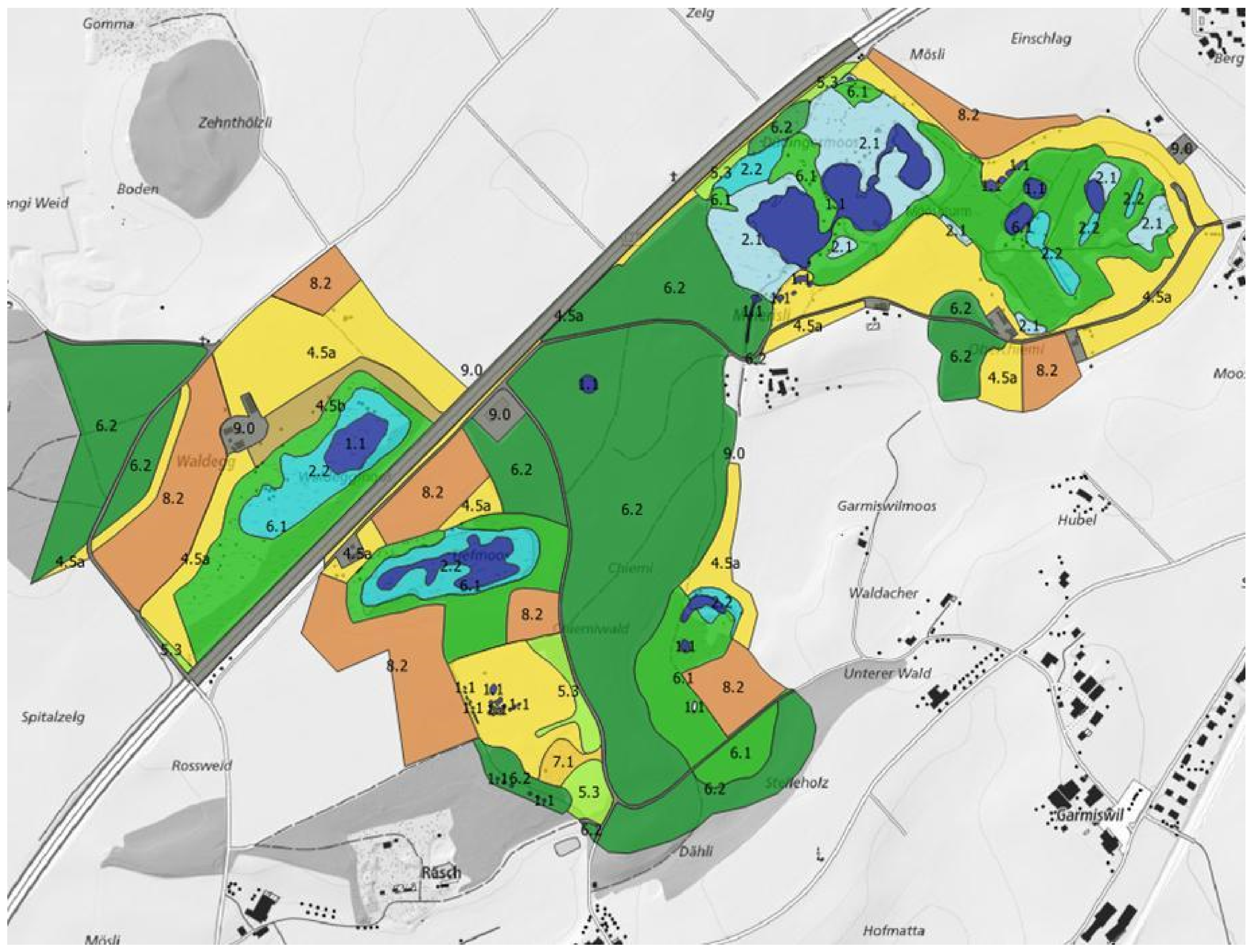
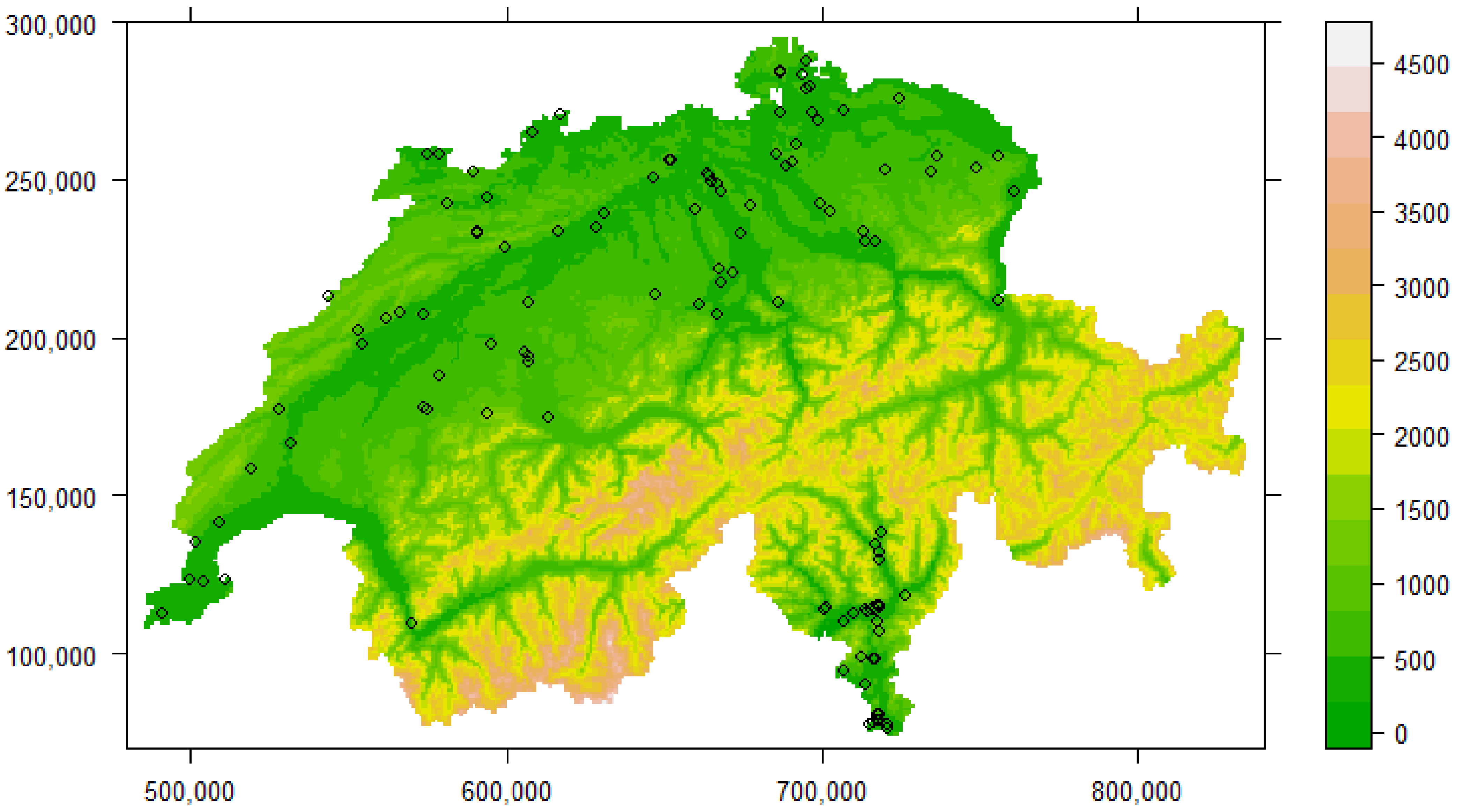
2.2. Habitat Mapping

| Variable Name | Meaning | Range |
|---|---|---|
| Past occurrence | Past population presence or absence (based on the records in the national database) | 0–1 |
| Connectivity | Connectivity, based on [30] (but modified) | 0–0.53 |
| Altitude | Altitude of the site [m] | 330–1460 |
| Total area of site | Total surface area of the site [ha] | 0.14–290.1 |
| Water | Area of water bodies within site (lentic and lotic) [ha] | 0–28.0 |
| Number of ponds | Number of ponds within site | 0–53 |
| Number of temporary ponds | Number of temporary ponds within site | 0–30 |
| Lentic aquatic habitat | Area of lentic aquatic habitats within site (a subset of “water”) [ha] | 0–27.2 |
| Built | Area of built area within site (e.g., surface of landfills, buildings, and roads) [ha] | 0–15.7 |
| Wetland | Area of wetlands within site (surface of artificial shores, reed beds, marshland, wet meadows, and bogs) [ha] | 0–90.9 |
| Meadow | Area of meadows within site (surface of meadows, and pastures) [ha] | 0–34.9 |
| Shrubs and tall forbs | Area of shrubs and tall herbs within site [ha] | 0–20.4 |
| Forest | Area of forests within site (including plantations) [ha] | 0–227.5 |
| Field | Area of agricultural fields within sites (surface of cultivation of woody and herbaceous plants) [ha] | 0–65.5 |
| Ruderal | Area of pioneer vegetation in man-made disturbed areas [ha] | 0–23.4 |

2.3. Connectivity
2.4. Statistical Analyses
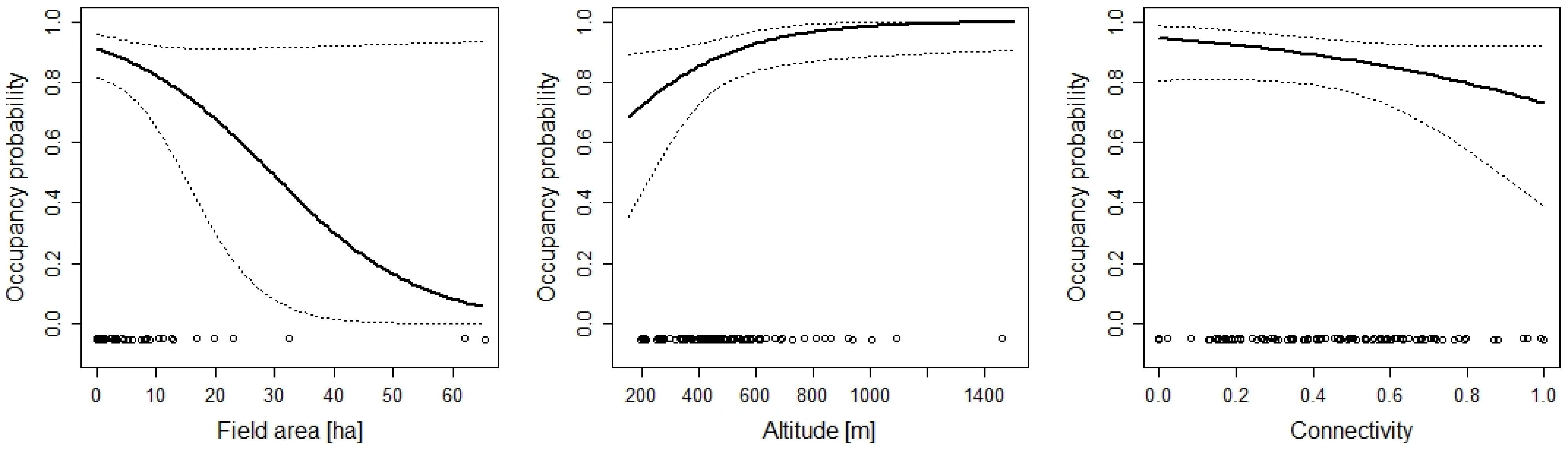
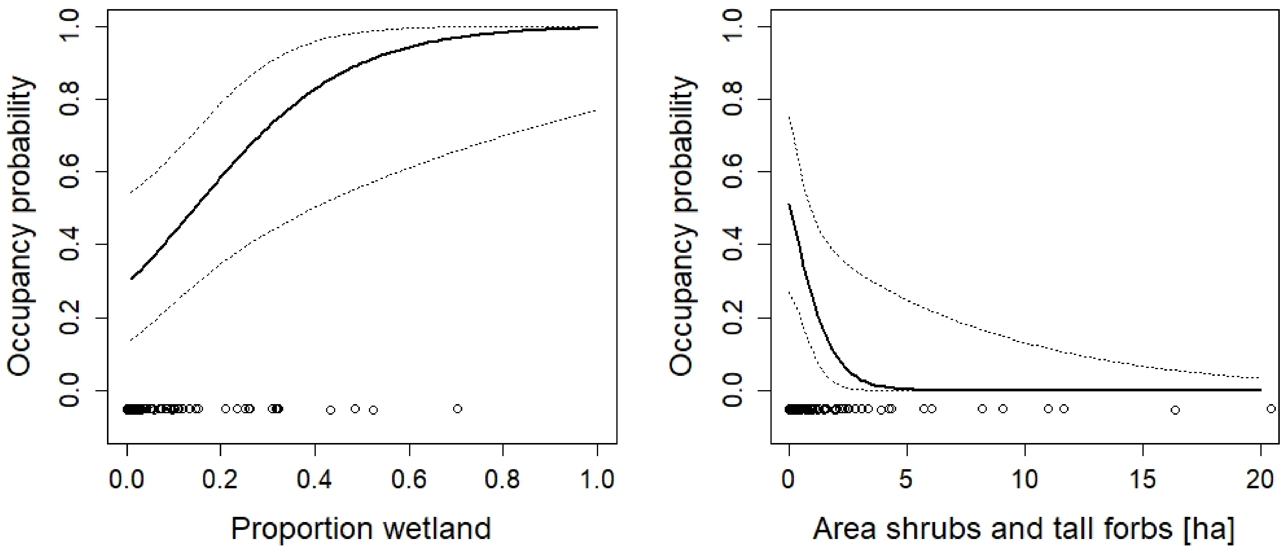
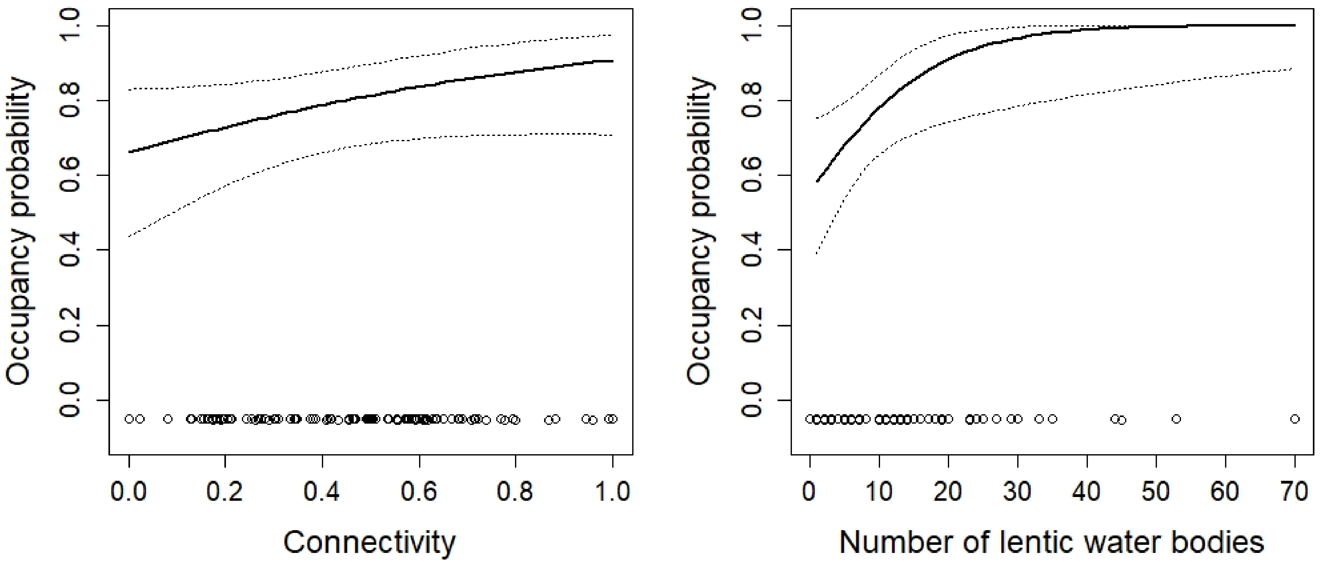
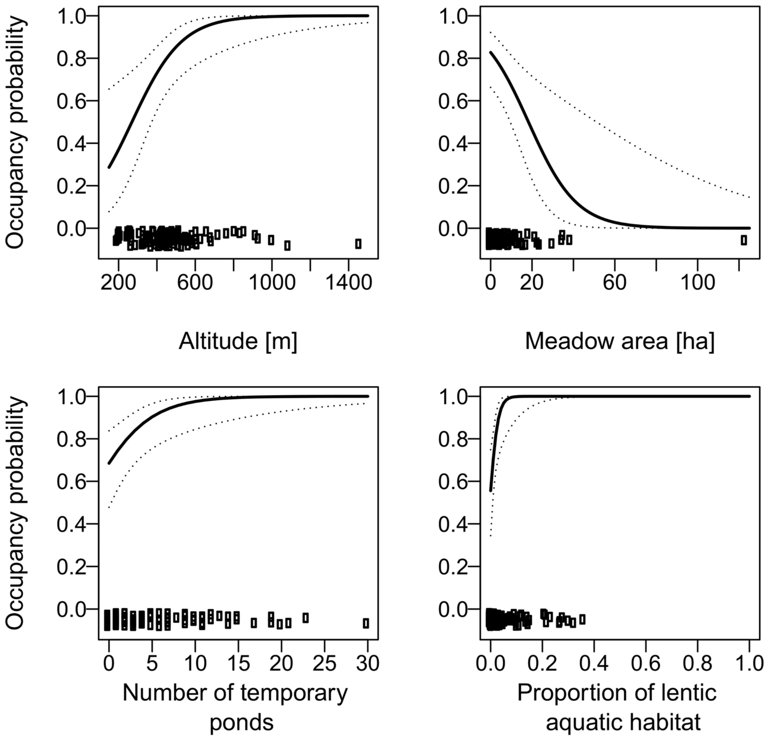
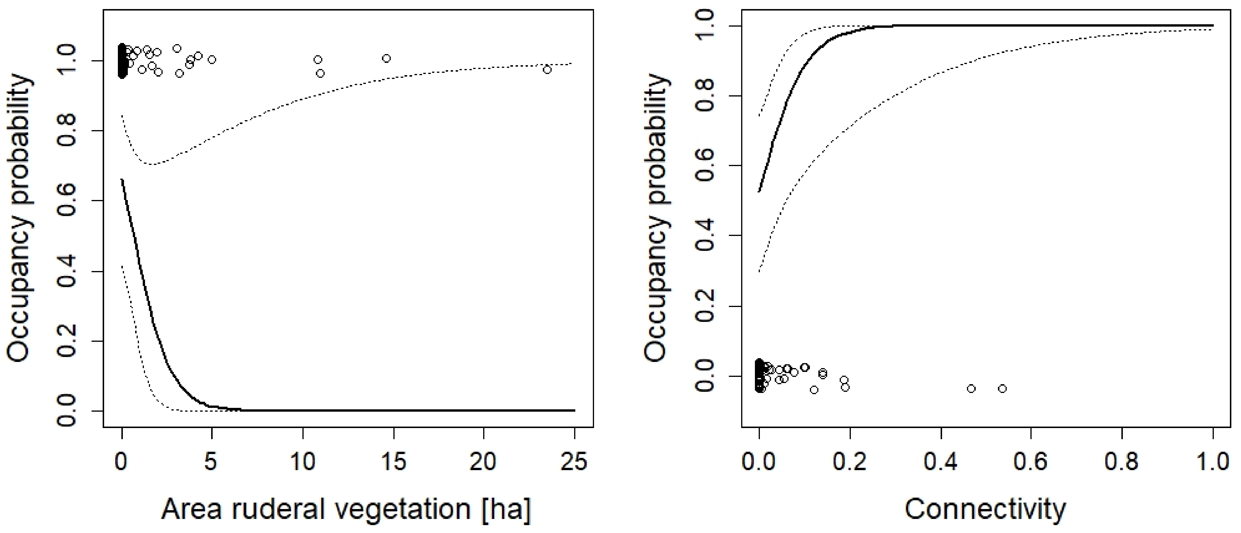
3. Results
4. Discussion
Author Contributions
Funding
Institutional Review Board Statement
Data Availability Statement
Acknowledgments
Conflicts of Interest
Appendix A

Appendix B

References
- Céréghino, R.; Biggs, J.; Oertli, B.; Declerck, S. The ecology of European ponds: Defining the characteristics of a neglected freshwater habitat. Hydrobiologia 2008, 597, 1–6. [Google Scholar] [CrossRef]
- Davies, B.; Biggs, J.; Williams, P.; Whitfield, M.; Nicolet, P.; Sear, D.; Bray, S.; Maund, S. Comparative biodiversity of aquatic habitats in the European agricultural landscape. Agric. Ecosyst. Environ. 2008, 125, 1–8. [Google Scholar] [CrossRef]
- Reid, A.J.; Carlson, A.K.; Creed, I.F.; Eliason, E.J.; Gell, P.A.; Johnson, P.T.J.; Kidd, K.A.; MacCormack, T.J.; Olden, J.D.; Ormerod, S.J.; et al. Emerging threats and persistent conservation challenges for freshwater biodiversity. Biol. Rev. 2019, 94, 849–873. [Google Scholar] [CrossRef] [PubMed]
- Dudgeon, D.; Arthington, A.H.; Gessner, M.O.; Kawabata, Z.I.; Knowler, D.J.; Lévêque, C.; Naiman, R.J.; Prieur-Richard, A.H.; Soto, D.; Stiassny, M.L.J.; et al. Freshwater biodiversity: Importance, threats, status and conservation challenges. Biol. Rev. 2006, 81, 163–182. [Google Scholar] [CrossRef]
- Soulé, M.E. What is conservation biology? BioScience 1985, 35, 727–734. [Google Scholar]
- Arlettaz, R.; Schaub, M.; Fournier, J.; Reichlin, T.S.; Sierro, A.; Watson, J.E.M.; Braunisch, V. From publications to public actions: When conservation biologists bridge the gap between research and implementation. BioScience 2010, 60, 835–842. [Google Scholar] [CrossRef]
- Grant, E.H.C.; Muths, E.; Schmidt, B.R.; Petrovan, S.O. Amphibian conservation in the Anthropocene. Biol. Conserv. 2019, 236, 543–547. [Google Scholar] [CrossRef]
- Albert, J.S.; Destouni, G.; Duke-Sylvester, S.M.; Magurran, A.E.; Oberdorff, T.; Reis, R.E.; Winemiller, K.O.; Ripple, W.J. Scientists’ warning to humanity on the freshwater biodiversity crisis. Ambio 2021, 50, 85–94. [Google Scholar] [CrossRef]
- Flitcroft, R.; Cooperman, M.S.; Harrison, I.J.; Juffe-Bignoli, D.; Boon, P.J. Theory and practice to conserve freshwater biodiversity in the Anthropocene. Aquat. Conserv. 2019, 29, 1013–1021. [Google Scholar] [CrossRef]
- Harper, M.; Mejbel, H.S.; Longert, D.; Abell, R.; Beard, T.D.; Bennett, J.R.; Carlson, S.M.; Darwall, W.; Dell, A.; Domisch, S.; et al. Twenty-five essential research questions to inform the protection and restoration of freshwater biodiversity. Aquat. Conserv. 2021, 9, 2632–2653. [Google Scholar] [CrossRef]
- Leverington, F.; Costa, K.L.; Pavese, H.; Lisle, A.; Hockings, M. A global analysis of protected area management effectiveness. Environ. Manag. 2010, 46, 685–698. [Google Scholar] [CrossRef]
- Watson, J.E.M.; Dudley, N.; Segan, D.B.; Hockings, M. The performance and potential of protected areas. Nature 2014, 515, 67–73. [Google Scholar] [CrossRef]
- Wauchope, H.S.; Jones, J.G.P.; Geldmann, J.; Simmons, B.I.; Amano, T.; Blanco, D.E.; Fuller, R.A.; Johnston, A.; Langendoen, T.; Mundkur, T.; et al. Protected areas have a mixed impact on waterbirds, but management helps. Nature 2022, 605, 103–107. [Google Scholar] [CrossRef]
- Grant, E.H.C.; Miller, D.A.W.; Schmidt, B.R.; Adams, M.J.; Amburgey, S.M.; Chambert, T.; Cruickshank, S.S.; Fisher, R.N.; Green, D.M.; Hossack, B.R.; et al. Quantitative evidence for the effects of multiple drivers on continental-scale amphibian declines. Sci. Rep. 2016, 6, 25625. [Google Scholar] [CrossRef]
- Houlahan, J.E.; Findlay, C.S.; Schmidt, B.R.; Meyer, A.H.; Kuzmin, S.L. Quantitative evidence for global amphibian declines. Nature 2000, 404, 752–755. [Google Scholar] [CrossRef]
- Braunisch, V.; Home, R.; Pellet, J.; Arlettaz, R. Conservation science relevant to action: A research agenda identified and prioritized by practitioners. Biol. Conserv. 2012, 153, 201–210. [Google Scholar] [CrossRef]
- Wake, D.B.; Vredenburg, V.T. Are we in the midst of the sixth mass extinction? A view from the world of amphibians. Proc. Natl. Acad. Sci. USA 2008, 105, 11466–11473. [Google Scholar] [CrossRef]
- Smalling, K.L.; Eagles-Smith, C.A.; Katz, R.A.; Grant, E.H.C. Managing the trifecta of disease, climate, and contaminants: Searching for robust choices under multiple sources of uncertainty. Biol. Conserv. 2019, 236, 153–161. [Google Scholar] [CrossRef]
- Schmidt, B.R.; Zumbach, S. Amphibian conservation in Switzerland. In Amphibian Biology: Volume 11, Status of Conservation and Decline of Amphibians, Eastern Hemisphere, Part 5, Northern Europe; Heatwole, H., Wilkinson, J.W., Eds.; Pelagic Publishing: Exeter, UK, 2019; pp. 46–51. [Google Scholar]
- Dunning, J.B.; Danielson, B.J.; Pulliam, H.R. Ecological processes that affect populations in complex landscapes. Oikos 1992, 65, 169–175. [Google Scholar] [CrossRef]
- Pope, S.E.; Fahrig, L.; Merriam, H.G. Landscape complementation and metapopulation effects on leopard frog populations. Ecology 2000, 81, 2498–2508. [Google Scholar] [CrossRef]
- Schmidt, B.R.; Arlettaz, R.; Schaub, M.; Lüscher, B.; Kröpfli, M. Benefits and limits of comparative effectiveness studies in evidence-based conservation. Biol. Conserv. 2019, 236, 115–123. [Google Scholar] [CrossRef]
- Van Buskirk, J. Local and landscape influence on amphibian occurrence and abundance. Ecology 2005, 86, 1936–1947. [Google Scholar] [CrossRef]
- Denoel, M.; Ficetola, G.F. Conservation of newt guilds in an agricultural landscape of Belgium: The importance of aquatic and terrestrial habitats. Aquat. Conserv. 2008, 18, 714–728. [Google Scholar] [CrossRef]
- Indermaur, L.; Schaub, M.; Jokela, J.; Tockner, K.; Schmidt, B.R. Differential response to abiotic conditions and predation risk rather than competition avoidance determine breeding site selection by anurans. Ecography 2010, 33, 887–895. [Google Scholar] [CrossRef]
- Bergamini, A.; Ginzler, C.; Schmidt, B.R.; Bedolla, A.; Boch, S.; Ecker, K.; Graf, U.; Küchler, H.; Küchler, M.; Dosch, O.; et al. Zustand und Entwicklung der Biotope von nationaler Bedeutung: Resultate 2011–2017 der Wirkungskontrolle Biotopschutz Schweiz. WSL Ber. 2019, 85, 1–104. [Google Scholar]
- Cruickshank, S.S.; Ozgul, A.; Zumbach, S.; Schmidt, B.R. Quantifying population declines based on presence-only records for Red List assessments. Conserv. Biol. 2016, 30, 1112–1121. [Google Scholar] [CrossRef]
- Petrovan, S.O.; Schmidt, B.R. Volunteer conservation action data reveals large-scale and long-term negative population trends of a widespread amphibian, the Common toad (Bufo bufo). PLoS ONE 2016, 11, e0161943. [Google Scholar] [CrossRef]
- Adams, M.J.; Muths, E. Conservation research across scales in a national program: How to be relevant to local management yet general at the same time. Biol. Conserv. 2019, 236, 100–106. [Google Scholar] [CrossRef]
- Zanini, F.; Pellet, J.; Schmidt, B.R. The transferability of distribution models across regions: An amphibian case study. Divers. Distrib. 2009, 15, 469–480. [Google Scholar] [CrossRef]
- Van Buskirk, J. Permeability of the landscape matrix between amphibian breeding sites. Ecol. Evol. 2012, 2, 3160–3167. [Google Scholar] [CrossRef]
- Luqman, H.; Muller, R.; Vaupel, A.; Brodbeck, S.; Bolliger, J.; Gugerli, F. No distinct barrier effects of highways and a wide river on the genetic structure of the Alpine newt (Ichthyosaura alpestris) in densely settled landscapes. Conserv. Genet. 2018, 19, 673–685. [Google Scholar] [CrossRef]
- Cruickshank, S.S.; Schmidt, B.R.; Ginzler, C.; Bergamini, A. Local habitat measures derived from aerial pictures are not a strong predictor of amphibian occurrence and abundance. Basic Appl. Ecol. 2020, 45, 51–61. [Google Scholar] [CrossRef]
- Wellborn, G.A.; Skelly, D.K.; Werner, E.E. Mechanisms creating community structure across a freshwater habitat gradient. Annu. Rev. Ecol. Syst. 1996, 27, 337–363. [Google Scholar] [CrossRef]
- Van Buskirk, J. Habitat partitioning in European and North American pond-breeding frogs and toads. Divers. Distrib. 2003, 9, 399–410. [Google Scholar] [CrossRef]
- Indermaur, L.; Winzeler, T.; Schmidt, B.R.; Tockner, K.; Schaub, M. Differential resource selection within shared habitat types across spatial scales in sympatric toads. Ecology 2009, 90, 3430–3444. [Google Scholar] [CrossRef]
- Denton, J.S.; Hitchings, S.P.; Beebee, T.J.C.; Gent, A. A recovery program for the natterjack toad (Bufo calamita) in Britain. Conserv. Biol. 1997, 11, 1329–1338. [Google Scholar] [CrossRef]
- Jehle, R.; Arntzen, J.W. Post-breeding migrations of newts (Triturus cristatus and T. marmoratus) with contrasting ecological requirements. J. Zool. 2000, 251, 297–306. [Google Scholar] [CrossRef]
- BAFU. Monitoring und Wirkungskontrolle Biodiversität: Übersicht zu Nationalen Programmen und Anknüpfungspunkten; Bundesamt für Umwelt: Bern, Switzerland, 2020. [Google Scholar]
- Cruickshank, S.S.; Bergamini, A.; Schmidt, B.R. Estimation of breeding probability can make monitoring data more revealing: A case study of amphibians. Ecol. Appl. 2021, 31, e02357. [Google Scholar] [CrossRef]
- McDonald, T.L. Review of environmental monitoring methods: Survey designs. Environ. Monit. Assess. 2003, 85, 277–292. [Google Scholar] [CrossRef]
- MacKenzie, D.I.; Nichols, J.D.; Lachman, G.B.; Droege, S.; Royle, J.A.; Langtimm, C.A. Estimating site occupancy rates when detection probabilities are less than one. Ecology 2002, 83, 2248–2255. [Google Scholar] [CrossRef]
- Dodd, C.K., Jr. (Ed.) Amphibian Ecology and Conservation: A Handbook of Techniques; Oxford University Press: Oxford, UK, 2009. [Google Scholar]
- Gerner, T. Fang, Markierung und Beprobung von Freilebenden Wildtieren: Vollzugshilfe zur Überwachung der Bestände und bei Erfolgskontrollen; Bundesamt für Umwelt: Bern, Switzerland, 2018. [Google Scholar]
- Delarze, R.; Gonseth, Y.; Eggenberg, S.; Vust, M. Lebensräume der Schweiz; Ott Verlag: Bern, Switzerland, 2015. [Google Scholar]
- Augustin, N.H.; Mugglestone, M.A.; Buckland, S.T. An autologistic model for the spatial distribution of wildlife. J. Appl. Ecol. 1996, 33, 339–347. [Google Scholar] [CrossRef]
- Fiske, I.; Chandler, R. unmarked: An R package for fitting hierarchical models of wildlife occurrence and abundance. J. Stat. Softw. 2011, 43, 1–23. [Google Scholar] [CrossRef]
- R Core Team. R: A Language and Environment for Statistical Computing; R Foundation for Statistical Computing: Vienna, Austria, 2020; Available online: https://www.R-project.org/ (accessed on 2 October 2022).
- Borgula, A.; Fallot, P.; Ryser, J. Inventar der Amphibienlaichgebiete von Nationaler Bedeutung: Schlussbericht; Bundesamt für Umwelt, Wald und Landschaft: Bern, Switzerland, 1994. [Google Scholar]
- Franklin, A.B.; Shenk, T.M.; Anderson, D.R.; Burnham, K.P. Statistical model selection: An alternative to null hypothesis testing. In Modeling in Natural Resource Management; Shenk, T.M., Franklin, A.B., Eds.; Island Press: Washington, DC, USA, 2001; pp. 75–90. [Google Scholar]
- Hooten, M.; Cooch, E.G. Comparing Ecological Models. In Quantitative Analysis in Wildlife Science; Brennan, L.A., Tri, A.N., Marcot, B.C., Eds.; Johns Hopkins University Press: Baltimore, MD, USA, 2019; pp. 63–76. [Google Scholar]
- Colegrave, N.; Ruxton, G.D. Confidence intervals are a more useful complement to nonsignificant tests than are power calculations. Behav. Ecol. 2003, 14, 446–450. [Google Scholar] [CrossRef]
- Meyer, A.; Zumbach, S.; Schmidt, B.; Monney, J.C. Auf Schlangenspuren und Krötenpfaden: Amphibien und Reptilien der Schweiz; Haupt: Bern, Switzerland, 2009. [Google Scholar]
- Schmidt, B.R. Are hybridogenetic frogs cyclical parthenogens? Trends Ecol. Evol. 1993, 8, 271–273. [Google Scholar] [CrossRef]
- Dubey, S.; Leuenberger, J.; Perrin, N. Multiple origins of invasive and ‘native’ water frogs (Pelophylax spp.) in Switzerland. Biol. J. Linn. Soc. 2014, 112, 442–449. [Google Scholar] [CrossRef]
- Stumpel, A.H.P.; van der Voet, H. Characterizing the suitability of new ponds for amphibians. Amphib. Reptil. 1998, 19, 125–142. [Google Scholar] [CrossRef]
- Oldham, R.S.; Keeble, J.; Swan, M.J.S.; Jeffcote, M. Evaluating the suitability of habitat for the great crested newt (Triturus cristatus). Herpetol. J. 2000, 10, 143–155. [Google Scholar]
- Denoel, M.; Lehmann, A. Multi-scale effect of landscape processes and habitat quality on newt abundance: Implications for conservation. Biol. Conserv. 2006, 130, 495–504. [Google Scholar] [CrossRef]
- Indermaur, L.; Schmidt, B.R. Quantitative recommendations for amphibian terrestrial habitat conservation derived from habitat selection behaviour. Ecol. Appl. 2011, 21, 2548–2554. [Google Scholar] [CrossRef][Green Version]
- Shulse, C.D.; Semlitsch, R.D.; Trauth, K.M.; Gardner, J.E. Testing wetland features to increase amphibian reproductive success and species richness for mitigation and restoration. Ecol. Appl. 2012, 22, 1675–1688. [Google Scholar] [CrossRef]
- Unglaub, B.; Steinfartz, S.; Kühne, D.; Haas, A.; Schmidt, B.R. The relationships between habitat suitability, population size and body condition in a pond-breeding amphibian. Basic Appl. Ecol. 2018, 27, 20–29. [Google Scholar] [CrossRef]
- Unglaub, B.; Cayuela, H.; Schmidt, B.R.; Preissler, K.; Glos, J.; Steinfartz, S. Context-dependent dispersal determines relatedness and genetic structure in a patchy amphibian population. Mol. Ecol. 2021, 30, 5009–5028. [Google Scholar] [CrossRef]
- Brown, J.H. Macroecology; University of Chicago Press: Chicago, IL, USA, 1995. [Google Scholar]
- Pellet, J.; Fleishman, E.; Dobkin, D.S.; Gander, A.; Murphy, D.D. An empirical evaluation of the area and isolation paradigm of metapopulation dynamics. Biol. Conserv. 2007, 136, 483–495. [Google Scholar] [CrossRef]
- Prugh, L.R.; Hodges, K.E.; Sinclair, A.R.E.; Brashares, J. Effect of habitat area and isolation on fragmented animal populations. Proc. Natl. Acad. Sci. USA 2008, 105, 20770–20775. [Google Scholar] [CrossRef]
- Blab, J. Biologie, Ökologie und Schutz von Amphibien; Kilda-Verlag: Warendorf, Germany, 1986; Volume 18, 150p. [Google Scholar]
- Schmidt, B.R. Steps towards better amphibian conservation. Anim. Conserv. 2008, 11, 469–471. [Google Scholar] [CrossRef]
- Riva, F.; Fahrig, L. The disproportionately high value of small patches for biodiversity conservation. Conserv. Lett. 2022, 15, e12881. [Google Scholar] [CrossRef]
- Cayuela, H.; Schmidt, B.R.; Weinbach, A.; Besnard, A.; Joly, P. Multiple density-dependent processes shape the dynamics of a spatially structured amphibian population. J. Anim. Ecol. 2019, 88, 164–177. [Google Scholar] [CrossRef]
- Joly, P.; Miaud, C.; Lehmann, A.; Grolet, O. Habitat matrix effects on pond occupancy in newts. Conserv. Biol. 2001, 15, 239–248. [Google Scholar] [CrossRef]
- Churko, G.; Kienast, F.; Bolliger, J. A multispecies assessment to identify the functional connectivity of amphibians in a human-dominated landscape. ISPRS Int. J. Geo-Inf. 2020, 9, 287. [Google Scholar] [CrossRef]
- Moor, H.; Bergamini, A.; Vorburger, C.; Holderegger, R.; Bühler, C.; Egger, S.; Schmidt, B.R. Bending the curve: Simple but massive conservation action leads to landscape-scale recovery of amphibians. Proc. Natl. Acad. Sci. USA 2022, 119. in press. [Google Scholar] [CrossRef]
- Calhoun, A.J.K.; Arrigoni, J.; Brooks, R.P.; Hunter, M.L.; Richter, S.C. Creating successful vernal pools: A literature review and advice for practitioners. Wetlands 2014, 34, 1027–1038. [Google Scholar] [CrossRef]
- Pellet, J. Temporäre Gewässer für gefährdete Amphibien schaffen—Leitfaden für die Praxis. Beiträge zum Naturschutz in der Schweiz 2014, 35, 1–25. [Google Scholar]
- Schmidt, B.R.; Zumbach, S.; Tobler, U.; Lippuner, M. Amphibien brauchen temporäre Gewässer. Z. Feldherpetol. 2015, 22, 137–150. [Google Scholar]
- Beebee, T.J.C.; Denton, J.S.; Buckley, J. Factors affecting population densities of adult natterjack toads Bufo calamita in Britain. J. Appl. Ecol. 1996, 33, 263–268. [Google Scholar] [CrossRef]
- Cayuela, H.; Monod-Broca, B.; Lemaître, J.-F.; Besnard, A.; Gippet, J.M.W.; Schmidt, B.R.; Romano, A.; Hertach, T.; Angelini, C.; Canessa, S.; et al. Compensatory recruitment allows amphibian population persistence in anthropogenic habitats. Proc. Natl. Acad. Sci. USA 2022, 119, e2206805119. [Google Scholar] [CrossRef]
- Barandun, J.; Reyer, H.-U. Reproductive ecology of Bombina variegata: Development of eggs and larvae. J. Herpetol. 1997, 31, 107–110. [Google Scholar] [CrossRef]
- Laciak, M.; Zajac, T.; Adamski, P.; Bielanski, W.; Cmiel, A.; Laciak, T.; Lipinska, A. Small monsters: Insect predation limits reproduction of yellow-bellied toad Bombina variegata to ponds in their earliest successional stage. Aquat. Conserv. 2022, 32, 817–831. [Google Scholar] [CrossRef]
- Semlitsch, R.D. Principles for management of aquatic-breeding amphibians. J. Wildl. Manag. 2000, 64, 615–631. [Google Scholar] [CrossRef]
- McCaffery, R.M.; Eby, L.A.; Maxell, B.A.; Corn, P.S. Breeding site heterogeneity reduces variability in frog recruitment and population dynamics. Biol. Conserv. 2014, 170, 169–176. [Google Scholar] [CrossRef]
- Stokes, D.L.; Messerman, A.F.; Cook, D.G.; Stemble, L.R.; Meisler, J.A.; Searcy, C.A. Saving all the pieces: An inadequate conservation strategy for an endangered amphibian in an urbanizing area. Biol. Conserv. 2021, 262, 109320. [Google Scholar] [CrossRef]


| Species | Variable | Coefficient | 95% CI |
|---|---|---|---|
| Alytes obstetricans | Past occurrence | 2.15 | 0.69, 3.61 |
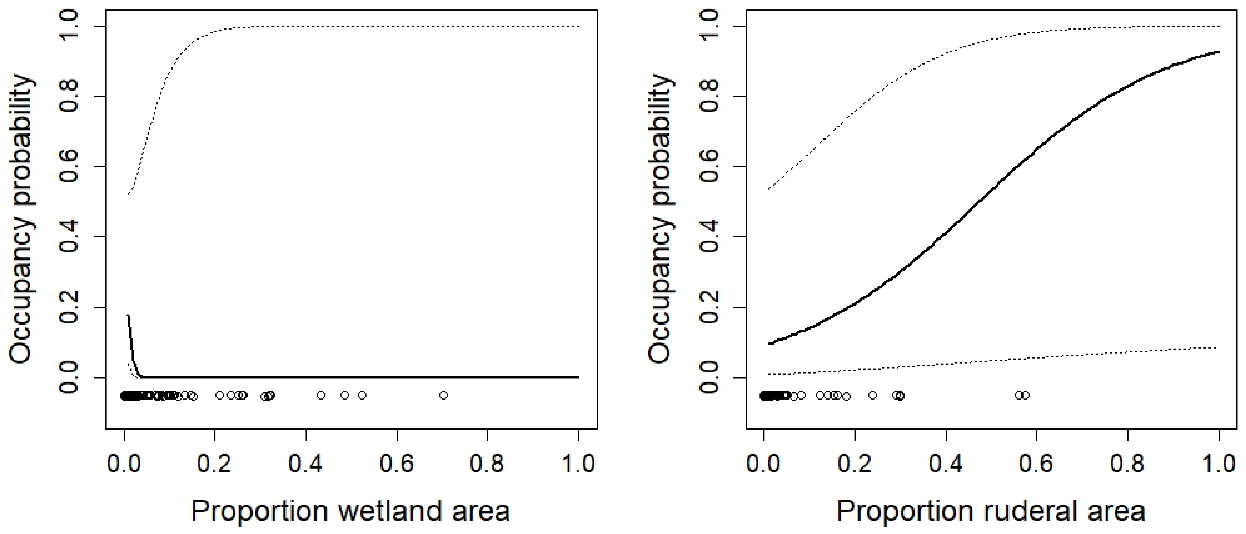
| Proportion wetland | −1.43 | −3.10, 0.22 | |
| Proportion ruderal vegetation | 0.048 | 0.002, 0.09 | |
| Bombina variegata | Past occurrence | 2.41 | 1.08, 3.75 |
| Number of temporary ponds | 0.10 | 0.006, 0.19 | |
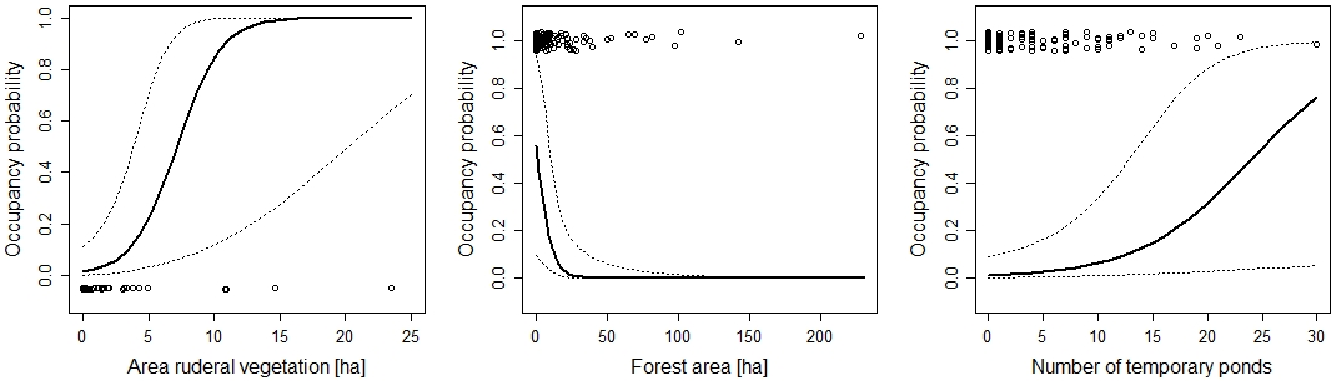
| Proportion ruderal vegetation | 0.07 | 0.02, 0.12 | |
| Area of forest | 0.01 | 0.002, 0.03 | |
| Bufo bufo | Past occurrence | 1.28 | 0.32, 2.24 |
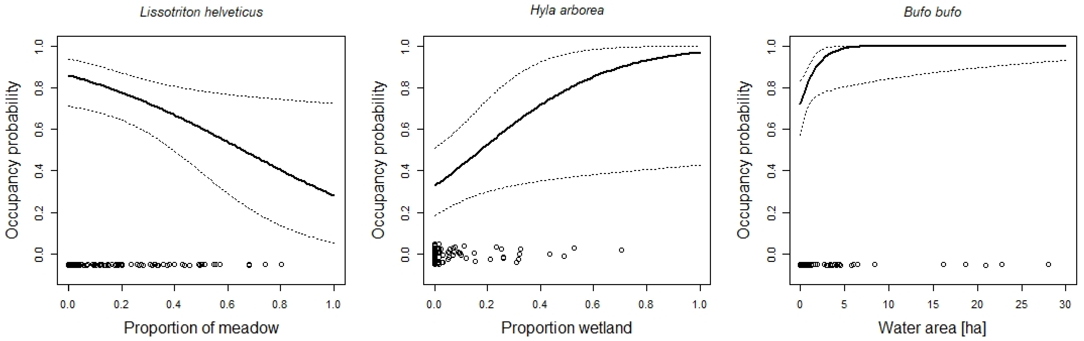
| Area of water | 0.68 | 0.04, 1.32 | |
| Epidalea calamita | Past occurrence | −0.20 | −2.21, 1.80 |
| Number of temporary ponds | 0.19 | 0.03, 0.35 | |
| Area of ruderal vegetation | 0.59 | 0.16, 1.02 | |
| Area of forest | −0.18 | −0.34, −0.02 | |
| Hyla arborea | Past occurrence | 1.22 | 0.25, 2.19 |
| Proportion wetland | 0.04 | 0.003, 0.07 | |
| Hyla intermedia | Past occurrence | −0.912 | −3.37, 0.42 |
| Connectivity | −3.671 | −7.76, 0.42 | |
| Area of lentic aquatic habitat | 14.58 | −14.01,43.17 | |
| Ichthyosaura alpestris | Past occurrence | 3.75 | 2.47, 5.02 |
| Connectivity | −1.84 | −4.31, 0.62 | |
| Altitude | 0.003 | 0.0003, 0.007 | |
| Area of fields | −0.07 | −0.16, 0.01 | |
| Lissotriton helveticus | Past occurrence | 3.25 | 2.20, 4.29 |
| Proportion meadows | −0.02 | −0.05, −0.003 | |
| Lissotriton vulgaris | Past occurrence | 1.24 | 0.09, 2.39 |
| Proportion wetlands | 0.06 | 0.01, 0.10 | |
| Area of shrubs and tall forbs | −1.16 | −2.18, −0.14 | |
| Pelophylax frogs | Past occurrence | 0.20 | −0.78, 1.18 |
| Connectivity | 1.61 | −0.28, 3.51 | |
| Number of ponds | 0.10 | 0.01, 0.19 | |
| Rana dalmatina | Past occurrence | 2.72 | 1.57, 3.87 |
| Connectivity | −0.11 | −2.31, 2.08 | |
| Altitude | −0.005 | −0.009, −0.001 | |
| Area of fields | 0.11 | 0.01, 0.22 | |
| Rana temporaria | Connectivity | 2.03 | −0.48, 4.56 |
| Altitude | 0.007 | 0.002, 0.013 | |
| Number of temporary ponds | 0.29 | 0.07, 0.50 | |
| Area of lentic aquatic habitat | 0.63 | 0.14, 1.12 | |
| Area of meadows | −0.08 | −0.14, −0.02 | |
| Triturus carnifex | Past occurrence | −0.5 | −2.43, 1.41 |
| Proportion forest | 0.04 | −1.18, 0.08 | |
| Number of temporary ponds | 0.33 | 0.02, 0.63 | |
| Triturus cristatus | Past occurrence | 1.63 | 0.44, 2.83 |
| Connectivity | 19.39 | 4.38, 34.37 | |
| Area of ruderal vegetation | −0.98 | −2.15, 0.17 |
Publisher’s Note: MDPI stays neutral with regard to jurisdictional claims in published maps and institutional affiliations. |
© 2022 by the authors. Licensee MDPI, Basel, Switzerland. This article is an open access article distributed under the terms and conditions of the Creative Commons Attribution (CC BY) license (https://creativecommons.org/licenses/by/4.0/).
Share and Cite
Siffert, O.; Pellet, J.; Ramseier, P.; Tobler, U.; Bergamini, A.; Schmidt, B.R. Where Land and Water Meet: Making Amphibian Breeding Sites Attractive for Amphibians. Diversity 2022, 14, 834. https://doi.org/10.3390/d14100834
Siffert O, Pellet J, Ramseier P, Tobler U, Bergamini A, Schmidt BR. Where Land and Water Meet: Making Amphibian Breeding Sites Attractive for Amphibians. Diversity. 2022; 14(10):834. https://doi.org/10.3390/d14100834
Chicago/Turabian StyleSiffert, Océane, Jérôme Pellet, Petra Ramseier, Ursina Tobler, Ariel Bergamini, and Benedikt R. Schmidt. 2022. "Where Land and Water Meet: Making Amphibian Breeding Sites Attractive for Amphibians" Diversity 14, no. 10: 834. https://doi.org/10.3390/d14100834
APA StyleSiffert, O., Pellet, J., Ramseier, P., Tobler, U., Bergamini, A., & Schmidt, B. R. (2022). Where Land and Water Meet: Making Amphibian Breeding Sites Attractive for Amphibians. Diversity, 14(10), 834. https://doi.org/10.3390/d14100834