Abstract
The spatially autocorrelated patterns of biodiversity can be an important determinant of ecological processes, functions and delivery of services across spatial scales. Therefore, understanding disturbance effects on spatial autocorrelation in biodiversity is crucial for conservation and restoration planning but remains unclear. In a survey of disturbance versus spatial patterns of biodiversity literature from forests, grasslands and savannah ecosystems, we found that habitat disturbances generally reduce the spatial autocorrelation in species diversity on average by 15.5% and reduce its range (the distance up to which autocorrelation prevails) by 21.4%, in part, due to disturbance-driven changes in environmental conditions, dispersal, species interactions, or a combination of these processes. The observed effect of disturbance, however, varied markedly among the scale of disturbance (patch-scale versus habitat-scale). Surprisingly, few studies have examined disturbance effects on the spatial patterns of functional diversity, and the overall effect was non-significant. Despite major knowledge gaps in certain areas, our analysis offers a much-needed initial insights into the disturbance-driven changes in the spatial patterns of biodiversity, thereby setting the ground for informed discussion on conservation and promotion of spatial heterogeneity in managing natural systems under a changing world.
1. Introduction
Habitat disturbance is a major driver of biodiversity change in natural and semi-natural ecosystems worldwide [1,2,3]. The research foci of disturbance-driven biodiversity change, and retrospective conservation and restoration efforts, have largely been prioritized towards the average values of biodiversity [4]. However, the replicate observations from which an average value is derived may not be always spatially independent [5,6]. Similar abiotic condition, neighborhood biotic interactions and patchy dispersal, for example, could generate positively or negatively correlated patterns of biodiversity distribution within a habitat (see Appendix A for further details). Those spatially correlated patterns of biodiversity, once treated as a statistical nuisance, are now considered crucial for maintaining ecological processes, functions and delivery of services across spatial scales [7,8,9,10,11,12,13]. Spatial continuity in forest and grassland biodiversity, for instance, may promote lateral flow of matter and energy, pollination, seed dispersal, or animal movement across spatial scales, and it may also increase the risk of disease spread [13,14]. Spatially aggregated patterns of biodiversity have also been shown to enhance ecosystem functioning compared to spatially random biodiversity patterns [10]. Therefore, if the spatial patterns of biodiversity are modified by disturbances [15,16], important processes, functions and delivery of services across spatial scales are expected to be compromised [13,17]. Understanding the nature and extent to which disturbances may impact the spatial patterns of biodiversity is, thus, crucial for conservation and restoration planning [6,17,18,19,20], but remains unclear.
Conceptually, disturbances can inflict serious consequences for spatial biodiversity patterns via its effects on site environmental condition, dispersal or species interactions that shape species’ spatial distribution and community composition, and in turn, shape the spatial patterns of biodiversity [16,21,22]. That means, when site environmental conditions, dispersal or species interaction patterns are affected by disturbance, species’ spatial distribution and community composition are expected to be modified, and when species’ spatial distribution or community composition are modified, spatial patterns of biodiversity are expected to be changed [15].
However, the direction and magnitude of disturbance-driven changes in the spatial patterns of biodiversity could depend on multiple factors, including the scale at which particular disturbances operate [17,21,23,24,25,26] and the type and intensity of disturbance. Of course, such effects may further depend on the spatial heterogeneity of the habitat template [26,27]. In a spatially patchy habitat (e.g., patch-matrix or mosaic), which is usually characterized by a patchy-type of spatial pattern, disturbances operating at the scale of a habitat may weaken or homogenize the within-habitat biotic and abiotic heterogeneity [24]. This may lead to a shift from patchy-type to gradient- or to random-type of spatial patterns [23], or may lead to an increase in the overall positive autocorrelation in biodiversity (Figure 1). Here, a patchy-type of spatial pattern can be defined as the pattern where the overall autocorrelation is significant, but the shape of the pattern is somewhat wavy. A gradient-type of spatial pattern can be defined as the pattern where the overall autocorrelation is significant, but the shape of the pattern is somewhat an accelerating or decelerating line; and a random-type of pattern can be attributed to the abundance of fine-scale patches or local spatial structures, resulting in an overall non-significant spatial autocorrelation in biodiversity. However, in the same patch-matrix or mosaic habitat, disturbances, operating at the scale of a microhabitat patch, may increase the within-habitat biotic and abiotic heterogeneity [24,28], causing a decrease in overall positive spatial autocorrelation or generate a more patchy-type of post-disturbance patterns in biodiversity. In a gradient-dominated or homogeneous habitat with a gradient- or a random-type of spatial pattern, disturbances operating at the scale of a habitat may not affect the overall spatial pattern. Whereas, disturbances operating at the scale of a microhabitat patch may create new patches (i.e., shift from a gradient-type or a random-type to a patchy-type pattern) [23] or a decrease in the overall spatial autocorrelation in biodiversity (Figure 1). Yet, these aspects of disturbance and resultant changes in the categories of spatial patterns are rarely considered explicitly in disturbance versus spatial patterns of biodiversity studies.
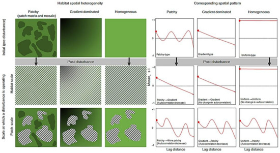
Figure 1.
Conceptual diagram illustrating disturbance-driven changes in the spatial autocorrelation of biodiversity. The hatched lines in the figures indicate the spatial scale of disturbance, either over the entire habitat (when the hatched lines spread over the entire area) or within a patch (when the lines are spread within selected area). The corresponding spatial patterns (cf. spatial autocorrelation) are shown (right hand side of the figure) in the context of Moran’s I.
Moreover, disturbances affecting biotic assemblage directly should affect the spatial patterns of biodiversity strongly, while disturbances affecting the biotic assemblage indirectly should affect the spatial pattern weakly and somewhat gradually [21]. That means, the above-mentioned disturbance-driven changes in the spatial patterns of biodiversity may depend on the types of disturbance. For instance, grazing, forest harvesting, human-induced fire, or other types of disturbance often impacts the abiotic and biotic properties of ecological systems in its own ways: Grazing disturbance generally removes biomass, forest harvesting removes biomass, as well as disturbs the ground and fire disturbance involves removal of biomass and inputs of nutrients (through ashes). Ecological impacts of varying disturbance types may, thus, impact the spatial patterns of biodiversity differently.
Similarly, disturbance effects on the spatial patterns of different indices of species (e.g., presence, abundance, richness, evenness, diversity and composition) and functional diversity (e.g., abundance of certain functional groups, functional richness, functional evenness, functional divergence, functional diversity and mean values of individual traits) should vary markedly. Some indices of biodiversity, such as species abundance can be felt immediately, while the effects on other indices, such as richness or diversity may be felt gradually, especially when assembly processes come into play [15].
To date, relatively few studies have examined the effects of disturbance on the spatial autocorrelation in species or functional diversity indices, and most of these studies focused on particular disturbance types, scale of disturbance and indices of species or functional diversity. Not surprisingly, some studies have found disturbance-driven profound changes in the spatial patterns of some indices of species or functional diversity, while others have found slight or no change at all. To our knowledge, no attempt has been made to synthesize the response patterns of spatial patterns of biodiversity to disturbances or to explore the reasons underlying the variability in results between studies. Therefore, here, we present an initial synthesis examining the directionality, magnitude and causes of disturbance-driven changes in the spatial patterns (the intensity of spatial autocorrelation indicating spatial connectedness and spatial range indicating patch size) of species and functional diversity. We also examine whether the scale of disturbance may constrain the post-disturbance spatial patterns. While a spatial pattern can include both point and surface/lateral patterns [23], we emphasize the analysis of surface/lateral patterns, just to be consistent with the quadrat-based traditional approaches in community ecology.
2. Materials and Methods
2.1. Literature Search and Study Selection
We conducted a literature search in the Web of Science, Google Scholar and Scopus databases on December 6, 2020, using relevant key words such as ‘spatial pattern’, ‘spatial structure’, ‘spatial autocorrelation’, ‘spatial relationship’, ‘spatial heterogeneity’, ‘autocorrelation’, and ‘land use’, ‘disturbance’, ‘forest conversion’, ‘climate change’, ‘fire’, ‘grazing’, ‘invasion’, ‘insect attack’, ‘clear-cutting’, and ‘diversity’, ‘richness’, ‘evenness’ etc. That is, we looked for peer reviewed publications reporting the impacts of disturbance or land use changes on the spatial patterns of commonly used indices of species (presence, abundance, richness, evenness, diversity, composition) and functional diversity (richness, evenness, diversity and community weighted means of individual trait).
Our keyword search resulted in a total of 1609 papers. We read the titles and abstracts of those papers and removed 1537 papers because they were not relevant to the present study. We then read the remaining 72 papers thoroughly and identified papers that (i) compared the spatial patterns of biodiversity before, and after, disturbance or disturbed versus undisturbed habitats in a comparable setting, and (ii) measured the spatial pattern of at least one index of species or functional diversity. A total of 28 papers meet our selection criteria. We consulted the forward and backward citations of these papers and selected four additional papers following the two criteria mentioned above. We checked the papers for the possibility of duplicate data in multiple papers but did not find any such case. Finally, we selected a total of 32 papers [15,16,21,22,27,28,29,30,31,32,33,34,35,36,37,38,39,40,41,42,43,44,45,46,47,48,49,50,51,52,53,54] that we coded for detailed analysis and synthesis (Figure 2; data presented in Supplementary Materials).

Figure 2.
Map of the global distribution of studies from different ecosystems.
2.2. Data Extraction and Coding
For each paper selected for the analysis (N = 32), we extracted data regarding the intensity and range of spatial autocorrelation in disturbed versus undisturbed habitats, or pre- versus post-disturbances from text, tables, figures, or from raw data (when available). When results were reported graphically, we used WebPlotDigitizer (https://automeris.io/WebPlotDigitizer/; accessed date on 6 December 2020) to extract data from figures. For all papers, we recorded the geographical coordinates, ecosystem type (forests, grasslands or savannah), types of habitat spatial heterogeneity (heterogeneous, gradient and homogeneous), types of initial and final spatial patterns (patchy, gradient, homogeneous), disturbance type, and the scale at which a particular disturbance operates (habitat-scale versus patch-scale). Some of the qualitative information was not always explicit in each paper; therefore, we developed the following rules a priori to identify and classify studies consistently.
2.2.1. Classifying the Scale of Disturbance
Although all possible types of disturbance are individually of interest, sufficient evidence does not exist to accurately examine impacts along the full gradient of disturbance types. We therefore grouped disturbance types into four categories: (i) grazing, (ii) burning, (iii) forest harvesting and others, such as forest or grassland management disturbance and physiological stresses induced by environmental harshness. However, as illustrated in Figure 1, when a particular disturbance occurred/applied over the entire habitat, we coded that as habitat-scale disturbance, and when a particular disturbance type occurred/applied only within a sub-habitat or microhabitat patches, we coded them as patch-scale disturbance.
2.2.2. Classifying Habitat Spatial Heterogeneity, and Pre-Versus Post-Disturbance Spatial Pattern
Following Biswas and Wagner [26], we classified habitat spatial heterogeneity into four categories: patch-matrix (binary, habitat versus matrix), mosaic (different categories of habitat quality), gradient (quantitative scale of habitat quality without distinct categories), and homogeneous. However, for simplicity of interpretation, we merged the patch-matrix and mosaic categories of habitat spatial heterogeneity into a single category of patchy habitat. That is, when the study site description indicated the types of habitat configurations as habitat versus matrix or different types of habitat quality, we classified them as patchy habitat. When the study site description indicated the types of habitat configuration as gradients of habitat quality, we classified them as gradient dominated habitat; and when there is no mention of habitat quality, we consider them as homogeneous habitat.
To examine the effects of disturbance on the spatial patterns of biodiversity, we first coded each pattern into one of three categories (i.e., patchy, gradient, random), based on the correlogram, variogram or dissimogram. That is, when the presented correlogram, variogram or dissimogram for biodiversity showed a clear wavy pattern, we coded that as a patchy-type of pattern. As the presented correlogram, variogram or dissimogram showed somewhat straight, but accelerating or decelerating line, we coded them as a gradient-type pattern, and when there was no clear pattern, we coded them as random pattern. We repeated the same classification procedure for pre- versus post-disturbance, or comparable disturbed versus undisturbed habitats. We, then, classified the disturbance-driven changes in the spatial patterns of biodiversity into one of six possible categories as appropriate: (i) Patchy to random (P > R), (ii) gradient to random (G > R), (iii) random to patchy (R > P), (iv) gradient to patchy (G > P), (v) random to gradient (R > G) and (vi) no-change. Note that, non-change can occur in terms of patchy to patchy, gradient to gradient or random to random pattern for pre- versus post-disturbance, or disturbed versus undisturbed habitats
2.2.3. Classifying the Causes of Disturbance-Driven Changes in Spatial Patterns
Typically, disturbance-driven changes in the spatial patterns of biodiversity are expected to occur via changes in the patterns of environmental filtering, biotic interactions and dispersal [21]. We, thus, read each paper carefully and extracted the author’s explanations for the observed changes (or no change) in the spatial patterns of biodiversity. When more than one explanation was suggested by the authors, we recorded them as such [26]. Recognizing the considerable uncertainty in such interpretations using observational data, we used these explanation to understand the possible drivers rather than to test any hypothesis regarding spatial biodiversity change [55].
2.3. Data Analysis
To examine the impacts of disturbance on spatial connectedness (autocorrelation intensity) or patch size (spatial range) of species and functional diversity, we computed the natural log-response ratio (lnRR) in spatial autocorrelation intensity or patch size of species diversity and functional diversity for each disturbance treatment with respect to corresponding control as the effect size, which improves its statistical behaviour in meta-analyses [56]: lnRR = log(xt/xc). Where xt and xc are the autocorrelation intensities or spatial range in species or functional diversity, for disturbed habitat, and undisturbed (or post- and pre-disturbance) control, respectively.
In our data set, some records (23 entries) showed sign-change (i.e., change from positive to negative autocorrelation, and vice versa), so that log transformation of the response ratios for those record produced ‘NA’ values. To examine whether the exclusion of those records make any difference or not, we employed a non-parametric on-sample Wilcoxon signed rank test to examine whether the untransformed response ratio was significantly different from 1 or not [57]. We found the overall results consistent with, and without, log-transformation (i.e., with or without exclusion of these entries). Therefore, we took the parametric approach and continued our analysis with lnRR. While, meta-analysis calls for accounting for variation in the uncertainty of the estimated lnRR among studies, we were unable to do so because information on the variability of estimates, such as standard deviation or sample size was rarely reported (note that, the number of neighboring pairs used to compute spatial autocorrelation is the true sample size in this case). Therefore, we weighed all the observations equally like several other studies [55,58,59], even though some estimates were more precise than others.
To examine whether the observed effect depended on the scale of disturbance, we conducted a general linear model analysis, using lnRR as a response variable and the scale of disturbance as a predictor. Residual analysis indicated that the normality assumptions were met. While we conducted our analysis using lnRR, we back-transformed the overall effect size of lnRR to percent change, i.e., (e (lnRR)−1) × 100, for brevity and readability.
To examine whether the disturbance-driven changes in spatial patterns of biodiversity (i.e., P > R, G > R, R > P, G > P, R > G and no-change) depended on the scale of disturbance (habitat scale versus patch-scale), we performed a contingency table—based test. All statistical analyses were conducted in the statistical program R (version 4.0.2).
While the potential dependency of disturbance-driven changes in the spatial autocorrelation in species and functional diversity on disturbance type, intensity and indices of species and functional diversity were our main interests, there were insufficient studies (see state of the literature below) to draw any robust conclusions. We, thus, lumped different types of disturbance into a single category of disturbed habitat, and different indices of species or functional diversity into a single category of species or functional diversity.
3. Results
3.1. State of the Literature
Our meta-dataset included a total of 32 studies from grasslands (N = 22 studies), forests (N = 6) and savanna ecosystems (N = 4), published from 1984 to 16 October 2020 and spreading over 12 countries (Figure 2). Of which, 78% (N = 25) studies reported on a single or multiple indices of species diversity and 25% (N = 8) studies reported on different indices of functional diversity. About 56% (N = 18) of studies focused on habitat-scale disturbance, while 44% (N = 14) focused on patch-scale disturbance. About 53% of studies reported the initial spatial patterns of biodiversity as patchy, 19% gradient and 28% random. Most of the disturbances took place in the form of grazing (56%), while a small number of studies also focused on burning (22%), forest harvesting (13%), and other forms of disturbances, including physiological stress and grassland management (16%).
3.2. Patterns of Change in Spatial Autocorrelation (Spatial Connectedness)
Across disturbance types, scales of disturbance and indices of species diversity, habitat disturbance resulted on average 15.50% decline in spatial autocorrelation in species diversity (p = 0.03). However, such effects varied substantially among scale of disturbance (p < 0.01) (Figure 3A). For functional diversity, only few studies examined the disturbance effects on spatial patterns, and the overall effects were not significant (confidence interval overlaps zero in Figure 3B).
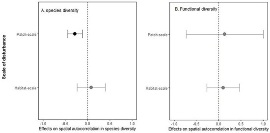
Figure 3.
Disturbance effects on spatial autocorrelation in species (A) and functional diversity (B) for patch-scale and habitat-scale disturbances. Shown in the figure is mean (solid point) and 95% confidence intervals (solid line). Statistically significant effects are shown in dark colour, and non-significant effects are shown in grey.
Due to the limited number of studies, we refrained from drawing any conclusions regarding the effects of disturbance type and intensity on spatial autocorrelation in species and functional diversity, or whether the observed effects vary among indices of biodiversity. However, our exploratory analysis pointed towards the importance of both disturbance type and indices of biodiversity in determining disturbance-driven changes in the spatial autocorrelation in biodiversity (see Appendix B, Figure A1), indicating the major knowledge gaps and potential avenues for future research. The knowledge gap is more pronounced for functional diversity as there were only eight studies (see Appendix B, Figure A2). Therefore, our results regarding functional diversity patterns should be interpreted with caution.
3.3. Patterns of Change in Spatial Range (Biodiversity Patch Size)
Across disturbance type and indices of diversity, habitat disturbance resulted on average 21.43% decline in the spatial range or patch-size of species diversity (p = 0.05). Such effect of disturbance on the patch size of functional diversity was not evident (p = 0.98), and the overall reduction in patch size was only 0.2% (Figure 4). However, the number of studies, for both species and functional diversity, were limited to explore the effects of disturbance type or the scale of disturbance on the patch size of biodiversity.

Figure 4.
Disturbance effects on patch size (spatial range) of species and functional diversity. Shown in the figure is mean (solid point) and 95% confidence intervals (solid line). Statistically significant effects are shown in dark colour, and non-significant effects are shown in grey.
3.4. Pre- Versus Post-Disturbance Spatial Pattern
Due to the limited number of studies, we lumped both species and functional diversity patterns. As hypothesized, disturbance-driven changes in the spatial patterns of biodiversity depended on the scale of disturbance ( df = 5 = 73.04, p < 0.01). Although we did not detect any noticeable changes in the categorical spatial patterns of biodiversity for about 59.7% of cases (Figure 5), slightly higher number of cases with no-change in spatial pattern for pre- versus post-disturbance was detected when the disturbance was applied at the scale of a habitat (62.7%) versus at the scale of a patch (56%). Although about 20.37% cases showed the trend of increasing spatial randomness (i.e., either from patchy to random or from gradient to random; and here, randomness refers to increasing fine-scale patches or local spatial structures, resulting in an overall non-significant spatial autocorrelation), relatively greater degree of spatial randomness was observed when disturbance was applied at the scale of a patch (32.8%) versus at the scale of a habitat (11%). Interestingly, about 19.9% cases showed increasing patchiness (either from random to patchy, gradient to patchy or random to gradient). About 11.3% cases showed increasing patchiness (i.e., autocorrelation increase and pattern become wavy) associated with patch-scale disturbance versus 26.4% causes for habitat scale disturbance. Although the vast majority of studies originated from grasslands and grazing disturbances, the overall trends of changing spatial pattern was somewhat consistent across disturbance types (Figure A3).
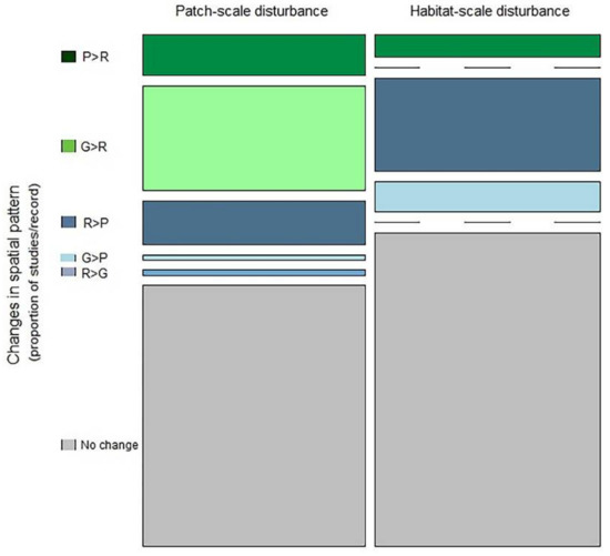
Figure 5.
Mosaic plots of the relative frequency of disturbance-driven changes in the categorical spatial patterns of biodiversity for different scales of disturbance. Bar widths are proportional to the number of studies. The height of each bar segment corresponds the relative frequency of certain type of pattern-change among studies for that scale of disturbance. P > R indicates a shift from patchy to random pattern, G > R indicates a shift from gradient to random, R > P indicates a shift from random to patchy, G > P indicates a shift from gradient to patchy, R > G indicates a shift from random to gradient pattern.
3.5. Causes of Disturbance-Driven Change in Spatial Biodiversity Patterns
Species interactions (22.7% cases), the combined effects of species interactions and dispersal (24.3%), or the combined effects of species interactions and environmental filtering (19.4%) appeared as the key driver underlying the observed changes in the spatial patterns of biodiversity (Figure 6). The unique roles of environmental filtering and dispersal as a driver of changes in spatial biodiversity pattern were identified in about 19.7%, and 13.9% cases, respectively. Interestingly, the role of dispersal was most frequently highlighted in the case of habitat-scale disturbance, while the role of species interactions was frequently highlighted in the case of patch-scale disturbances.
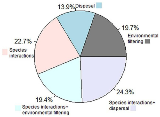
Figure 6.
A pie chart showing the relative frequency of drivers behind changes in the spatial patterns of biodiversity.
4. Discussion
Our analyses demonstrate that habitat disturbances disarrange the spatial patterns of biodiversity, mainly by reducing the overall spatial connectedness and/or by reducing the patch size of species diversity. Moreover, we found that the scale of disturbance can influence the post-disturbance spatial patterns of biodiversity. These results may have important implications, as discussed below, for both spatial ecological theory and applications in grassland/forest management and conservation.
We found an overall declining trend in the spatial patterns of species diversity (Figure 3), which implies that the degree of similarity and the distance, up to which similarity in biodiversity values prevails, may decrease as a result of disturbance. In other words, post-disturbance spatial randomness may increase (Figure 5). This is because disturbances typically disrupt the flow or spatial continuity in habitat abiotic and biotic properties, thereby generating local spatial structures or small patches with distinct vegetation structure [28,48,60]. Such an increase in local spatial structure should lead towards decline in the overall similarity in species diversity for spatially adjacent habitat or towards an overall decline in autocorrelation and spatial range of biodiversity [15]. In fact, recent advances in spatial statistics may allow such local spatial structures to be quantified through orthogonal decomposition of the overall spatial autocorrelation in species or functional diversity into the components of unique positive spatial autocorrelation. This reflects a global spatial structure (variation in local means across the study area), as well as a unique negative spatial autocorrelation reflecting local spatial structure (variation around local means) [15,21,61]. Following this approach, the overall decline in spatial autocorrelation in species diversity can stem from the decline of both positive and negative autocorrelation in a similar fashion, or simply from an increase in negative autocorrelation. Although most of our surveyed studies lumped these two unique components of spatial autocorrelation and derive an overall spatial pattern, Biswas, MacDonald and Chen [15] and Biswas, Mallik, Braithwaite and Wagner [21] analyzed their data by separating unique positive and negative components of spatial autocorrelation. The authors showed that disturbance increases the unique negative autocorrelation in species diversity or functional diversity, while the overall or unique positive components of spatial autocorrelation remained unchanged. Taken together, we suggest that declining spatial autocorrelation and range in the spatial patterns of biodiversity may be attributed to an increase in spatial randomness (noise) or local spatial structures in biodiversity.
Although we did not formally evaluate the effects of disturbance type on the spatial autocorrelation in species or functional diversity, or whether the effects vary among indices of biodiversity, we noticed several interesting trends (Figure A1 and Figure A2). For instance, although spatial autocorrelation generally decreases at different magnitudes for grazing, forest harvesting or other disturbances, there is an increasing trend for burning. This suggests that disturbance type, and possibly disturbance intensity, may play important roles in shaping the post-disturbance spatial autocorrelation in biodiversity. More interestingly, when the effects of disturbance on spatial patterns of several indices of biodiversity were examined, it was often shown that only a small number of indices showed statistically significant result [15,21,34,43]. We also noticed substantial changes in the spatial patterns of species abundance and to some extent in richness and evenness, but not in other indices (Figure A1). That means, disturbances may not impact the spatial patterns of all indices of biodiversity in a similar fashion. It is also possible that disturbance impacts on some indices of biodiversity may not be captured immediately, given that most of our studied literature focused on short-term impacts. Alternatively, it could also mean that possible changes in spatial biodiversity patterns remain undetected, in part, due to lumping of unique positive and unique negative autocorrelation in biodiversity. With raw data, it would be interesting to explore in the future whether the two unique components of spatial autocorrelation in biodiversity respond similarly to disturbances or not. We also call for long-term studies on disturbance-driven changes in the spatial patterns of biodiversity.
Our results indicate that species interaction is the most important driver underlying the observed changes in the spatial patterns of biodiversity, followed by environmental filtering and dispersal (Figure 6). The observed decline in spatial autocorrelation in biodiversity or increasing local spatial structures in biodiversity may, thus, be attributed to species interactions [15,21,45]. It could also mean progressive dominance of generalist species via extirpation of specialist species, leading towards wider scale biotic homogenization [62]. Of course, different processes may create similar patterns, or similar processes may create different patterns, and processes often interact and act in concert [63]. However, most of our surveyed studies inferred the underlying drivers from a pattern, and there existed considerable uncertainly in such an inferential approach [64]. It would be worthwhile to relate the observed spatial biodiversity patterns with process-related variables and identify the causes of changes in the spatial patterns of biodiversity [65,66].
One of the biggest challenge that is apparent from our surveyed literature is to predict the disturbance-driven changes in spatial biodiversity patterns a priori. Most of the studies made such predictions for specific contexts, while our study offers an initial framework to drive a priori hypothesis regarding disturbance-driven changes in the spatial patterns of biodiversity (Figure 1). For instance, if we know the type of habitat spatial heterogeneity (e.g., patchy, gradient or homogeneous), and the type and scale of disturbance (habitat-scale versus patch-scale), then we may draw a priori hypothesis regarding disturbance-driven changes in the spatial patterns of biodiversity. While our framework has received initial support from the reviewed literature (Figure 6), we must caution that more theoretical and empirical studies are needed to verify and refine the framework.
That being said, it is also important to standardize the reporting of methodological details and results. At a minimum level, it is necessary to indicate whether a particular disturbance was applied/occurred at the scale of a patch or habitat, what was the type of pre- and post-disturbance patterns, and what was the type of habitat heterogeneity (e.g., homogeneous, gradient, patch-matrix, mosaic) [26]. Most importantly, reporting on the spatial neighbor information and spatial weighting matrix would greatly help future synthesis to weight different studies differently. This is because the number of neighboring pairs, used to compute spatial autocorrelation, is the true sample size in spatial autocorrelation analysis, and because the design of a spatial weight matrix can greatly influence the results [67].
Space is the final frontier in the ecological understanding and management [25,68], and spatial information is now widely used in conservation and restoration planning [6]. Our results on disturbance-driven spatial disarrangements of biodiversity may imply potential disruption in the continuity of ecological processes and functions across spatial scales [13,53]. Hence, a careful attention towards conserving and promoting spatial biodiversity patterns is necessary [15,21]. While ecosystem managers have already embraced such idea for reserve design [6], the focus lies on the conservation and promotion of spatial patterns at a larger spatial scales, i.e., landscape scale [14]. By contrast, our work emphasizes the importance of conserving and promoting the spatial arrangements of biodiversity at a relatively finer scale. Fuhlendorf, Harrell, Engle, Hamilton, Davis and Leslie Jr. [18] also argued for the conservation and promotion of fine-scale spatial heterogeneity in grassland management. Erdős, Kröel-Dulay, Bátori, Kovács, Németh, Kiss and Tölgyesi [60] also argued for conservation of habitat heterogeneity in forest-grassland mosaics. Interestingly, the idea of conserving and promoting spatial arrangement of biodiversity, be it at a larger or finer spatial scale, is consistent with the concept of conserving and promoting beta diversity [69], or conserving the natural variability [70]. We, thus, suggest that the conservation and promotion of spatial heterogeneity both, at finer and broader scales, may be useful for maintaining ecological processes and functions across spatial scales. That also means that forests and grassland conservation, and management efforts, can be improved by focusing, not only on the average values of local biodiversity, but also on their spatial arrangements.
Several caveats should be taken into account while interpreting our synthesis. First, we were not able to assess the effect of disturbance type, intensity or time since disturbance, due to small number of studies. Several studies found that both spatial autocorrelation and patch size of biodiversity reached their maxima at a moderate intensity of disturbance [38,48,53]. Lumping different intensities of disturbance together may lead to higher within-treatment variability, potentially contributing towards an overall non-significant effects. It would be worth conducting further studies on varying intensities of disturbance on the spatial biodiversity patterns. Second, our study reveals major knowledge gaps in the spatial patterns of functional diversity, underscoring the need for future studies in this aspect. Third, since our data set was not sufficiently large to test all treatment combination levels among our categorical explanatory variables, we separately tested the effects of pre-disturbance spatial patterns and the scale of disturbance on disturbance-driven changes in spatial autocorrelation or spatial range of species or functional diversity. Finally, most of our studies are from forest and grassland, and from species diversity, so our results are best applicable to grazing and forest harvesting disturbances and to species diversity. We call our fellow researchers to come forward and examine how disturbances of different types and intensities might affect the spatial autocorrelation in different indices of biodiversity. While a considerable body of research has been conducted on grasslands and on species diversity, we need more research from other systems, such as forests and savannahs and on functional diversity. Only then can a holistic picture of disturbance-driven changes in the spatial autocorrelation in biodiversity be developed.
Supplementary Materials
The following are available online at https://www.mdpi.com/article/10.3390/d13040167/s1.
Author Contributions
Conceptualization, S.R.B.; methodology, S.R.B. and J.X.; software, S.R.B.; validation, J.X. and H.L.; formal analysis, S.R.B. and J.X.; investigation, J.X. and H.L.; resources, S.R.B.; data curation, J.X. and H.L.; writing—original draft preparation, S.R.B. and J.X.; writing—review and editing, S.R.B., J.X. and H.L.; visualization, S.R.B.; supervision, S.R.B.; project administration, S.R.B.; funding acquisition, S.R.B. All authors have read and agreed to the published version of the manuscript.
Funding
This research was funded by ECNU, grant number 13903-120215-10407. The APC was funded by ECNU-Zijiang Young Professorship Grant (13903-120215-10407).
Data Availability Statement
The data presented in this study are available on supplementary material.
Acknowledgments
We thank all the authors whose works are included in this synthesis. S.R.B. was generously supported by an ECNU- Zijiang Young Professorship Grant (13903-120215-10407).
Conflicts of Interest
The authors declare no conflict of interest. The funders had no role in the design of the study; in the collection, analyses, or interpretation of data; in the writing of the manuscript, or in the decision to publish the results.
Appendix A
Spatial Patterns of Biodiversity and Its Underlying Processes
Spatial patterns of biodiversity can be defined as the degree of similarity or dissimilarity in biodiversity values (mean and median) for spatially adjacent sub-habitats (microhabitats) embedded in a larger habitat. If biodiversity values for spatially adjacent sub-habitats are more similar than the degree of similarity expected by chance, the pattern is called a positively autocorrelated pattern; if the values are less similar than those expected by chance, the pattern is called a negatively autocorrelated pattern; and if no such autocorrelation exits, the pattern is called a neutral/random spatial pattern [6,23,63,71].
Depending on sampling design, the spatial pattern of a variable can be quantified in different ways: When the pattern is assessed based on the actual location of individual organisms, then the pattern is called a point pattern; and when the pattern is assessed in a continuous space based on quantitative values of a variable (i.e., biodiversity index), then the pattern is called a surface or lateral pattern [23]. Spatial range and autocorrelation intensity are the two key properties of a spatial surface pattern. Of which, spatial range indicates the distance up to which similarity in biodiversity values prevail, thereby range indicates the size of a biodiversity patch. The intensity of autocorrelation, on the other hand, indicates the degree of similarity in biodiversity values, thereby autocorrelation intensity indicates the overall spatial connectedness in biodiversity values.
Spatially auto-correlated patterns of biodiversity are typically attributed to several processes, including environmental filtering associated with habitat abiotic conditions and habitat composition (i.e., types of microhabitats embedded in a larger habitat), species interactions associated with species’ abundance and presence, and dispersal restriction associated with the composition and configuration of habitat patches and matrix [26,63,71]. When nearby sub-habitats possess similar abiotic conditions, then the habitat-level population and community patterns can be positively autocorrelated, and vice versa. Neighborhood species interactions can amplify or reduce those spatial patterns, depending on whether a habitat’s environmental conditions are benign or stressful, and how crowded (species abundance) the sub-habitats are. Competition for resources usually thin out crowded individuals in a benign environment, while facilitation promotes positive autocorrelation in a stressful environment; and these effects are expected to be more pronounced in a crowded, rather than sparsely populated conditions. On the other hand, if most of the species are characterized by short-range dispersal and if the dispersal is restricted (e.g., due to the presence of matrix in between sub-habitat patches), then the population and community patterns should be positively autocorrelated, and vice versa.
Appendix B

Figure A1.
Disturbance effects on overall spatial autocorrelation in different indices of species diversity for different types and scales of disturbance. Shown in the figure is mean (solid point) and 95% confidence intervals (solid line) associated with the mean. Statistically significant effects are shown in drak colour, and non-significant effects are shown in grey. Absence of confidence intervals indicates a single study/record (i.e., knowledge gaps). Key points to note that grazing disturbances, either habitat- (41%) or patch-scale (28.76%), reduces the spatial autocorrelation in species abundance substantially (confidence envelops did not overlap zero). Spatial autocorrelation in evenness (25.38%) and richness (86%) also decreased substantially in case of forest harvesting (cf. clear-cutting) and other disturbances, respectively. Although statistically non-significant (confidence interval overlaps zero), burning seems to impact the spatial pattern of species diversity in a unique fashion. For instance, although spatial autocorrelation decreases at different magnitudes for grazing, forest harvesting or other disturbances, it shows an increasing trend for burning.


Figure A2.
Disturbance effects on overall spatial autocorrelation in different indices of functional diversity for different types of disturbance. Shown in the figure is mean (solid point) and 95% confidence intervals (solid line) associated with the mean. Absence of confidence intervals indicates a single study/record (i.e., knowledge gaps).


Figure A3.
Mosaic plots of the relative frequency of disturbance-driven changes in the categories spatial patterns of biodiversity for different types and scales of disturbance. Bar widths are proportional to the number of studies. The height of each bar segment corresponds the relative frequency of certain type of pattern-change among studies for the disturbance type. P > R indicates a shift from patchy to random pattern, G > R indicates a shift from gradient to random, R > P indicates a shift from random to patchy, G > P indicates a shift from gradient to patchy, R > G indicates a shift from random to gradient pattern.

References
- Pereira, H.M.; Leadley, P.W.; Proença, V.; Alkemade, R.; Scharlemann, J.P.W.; Fernandez-Manjarrés, J.F.; Araújo, M.B.; Balvanera, P.; Biggs, R.; Cheung, W.W.L.; et al. Scenarios for Global Biodiversity in the 21st Century. Science 2010, 330, 1496–1501. [Google Scholar] [CrossRef]
- Newbold, T.; Hudson, L.N.; Hill, S.L.L.; Contu, S.; Lysenko, I.; Senior, R.A.; Börger, L.; Bennett, D.J.; Choimes, A.; Collen, B.; et al. Global effects of land use on local terrestrial biodiversity. Nature 2015, 520, 45. [Google Scholar] [CrossRef]
- Sala, O.E.; Chapin, S.F.I.; Armesto, J.J.; Berlow, E.; Bloomfield, J.; Dirzo, R.; Huber-Sanwald, E.; Huenneke, L.F.; Jackson, R.B.; Kinzig, A.; et al. Global Biodiversity Scenarios for the Year 2100. Science 2000, 287, 1770–1774. [Google Scholar] [CrossRef]
- Vellend, M.; Dornelas, M.; Baeten, L.; Beauséjour, R.; Brown, C.D.; De Frenne, P.; Elmendorf, S.C.; Gotelli, N.J.; Moyes, F.; Myers-Smith, I.H.; et al. Estimates of local biodiversity change over time stand up to scrutiny. Ecology 2017, 98, 583–590. [Google Scholar] [CrossRef] [PubMed]
- Legendre, P. Spatial Autocorrelation: Trouble or New Paradigm? Ecology 1993, 74, 1659–1673. [Google Scholar] [CrossRef]
- Fletcher, R.; Fortin, M. Spatial Ecology and Conservation Modeling; Springer: Berlin/Heidelberg, Germany, 2018; p. 523. [Google Scholar] [CrossRef]
- Hovick, T.J.; Elmore, R.D.; Fuhlendorf, S.D.; Engle, D.M.; Hamilton, R.G. Spatial heterogeneity increases diversity and stability in grassland bird communities. Ecol. Appl. 2015, 25, 662–672. [Google Scholar] [CrossRef]
- Turner, M.G. Landscape Ecology: The Effect of Pattern on Process. Annu. Rev. Ecol. Syst. 1989, 20, 171–197. [Google Scholar] [CrossRef]
- Hautier, Y.; Isbell, F.; Borer, E.T.; Seabloom, E.W.; Harpole, W.S.; Lind, E.M.; MacDougall, A.S.; Stevens, C.J.; Adler, P.B.; Alberti, J.; et al. Local loss and spatial homogenization of plant diversity reduce ecosystem multifunctionality. Nat. Ecol. Evol. 2018, 2, 50–56. [Google Scholar] [CrossRef]
- Maestre, F.T.; Escudero, A.; Martinez, I.; Guerrero, C.; Rubio, A. Does spatial pattern matter to ecosystem functioning? Insights from biological soil crusts. Funct. Ecol. 2005, 19, 566–573. [Google Scholar] [CrossRef]
- Rayburn, A.P.; Schupp, E.W. Effects of community- and neighborhood-scale spatial patterns on semi-arid perennial grassland community dynamics. Oecologia 2013, 172, 1137–1145. [Google Scholar] [CrossRef]
- Castillo-Monroy, A.P.; Bowker, M.A.; García-Palacios, P.; Maestre, F.T. Aspects of soil lichen biodiversity and aggregation interact to influence subsurface microbial function. Plant Soil 2015, 386, 303–316. [Google Scholar] [CrossRef]
- Franklin, J.F. Spatial Pattern and Ecosystem Function: Reflections on Current Knowledge and Future Directions. In Ecosystem Function in Heterogeneous Landscapes; Lovett, G.M., Turner, M.G., Jones, C.G., Weathers, K.C., Eds.; Springer: New York, NY, USA, 2005; pp. 427–441. [Google Scholar] [CrossRef]
- Possingham, H.P.; Franklin, J.; Wilson, K.; Regan, T.J. The Roles of Spatial Heterogeneity and Ecological Processes in Conservation Planning. In Ecosystem Function in Heterogeneous Landscapes; Lovett, G.M., Turner, M.G., Jones, C.G., Weathers, K.C., Eds.; Springer: New York, NY, USA, 2005; pp. 389–406. [Google Scholar] [CrossRef]
- Biswas, S.R.; MacDonald, R.; Chen, H. Disturbance increases negative spatial autocorrelation in species diversity. Landsc. Ecol. 2017, 32, 823–834. [Google Scholar] [CrossRef]
- Adler, P.; Raff, D.; Lauenroth, W. The effect of grazing on the spatial heterogeneity of vegetation. Oecologia 2001, 128, 465–479. [Google Scholar] [CrossRef] [PubMed]
- Turner, M.G. Disturbance and landscape dynamics in a changing world. Ecology 2010, 91, 2833–2849. [Google Scholar] [CrossRef]
- Fuhlendorf, S.D.; Harrell, W.C.; Engle, D.M.; Hamilton, R.G.; Davis, C.A.; Leslie, D.M., Jr. Should heterogeneity be the basis for conservation? Grassland bird response to fire and grazing. Ecol. Appl. 2006, 16, 1706–1716. [Google Scholar] [CrossRef]
- Seiferling, I.S.; Proulx, R.; Peres-Neto, P.R.; Fahrig, L.; Messier, C. Measuring Protected-Area Isolation and Correlations of Isolation with Land-Use Intensity and Protection Status. Conserv. Biol. 2012, 26, 610–618. [Google Scholar] [CrossRef]
- Ferrier, S. Mapping spatial pattern in biodiversity for regional conservation planning: Where to from here? Syst. Biol. 2002, 51, 331–363. [Google Scholar] [CrossRef]
- Biswas, S.R.; Mallik, A.U.; Braithwaite, N.T.; Wagner, H.H. A conceptual framework for the spatial analysis of functional trait diversity. Oikos 2016, 125, 192–200. [Google Scholar] [CrossRef]
- Browning, D.M.; Franklin, J.; Archer, S.R.; Gillan, J.K.; Guertin, D.P. Spatial patterns of grassland–shrubland state transitions: A 74-year record on grazed and protected areas. Ecol. Appl. 2014, 24, 1421–1433. [Google Scholar] [CrossRef]
- Fortin, M.-J.; Dale, M.R.T. Spatial Analysis: A Guide for Ecologists; Cambridge University Press: Cambridge, UK, 2005. [Google Scholar] [CrossRef]
- Fraterrigo, J.M.; Rusak, J.A. Disturbance-driven changes in the variability of ecological patterns and processes. Ecol. Lett. 2008, 11, 756–770. [Google Scholar] [CrossRef]
- Levin, S.A. The Problem of Pattern and Scale in Ecology: The Robert H. MacArthur Award Lecture. Ecology 1992, 73, 1943–1967. [Google Scholar] [CrossRef]
- Biswas, S.R.; Wagner, H.H. Landscape contrast: A solution to hidden assumptions in the metacommunity concept? Landsc. Ecol. 2012, 27, 621–631. [Google Scholar] [CrossRef]
- Kim, T.J.; Bullock, B.P.; Stape, J.L. Effects of silvicultural treatments on temporal variations of spatial autocorrelation in Eucalyptus plantations in Brazil. Forest Ecol. Manag. 2015, 358, 90–97. [Google Scholar] [CrossRef]
- Veen, G.F.; Blair, J.M.; Smith, M.D.; Collins, S.L. Influence of grazing and fire frequency on small-scale plant community structure and resource variability in native tallgrass prairie. Oikos 2008, 117, 859–866. [Google Scholar] [CrossRef]
- Benot, M.-L.-L.; Bonis, A.; Rossignol, N.; Mony, C. Spatial patterns in defoliation and the expression of clonal traits in grazed meadows. Botany 2011, 89, 43–54. [Google Scholar] [CrossRef]
- Birkhofer, K.; Scheu, S.; Wise, D.H. Small-Scale Spatial Pattern of Web-Building Spiders (Araneae) in Alfalfa: Relationship to Disturbance from Cutting, Prey Availability, and Intraguild Interactions. Environ. Entomol. 2007, 36, 801–810. [Google Scholar] [CrossRef]
- Camarero, J.J.; Gutiérrez, E.; Fortin, M.-J. Spatial patterns of plant richness across treeline ecotones in the Pyrenees reveal different locations for richness and tree cover boundaries. Glob. Ecol. Biogeogr. 2006, 15, 182–191. [Google Scholar] [CrossRef]
- Chen, J.; Yamamura, Y.; Hori, Y.; Shiyomi, M.; Yasuda, T.; Zhou, H.-K.; Li, Y.-N.; Tang, Y.-H. Small-scale species richness and its spatial variation in an alpine meadow on the Qinghai-Tibet Plateau. Ecol. Res. 2008, 23, 657–663. [Google Scholar] [CrossRef]
- Chen, B.; Yang, G.; Zang, H.; Duan, Q.; Xin, X. Spatial pattern analysis of Leymus chinensis population under different disturbances. Acta Ecol. Sin. 2010, 30, 5868–5874. [Google Scholar]
- Deléglise, C.; Loucougaray, G.; Alard, D. Spatial patterns of species and plant traits in response to 20 years of grazing exclusion in subalpine grassland communities. J. Veg. Sci. 2011, 22, 402–413. [Google Scholar] [CrossRef]
- Díaz, E.R.; Erlandsson, J.; McQuaid, C.D. Detecting spatial heterogeneity in intertidal algal functional groups, grazers and their co-variation among shore levels and sites. J. Exp. Mar. Biol. Ecol. 2011, 409, 123–135. [Google Scholar] [CrossRef]
- Fehmi, J.S.; Bartolome, J.W. Impacts of livestock and burning on the spatial patterns of the grass nassella pulchra (poaceae). Madro 2003, 50, 8–14. [Google Scholar]
- Limb, R.F.; Hovick, T.J.; Norland, J.E.; Volk, J.M. Grassland plant community spatial patterns driven by herbivory intensity. Agric. Ecosyst. Environ. 2018, 257, 113–119. [Google Scholar] [CrossRef]
- Lin, Y.; Hong, M.; Han, G.; Zhao, M.; Bai, Y.; Chang, S.X. Grazing intensity affected spatial patterns of vegetation and soil fertility in a desert steppe. Agric. Ecosyst. Environ. 2010, 138, 282–292. [Google Scholar] [CrossRef]
- Liu, Z.-G.; Li, Z.-Q. Fine-scale spatial patterns of Artemisia frigida population under different grazing intensities. Acta Ecol. Sin. 2004, 24, 227–234. [Google Scholar]
- Liu, J.; Zhang, K. Spatial Pattern and Population Structure of Artemisia ordosica Shrub in a Desert Grassland under Enclosure, Northwest China. Int. J. Environ. Res. Public Health 2018, 15, 946. [Google Scholar] [CrossRef] [PubMed]
- Liu, Z.-G.; Li, Z.-Q.; Nijs, I.; Bogaert, J. Fine-scale spatial pattern of Cleistogenes squarrosa population under different grazing intensities. Acta Pratacult. Sin. 2005, 14, 11–17. [Google Scholar]
- Liu, Z.; Li, Z.; Fu, L.; Dong, M. Small scale spatial pattern of Potentilla acaulis population under different grazing intensities. Chin. J. Appl. Environ. Biol. 2006, 12, 308–312. [Google Scholar]
- Meyers, L.M.; DeKeyser, E.S.; Norland, J.E. Differences in spatial autocorrelation (SAc), plant species richness and diversity, and plant community composition in grazed and ungrazed grasslands along a moisture gradient, North Dakota, USA. Appl. Veg. Sci. 2014, 17, 53–62. [Google Scholar] [CrossRef]
- Montané, F.; Casals, P.; Taull, M.; Lambert, B.; Dale, M. Spatial patterns of shrub cover after different fire disturbances in the Pyrenees. Ann. For. Sci. 2011, 66, 612. [Google Scholar] [CrossRef]
- Moustakas, A. Fire acting as an increasing spatial autocorrelation force: Implications for pattern formation and ecological facilitation. Ecol. Complex. 2015, 21, 142–149. [Google Scholar] [CrossRef]
- Ngoc Le, D.T.; Van Thinh, N.; The Dung, N.; Mitlöhner, R. Effect of Disturbance Regimes on Spatial Patterns of Tree Species in Three Sites in a Tropical Evergreen Forest in Vietnam. Int. J. For. Res. 2016, 2016, 4903749. [Google Scholar] [CrossRef]
- Nolte, S.; Esselink, P.; Smit, C.; Bakker, J.P. Herbivore species and density affect vegetation-structure patchiness in salt marshes. Agric. Ecosyst. Environ. 2014, 185, 41–47. [Google Scholar] [CrossRef]
- Nunes, P.A.d.A.; Bredemeier, C.; Bremm, C.; Caetano, L.A.M.; de Almeida, G.M.; de Souza Filho, W.; Anghinoni, I.; Carvalho, P.C.d.F. Grazing intensity determines pasture spatial heterogeneity and productivity in an integrated crop-livestock system. Grassl. Sci. 2019, 65, 49–59. [Google Scholar] [CrossRef]
- Olofsson, J.; de Mazancourt, C.; Crawley, M.J. Spatial heterogeneity and plant species richness at different spatial scales under rabbit grazing. Oecologia 2008, 156, 825–834. [Google Scholar] [CrossRef]
- Rietkerk, M.; Ketner, P.; Burger, J.; Hoorens, B.; Olff, H. Multiscale soil and vegetation patchiness along a gradient of herbivore impact in a semi-arid grazing system in West Africa. Plant Ecol. 2000, 148, 207–224. [Google Scholar] [CrossRef]
- Schaefer, J.A. Spatial patterns in taiga plant communities following fire. Can. J. Bot. 1993, 71, 1568–1573. [Google Scholar] [CrossRef]
- Yu, H.; Yang, X.-H.; Ci, L.-J. Variations of spatial pattern in fire-mediated mongolian pine forest, Hulun Buir sand region, Innner Mongolia, China. Chin. J. Plant Ecol. 2009, 33, 71–80. [Google Scholar]
- Yuan, F.; Wu, J.; Li, A.; Rowe, H.; Bai, Y.; Huang, J.; Han, X. Spatial patterns of soil nutrients, plant diversity, and aboveground biomass in the Inner Mongolia grassland: Before and after a biodiversity removal experiment. Landsc. Ecol. 2015, 30, 1737–1750. [Google Scholar] [CrossRef]
- Gibson, D.J. The Relationship of Sheep Grazing and Soil Heterogeneity to Plant Spatial Patterns in Dune Grassland. J. Ecol. 1988, 76, 233–252. [Google Scholar] [CrossRef]
- Vellend, M.; Baeten, L.; Myers-Smith, I.H.; Elmendorf, S.C.; Beauséjour, R.; Brown, C.D.; De Frenne, P.; Verheyen, K.; Wipf, S. Global meta-analysis reveals no net change in local-scale plant biodiversity over time. Proc. Natl. Acad. Sci. USA 2013, 110, 19456–19459. [Google Scholar] [CrossRef]
- Hedges, L.V.; Gurevitch, J.; Curtis, P.S. The meta-analysis of response ratios in experimental ecology. Ecology 1999, 80, 1150–1156. [Google Scholar] [CrossRef]
- Crowder, D.W.; Northfield, T.D.; Gomulkiewicz, R.; Snyder, W.E. Conserving and promoting evenness: Organic farming and fire-based wildland management as case studies. Ecology 2012, 93, 2001–2007. [Google Scholar] [CrossRef]
- Adler, P.B.; Smull, D.; Beard, K.H.; Choi, R.T.; Furniss, T.; Kulmatiski, A.; Meiners, J.M.; Tredennick, A.T.; Veblen, K.E. Competition and coexistence in plant communities: Intraspecific competition is stronger than interspecific competition. Ecol. Lett. 2018, 21, 1319–1329. [Google Scholar] [CrossRef] [PubMed]
- Murphy, G.E.P.; Romanuk, T.N. A Meta-Analysis of Community Response Predictability to Anthropogenic Disturbances. Am. Nat. 2012, 180, 316–327. [Google Scholar] [CrossRef]
- Erdős, L.; Kröel-Dulay, G.; Bátori, Z.; Kovács, B.; Németh, C.; Kiss, P.J.; Tölgyesi, C. Habitat heterogeneity as a key to high conservation value in forest-grassland mosaics. Biol. Conserv. 2018, 226, 72–80. [Google Scholar] [CrossRef]
- Dray, S. A New Perspective about Moran’s Coefficient: Spatial Autocorrelation as a Linear Regression Problem. Geogr. Anal. 2011, 43, 127–141. [Google Scholar] [CrossRef]
- Abadie, J.-C.; Machon, N.; Muratet, A.; Porcher, E. Landscape disturbance causes small-scale functional homogenization, but limited taxonomic homogenization, in plant communities. J. Ecol. 2011, 99, 1134–1142. [Google Scholar] [CrossRef]
- Legendre, P.; Fortin, M.J. Spatial pattern and ecological analysis. Vegetatio 1989, 80, 107–138. [Google Scholar] [CrossRef]
- McIntire, E.J.B.; Fajardo, A. Beyond description: The active and effective way to infer processes from spatial patterns. Ecology 2009, 90, 46–56. [Google Scholar] [CrossRef] [PubMed]
- Biswas, S.R.; Wagner, H.H. Spatial structure in invasive Alliaria petiolata reflects restricted seed dispersal. Biol. Invasions 2015, 17, 3211–3223. [Google Scholar] [CrossRef]
- Cottenie, K. Integrating environmental and spatial processes in ecological community dynamics. Ecol. Lett. 2005, 8, 1175–1182. [Google Scholar] [CrossRef]
- Stakhovych, S.; Bijmolt, T.H.A. Specification of spatial models: A simulation study on weights matrices. Pap. Reg. Sci. 2009, 88, 389–408. [Google Scholar] [CrossRef]
- Kareiva, P. Special Feature: Space: The Final Frontier for Ecological Theory. Ecology 1994, 75, 1. [Google Scholar] [CrossRef]
- Socolar, J.B.; Gilroy, J.J.; Kunin, W.E.; Edwards, D.P. How Should Beta-Diversity Inform Biodiversity Conservation? Trends Ecol. Evol. 2016, 31, 67–80. [Google Scholar] [CrossRef] [PubMed]
- Keane, R.E.; Hessburg, P.F.; Landres, P.B.; Swanson, F.J. The use of historical range and variability (HRV) in landscape management. For. Ecol. Manag. 2009, 258, 1025–1037. [Google Scholar] [CrossRef]
- Wagner, H.H.; Fortin, M.-J. Spatial analysis of landscapes: Concepts and statistics. Ecology 2005, 86, 1975–1987. [Google Scholar] [CrossRef]


Publisher’s Note: MDPI stays neutral with regard to jurisdictional claims in published maps and institutional affiliations. |
© 2021 by the authors. Licensee MDPI, Basel, Switzerland. This article is an open access article distributed under the terms and conditions of the Creative Commons Attribution (CC BY) license (https://creativecommons.org/licenses/by/4.0/).