Article

Recognition and Characterization of Forest Plant Communities through Remote-Sensing NDVI Time Series

by
Simone Pesaresi
1,
Adriano Mancini
2 and
Simona Casavecchia
1,*
1
Department of Agricultural, Food, and Environmental Sciences, D3A, Università Politecnica delle Marche, Via Brecce Bianche 12, 60131 Ancona, Italy
2
Department of Information Engineering, DII, Università Politecnica delle Marche, Via Brecce Bianche 12, 60131 Ancona, Italy
*
Author to whom correspondence should be addressed.
Diversity 2020, 12(8), 313; https://doi.org/10.3390/d12080313
Submission received: 1 July 2020 / Revised: 5 August 2020 / Accepted: 12 August 2020 / Published: 14 August 2020
(This article belongs to the Special Issue Plant Community Ecology: From Theory to Practice)

Abstract

:
Phytosociology is a reference method to classify vegetation that relies on field data. Its classification in hierarchical vegetation units, from plant associations to class level, hierarchically reflects the floristic similarity between different sites on different spatial scales. The development of remotely sensed multispectral platforms as satellites enormously contributes to the detection and mapping of vegetation on all scales. However, the integration between phytosociology and remotely sensed data is rather difficult and little practiced despite being a goal for the modern science of vegetation. In this study, we demonstrate how normalized difference vegetation index (NDVI) time series with functional principal component analysis (FPCA) could support the analyses of phytosociologists. The approach supports the recognition and characterization of forest plant communities identified on the ground by the phytosociological approach by using NDVI time series that encode phenological behaviors. The methodology was evaluated in two study areas of central Italy, and it could characterize and discriminate six different forest plant associations that have similar dominant tree species but distinct specific composition: three dominated by black hornbeam (Ostrya carpinifolia) and three dominated by holm oak (Quercus ilex). The methodology was also able to optimize the ground data collection of unexplored areas (from a phytosociological point of view) by using a phenoclustering approach. The obtained results confirmed that by using remote sensing, it is possible to separate and distinguish plant communities in an objective/instrumental way, thus overcoming the subjectivity intrinsic to the phytosociological method. In particular, FPCA functional components (NDVI seasonalities) were significantly correlated with vegetation abundance data variation (Mantel r = 0.76, p < 0.001).

Graphical Abstract

1. Introduction

The recognition and characterization of plant communities can be achieved with various approaches. Starting from the 20th century, one of the most followed methods, at least in Europe, was that proposed by the school of Zurig-Montpellier [1], which is known as phytosociology. The cornerstones of phytosociology, as explained by its founder [1] are as follows: (1) the study of plant communities, their composition, and their ecological role through the recognition of a pool of “characteristic” species in order to classify vegetation in discrete units called “plant associations”; (2) the analysis of the relationships between plant communities and the environmental conditions (synecology); (3) the study of the evolution of plant communities from their rise to their decline (Syngenetics); (4) the study of the distribution range of plant communities (Synchorology); (5) the classification and ordination of plant communities into a hierarchical frame (Synsystematics). Indeed, the method provides that plant associations, compared with each other, are brought together in hierarchical levels from which hierarchical classification derives, similar to that used for general systematics [2,3]. According to present-day developments [4], an association is defined as “a system of plants having a floristic composition that is statistically repetitive; it has a range of different features, such as the structure, the ecological value (significant for different environmental parameters), and the quality of the dynamic and catenal relationships that it has with other communities”. Moreover, it stands out for “a characteristic specific complex, consisting of the preferring plants which are particularly linked to it in statistical terms and that are biogeographically and ecologically differential compared to similar synvicariant or geosynvicariant associations’’. Therefore, phytosociology is a scientific discipline with high ecological and biogeographic connotation; indeed, it is based on three levels of analysis that can be considered stages of development reached over time: (1) the floristic–ecological approach, based on the recognition of plant associations; (2) the synphytosociological approach, based on the study of time–dynamical relationships among associations in order to identify dynamic vegetation series (integrated phytosociology); and (3) geosynphytosocology, also known as landscape phytosociology, which, through the knowledge of the spatial distribution of different vegetation series, recognizes homogeneous landscape units in terms of bioclimatic and geographic features [5].
One of the applications of the phytosociological method is the mapping of vegetation by the production of phytosociological maps, the mapping of vegetation series (synphytosociological map), and the mapping of landscape units (geosynphytosociological maps). These maps are full of ecological information, as they can be considered “integrated maps”; indeed, vegetation communities are correlated to environmental data such as bioclimatic features, topographic conditions, lithology, and land use. The widespread use of this approach in the botanical scientific community has meant that a large part of the world’s vegetation has been studied and classified using a standard and shared methodology [6] with the production of a large amount of data collected in various databases of more or less easy access (i.e., [7,8]).
With the development of satellite technology, remote vegetation detection has represented a methodological evolution of great application interest. However, the integration between phytosociology and remote sensing still remains difficult [9], so much so that the “combined” approach that involves the use of remote-sensing technologies associated with field surveys still remains a target to be satisfied [4,6,10]. The greatest difficulties encountered are to identify a correspondence between remote-sensing products and plant communities that sometimes differ from each other by a few species (diagnostic species) that are difficult to be captured by sensors [11]. As an example, in the study of forests based solely on remote-sensing data, one of the main difficulties is represented by the recognition of typologies with similar dominant tree species composition, which prevalently differ by their understory vegetation [12].
This difficulty is even more evident in transition areas between two or more bioclimatic typologies, i.e., between the Mediterranean and the temperate bioclimate, where it is difficult to separate communities with many species in common. To do this requires a great deal of detailed analysis, especially based on direct observations and sampling on the field [13,14,15] and from remote systems. In fact, studies that can be found in the literature concerning the spatialization of plant communities using remote systems concern very large surfaces, such as discrimination between biomes or between physionomic formations [16,17,18,19]. For the purposes of environmental management and the implementation of territorial policies, the discrimination of small-scale plant communities is essential, and the required accuracy is very high. In particular, the implementation of conservation measures and the subsequent verification envisaged by the European biodiversity conservation policy (Habitats Directive) require the production of detailed maps in which various plant communities recognized as habitats of community interest are precisely mapped in order to monitor their increase/contraction in terms of surface over time.
A key aspect that can help detect the composition of plant communities and their spatial patterns is the use of remotely sensed (multispectral or hyperspectral) data that capture the “greenness” dynamics of a landscape (often quantified in vegetation indices such as the normalized difference vegetation index (NDVI)) [20,21,22,23,24,25]. The use of remotely sensed data and time series is becoming a core aspect of land surface phenology (LSP) [26]. LSP could be defined as the seasonal/annual pattern of (phenological) variation in vegetated land surfaces detected by using remote sensing. In this context, today, it is possible to distinguish and map vegetation types and/or plant communities [19,27,28] in order to monitor human disturbance on wild ecosystems and the effects of climate changes on plant phenology [29], plan management strategies [30], or even to develop phenoregions [31]. The phenological behavior of a species community may depend on environmental characteristics of the site because of the adaptability that plants have toward abiotic factors such as temperature, solar irradiation, water availability, and competition with other animal and plant species [32,33]. The same species can have different phenological behavior in different bioclimatic and geographic contexts. This could lead to an association with species having the same environmental needs that can share similar phenological behavior. Particularly important is the length of the vegetative period, which means the time in which the plant can complete its vegetative and reproductive cycle [22].
Recently, the use of remotely sensed NDVI time series combined with functional data analysis opened new ways to understand phenology, supporting phytosociologists. It is possible to integrate phytosociological data with remotely sensed data to find a relationship with syntaxonomic units of high detail that are plant associations and habitats, as in our previous work [10]. In this work, we show that plant communities are distinguished by floristic composition and phenological behavior, and NDVI time series processed with a functional approach are helpful to improve habitat mapping.
In this work, we extend the methodology to another study area that has similar plant communities (with similar dominant tree species). We were also interested in testing if the methodology could recognize and characterize different forest plant communities identified by the phytosociological approach for both study areas. We focused on the characterization of different types of holm oak (Quercus ilex) and black hornbeam (Ostrya carpinifolia) woods that develop in different bioclimatic and geographical conditions in order to verify the existence of different phenological behavior useful to discriminate different communities of plants. Our goal was to demonstrate that holm oak woods that extend, respectively, along the sides of a coastal mountain and along a mountain of the Apennine ridge, although traditionally attributed to the same plant association on the basis of phytosociological interpretation, actually have different characteristics (traits) in terms of floristic composition and phenological behavior. The same objective was also applied to forest formations of black hornbeam that are found in the same geographical areas.
This work is structured as it follows. Section 2 presents the material and methods focused on the NDVI time series, functional analysis, dataset, and study sites. Section 3 presents the main results derived from functional and cluster analysis, and we discuss the impact of our methodology for phytosociological analysis and mapping in Section 4. Section 5 outlines the conclusion and future works.

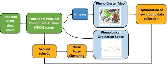
2. Materials and Methods
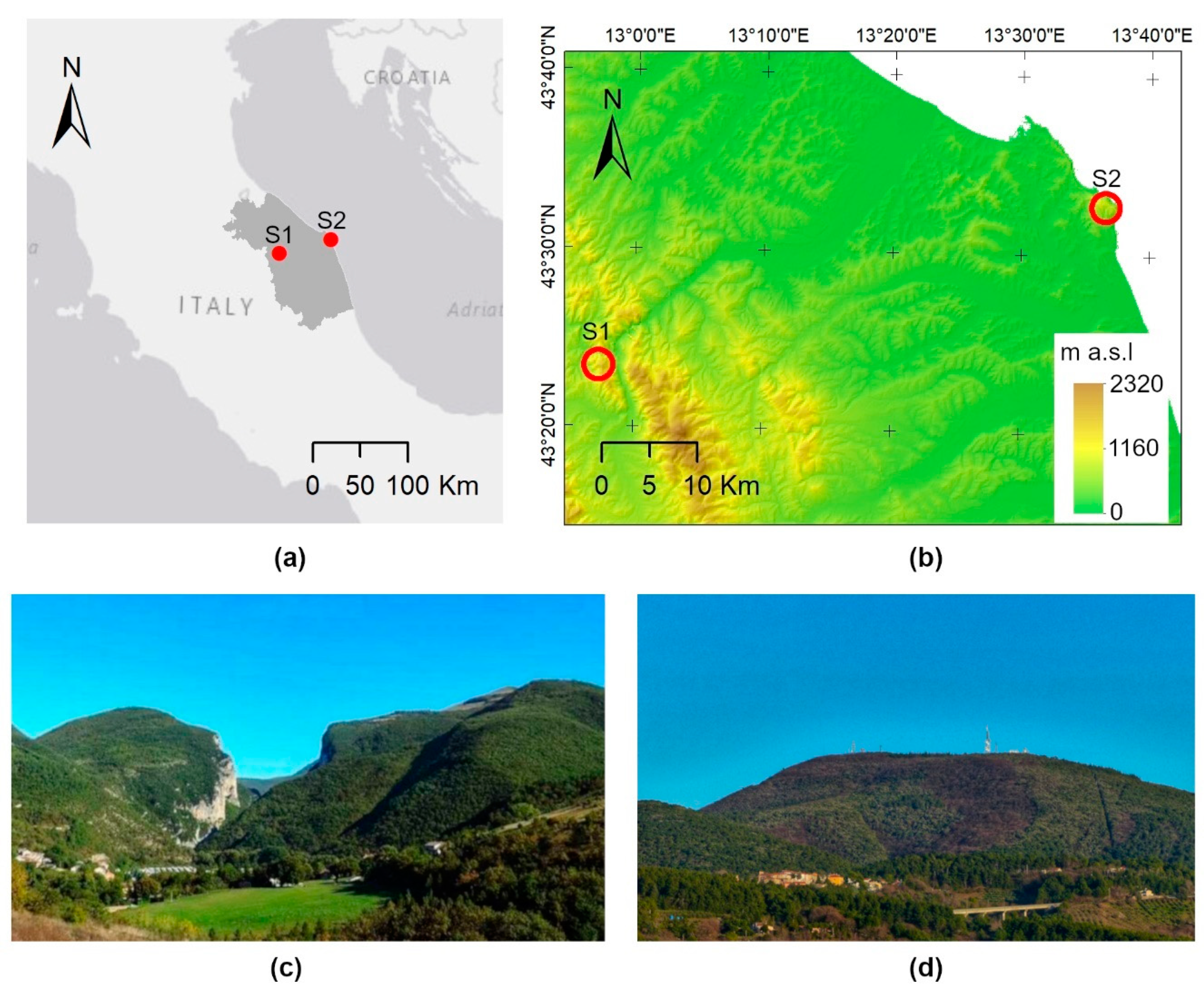
In this section, we introduce the study sites, providing details regarding plant communities and aspects related to their location. Then, we summarize how NDVI time series are generated from satellite images and processed by using functional principal component analysis (FPCA). In the remaining part, we detail phytosociological data collection and ground data classification to detect and recognize plant communities. Figure 1 shows the graphical representation of the methodology we applied to the study site (see Figure 2).

2.1. Study Area

Holm oak woods represent a very common forest typology in Mediterranean areas. In Italy, they are located mainly in coastal areas, but in strong-slope conditions along limestone mountains, they could also be found in temperate (sub-Mediterranean) locations close to the Apennine mountains. Holm oak associations described for central Italy are different in their floristic composition [34]. In the study areas of this work, we found two main holm oak associations: the first (Cyclamino hederifoliiQuercetum ilicis) is defined as thermophilic, as it is rich in evergreen Mediterranean species and widespread in warmer coastal areas; the second (Cephalanthero longifoliaeQuercetum ilicis) is considered mesophilic, as there are deciduous species in its composition, both in the tree layer and in the understory, where species more typical of temperate woods occur [35]. However, for the internal Apennine areas, no associations were described, but the same communities are used despite the floristic composition clearly being different.
Black hornbeam forests occupy large areas in the Italian peninsula, where they occur on the slopes of hills and mountains from coastal and subcoastal areas at altitudes between 100 and 400–500 a.s.l., approximately up to internal mountain areas at altitudes that can exceed 800–900 m a.s.l. [36]. For the Marche region, on limestone rocks, the main described plant associations are Asparago acutifoliiOstryetum carpinifoliae and Scutellario columnaeOstryetum carpinifoliae. The first association is considered a thermophilous community typical of the sub-Mediterranean bioclimate because, in the understory, typical species of Mediterranean forests occur, and, in the tree layer, holm oak is often present. On the other hand, the second association refers to mesophilic temperate woods with more typically temperate species; they often interpenetrate with beech woods that, in central Italy, represent the most mesophilic and typically mountainous forest typology [35,37].
The first area of interest for this study is represented by the limestone sector of Mount Conero (43°33′00′’ N, 13°36′00′’ E), which is localized in the coastal area of central Marche, reaching an altitude of 572 m a.s.l. It is part of the Natura 2000 network, as it is included in a special area of conservation (SAC) Monte Conero (code IT5320007). The mean annual precipitation is 710 mm, while the mean annual temperature is 14.9 °C. According to the bioclimatic classification of Rivas-Martinez et al. [38], the area belongs to the temperate macrobioclimate with a strong level of sub-Mediterraneity because of strong summer aridity [39]. The lithological substrate on which the investigated forests develop is made up of limestone, which is referable to the ‘majolica’ and ‘scaglia bianca’ formations. In this context, we found the presence of two holm oak associations and one association of black hornbeam according to the Marche SIT-REM project [40].
The second study area, Mount Valmontagnana (43°23′23′′ N, 12°57′36′′ E), is located in the mountainous area of the central Apennines (on Marche’s border), and it reaches the altitude of 935 m a.s.l. It is part of the Gola di Frasassi (also known as the Gorge of Frasassi) special area of conservation (SAC) (code IT5320003). The average annual precipitation is 1115 mm, while the average annual temperature is 12.7 °C. According to the bioclimatic classification of Rivas-Martinez et al. [38], the area belongs to the temperate macrobioclimate with a weak sub-Mediterranean level, which indicates low summer aridity [39]. The mountain is mainly characterized by calcareous lithotypes of the Umbria–Marche formation, and the studied forests are located on ‘calcare massiccio’, ‘majolica’, and ‘scaglia bianca’ formations. In this area, we found two different typologies of holm oak woods and two of black hornbeam [40]. Figure 2 shows the localization of the study area of Mount Valmontagnana (Figure 2c) and Mount Conero (Figure 2d) in the context of Marche’s region.

2.2. Remotely Sensed NDVI Times Series

In this work, we focused on NDVI without a loss of generality of the proposed methodology. We used NDVI to establish a baseline to validate the idea behind this work—that is, to recognize and characterize forest plant communities through remote-sensing time series. All Landsat 8 Level-2 images available for the period of April 2013–April 2019 were collected for the two studies. We considered a scene as valid in case of cloud coverage in the areas of interest below 25%. In this study, 54 images for the Mount Valmontagnana area and 91 for the Mount Conero site were selected. We preprocessed images to mask the clouds and normalize the topographic effect [41], and we calculated the NDVI (with the R RStoolbox package [42]). NDVI profiles over several years can be averaged to establish an annual mean phenological profile of vegetation [43]. Then, NDVI data were chronologically ordered according to the day of year (DoY), and outliers were identified and removed by the clean.ts() function of the “forecast” R package [44,45]. DoY NDVI values were aggregated to biweekly mean values to obtain dense and regular pixel-based NDVI times series. The biweekly pixel-based NDVI series were smoothed by a generalized additive model (GAM) [46], obtaining a cubic spline representation of NDVI time series.

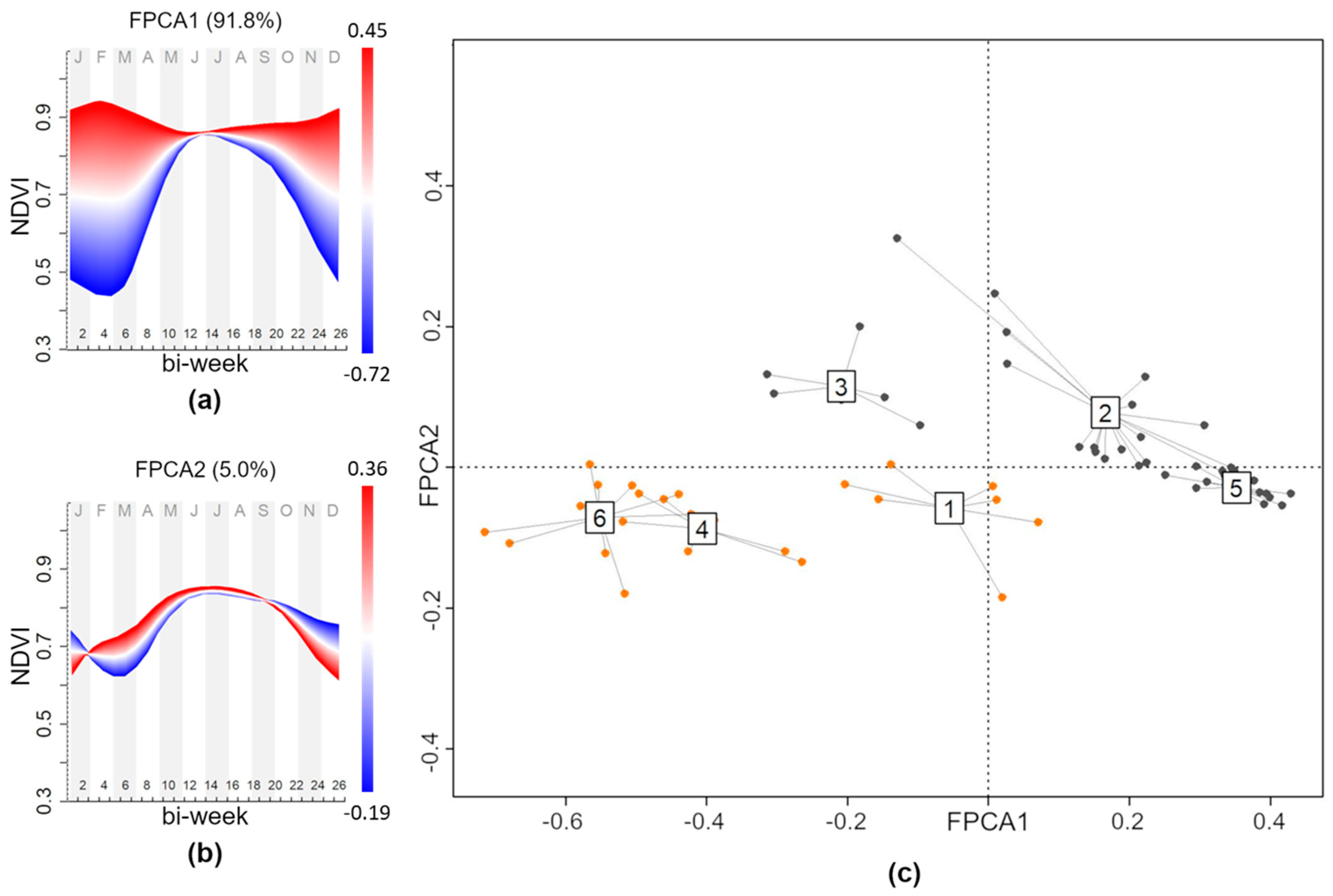
2.3. NDVI Seasonality: Functional Principal Component Analysis of NDVI Time Series

Functional principal component analysis (FPCA) is a tool of functional data analysis that, as in PCA, compresses information on an orthonormal basis. FPCA, if compared with PCA, preserves the temporal structure of the data [47]. For this reason, FPCA is more appropriate for time-series analysis than PCA. FPCA extracts functional principal components from the functional data space (e.g., NDVI time series), describing the temporal structure of timed data (NDVI seasonalities) [48]. FPCA, analogously to the PCA, provides eigenvalues that account for the variation explained by each component and the FPCA scores that quantify the similarity between functions (NDVI time series). FPCA scores are a core aspect of this study, as they could be used in subsequent analysis (e.g., correlation analysis, functional data clustering [49]). In an ordered reduced space (here, a phenological space), the functions (here, the NDVI time series) could be plotted supporting experts in ecological interpretation [10,50].
FPCA was used for two main objectives: (1) to “guide” (steer) phytosociological sampling on the ground in the Valmontagnana area (phytosociologically unexplored over the 2013–2019 period—see Section 2.4); and (2) to identify remotely sensed time-series differences in the locations of the phytosociological surveys, evaluating the relationships of different black hornbeam and holm oak forest plant community compositions inside the two study areas (see Section 2.6). This analysis was also carried out considering Mounts Valmontagnana and Conero as a whole. FPCA was performed using the “fdapace” R package [51].

2.4. Phytosociological Data Collection

2.4.1. Data-Driven Ground Data Collection

The collection of ground data in the context of the recognition and characterization of forest plant communities could be a challenging task considering that regions could be wide in terms of area and, in some cases (i.e., Mount Valmontagnana or Conero of this study), they could be remote with limited access. For this reason, the rational planning of ground-survey campaigns should be supported/driven by a set of information that could be a priori knowledge of the area, such as phytosociological maps. Problems arise in the case of updated maps not being reported [9]. This potential issue could be strongly mitigated if remotely sensed data are used to drive the decision to select areas with interesting and unexpected behaviors.
Satellites could be used to steer expert decisions, and the use of NDVI time series is a valid tool to be adopted. Starting from the time series, it is possible to derive areas that share over time similar (phenological) behavior (e.g., phenocluster or phenoclasses [30]). The identification of these areas is possible if the FPCA scores of NDVI time series are features that are classified by using an unsupervised approach that could be summarized as functional data clustering (FDC) [49].
The key aspect of our approach is the use of FPCA scores derived from FPCA that can describe the dynamics of the NDVI time series. The output of this process is a thematic (phenocluster) map that could be used to plan a ground survey. This map is also able to show areas with unexpected behavior if compared with existing phytosociological data.

2.4.2. Ground Dataset

The dataset of this study was composed by two subsets restricting focus to forest plant communities dominated by holm oak and black hornbeam. The main aim was to compare two different areas (coastal and Apennine) that share similar forest plant communities. The first subset, namely, Mount Conero, was derived from our previous study [10]. This area was previously also studied in detail from a phytosociological point of view [35,52]. The second subset refers to the area of Mount Valmontagnana. This area is partially unexplored from a phytosociological point of view, and there was a lack of updated phytosociological relevés in the 2013–2019 period. Previous phytosociological maps [40] were used to mask forest plant communities that were not dominated by holm oak and black hornbeam (Figure 3a).
For this reason, we designed the selection of phytosociological relevé locations by using FDC analysis starting from the NDVI time series. FDC is based on an unsupervised clustering approach. The FPCA component scores of a pixel-based NDVI time series represent the set of features. In our case, we used k-means, but it is of course possible to also use other approaches to perform clusterization.
We limited the number of clusters to two. In the case of Mount Conero, considering the availability of updated and high-resolution phytosociological relevés and phytosociological data, we directly selected phytosociological relevés from both existing maps and ground campaigns. Table 1 summarizes the details of the dataset for both the Mount Conero and Valmontagnana areas. The phytosociological relevés were proportional to the area of each cluster.

2.5. Plant Communities: Ground Data Classification

To identify forest plant communities of the two study areas, noise fuzzy clustering (NFC) was applied to the Hellinger-transformed vegetation abundance data [53,54]. Noise fuzzy clustering can classify phytosociological relevés (cluster) and at the same time identify anomalous (outlier) ones. The fuzzyness coefficient and distance from the noise class were set to 1.15 and 0.8, respectively (in accordance with those suggested by De Caceres et al. [53]). The optimal number of clusters (forest plant communities) was identified according to the minimal value of the normalized partition entropy index (PEN) obtained by repeating noise fuzzy clustering from 2 to 10 groups. The crisp final classification of the phytosociological relevés was obtained according to their maximal fuzzy membership values across clusters [53]. Indicator species analysis was performed to identify the indicator species of the clusters (phi coefficient > 0.4, p-value < 0.05) [55].

2.6. NDVI Seasonality and Forest Plant Community Relationships

Starting from the set of preprocessed images, we extracted the NDVI time series for each location that has a phytosociological relevé. We derived 64 NDVI time series (24 for the Mount Valmontagnana area and 40 for the Mount Conero one). These time series were analyzed by FPCA. Correlation between NDVI seasonality (quantified by pairwise Euclidean distances among plots on the basis of FPCA scores) and vegetation abundance variation (quantified by pairwise Hellinger distance among plots) was quantified and tested with the Mantel test [56]. Then, the phytosociological relevés were plotted in the functional ordered reduced space (reduced NDVI phenological space) according to their FPCA scores. To determine the statistical differences of the plant communities in phenological behavior (FPCA space), we conducted permutational multivariate analyses of variance (PERMANOVA) [57] using the Adonis function in the vegan package (nperm = 9999, α = 0.05) [58]. We used pairwise.adonis (nperm = 9999, with Holm correction for p-values) [59] to test for significant differences between pairs of plant communities. Plant communities (clusters) were superimposed on the functional ordered reduced space to show their relationship with distinct NDVI seasonality recognized by FPCA. Lastly, FPCA scores were used to fit the mean annual NDVI profile of the plant communities. Figure 1 shows the overall adopted methodology.

3. Results

3.1. Phytosociological Data Collection

Figure 3 shows the spatiotemporal patterns of the two phenoclusters of the Mount Valmontagnana area obtained with FDC (k-means of the two first FPCA component scores that accounted for 96.7% of the total variation) of pixel-based Landsat 8 NDVI time series. A ground-survey campaign was carried out showing the total correspondence between the two phenoclusters and the two types of forest (black hornbeam and holm oak woods) in the 24 phytosociological relevés. The 17 phytosociological relevés of the first phenocluster (green in Figure 3) were woods dominated by black hornbeam, while the 7 of the second phenocluster (red in Figure 3) were woods dominated by holm oak. Phytosociological sampling guided by the phenoclusters allowed for detecting unexpected holm oak woods (northwestern part of the red phenocluster in Figure 3c) whose occurrence was not revealed or spatially explicated in the last produced phytosociological map ([40], Figure 3a).

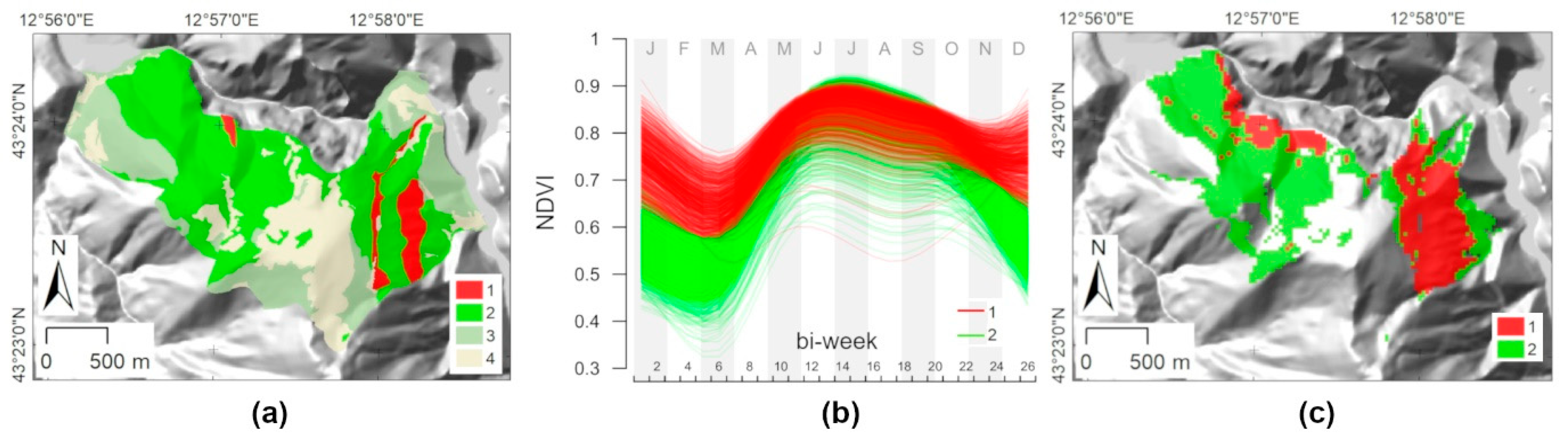
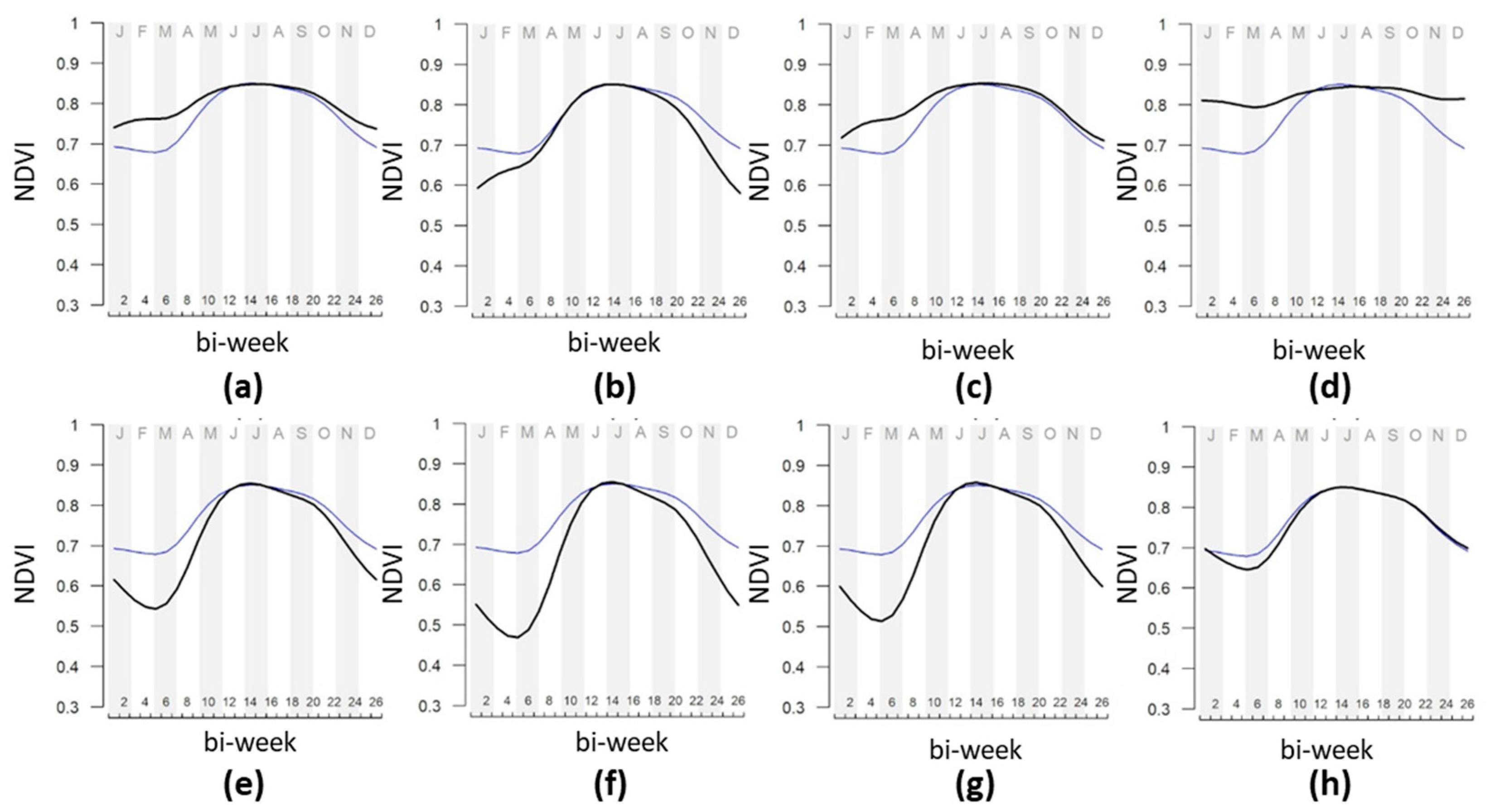
3.2. Forest Plant Communities and NDVI Seasonality Relationships

The NFC, according to PEN values, was able to identify six forest typologies (clusters) with distinct floristic composition. Three forest plant communities are dominated by black hornbeam (Clusters 4 and 6 for the Mount Valmontagnana area, and Cluster 3 for the Mount Conero area), while three are dominated by holm oak (Cluster 1 for the Mount Valmontagnana area, and Clusters 2 and 5 for the Mount Conero area). Table A1 summarizes the average floristic composition of the six forest plant communities and their indicator species.
FPCA of the NDVI time series of the 64 phytosociological relevés identified 5 functional principal components (NDVI seasonalities). The first two FPCA components accounted for 96.8% of total NDVI variation (FPCA1: 91.8%; FPCA2: 5.0%). FPCA functional components (NDVI seasonalities) were significantly correlated with vegetation abundance data variation (Mantel r = 0.76, p < 0.001). All plant communities showed significant differences in NDVI seasonalities (PERMANOVA pseudo-F = 118.57 p-values = 0.0001; pairwise PERMANOVA adjusted p-values reported in Table A2). Variation in vegetation composition corresponded to a different remote-sensing NDVI temporal profile. FPCA1 and FPCA2 functional components were used to define the reduced phenological ordination space of the phytosociological relevés locations. Cluster analysis results and a spider plot (Figure 4c) show and support the interpretation of a distinct forest plant community phenology. FPCA1 (Figure 4a) accounts for autumn–winter NDVI variation. This component could separate the occurrence of black hornbeam forests (Clusters 3, 4, and 6) from those dominated by holm oak (Clusters 1, 2, 5), and corresponded to a deciduousness–evergreens gradient. FPCA2 (Figure 4b) mapped the shifting time of NDVI changes in the spring and late-autumn periods. This functional component mainly discriminated the localities of 1–3 clusters that have quite a balanced composition of deciduous and evergreen species, which are located in the central part of FPCA1. This component separated the Mount Valmontagnana and Mount Conero areas. Figure 5 shows the mean annual NDVI time profile of the six forest plant communities (clusters) and those of the two study areas. Figure 5 shows how clusters exhibited different phenological behaviors that are a meaningful source of information for phytosociologists, as discussed in the next section.

4. Discussion

4.1. General Discussion

The methodology presented in this work was evaluated on two different test areas with similar plant communities to establish a relationship between forest plant communities and phenological behavior, which is detectable using remotely sensed data. The approach proposed here relies on functional principal component analysis applied to NDVI time series from satellite data (i.e., Landsat 8). The obtained results and the high values of the Mantel test (r = 0.76), as presented in Section 3, showed high correlation between remotely sensed NDVI time series (FPCA scores) and the specific composition of forest plant communities (plant β-diversity). The Mantel r here was obtained using NDVI time series; therefore, only a limited spectral band was in agreement (and even higher) with those obtained with a combination of multispectral and multitemporal remotely sensed variables [25,60]. This result, also considering the output of the PERMANOVA test, reinforces the link between variation in plant community species composition (ground data) and vegetation phenology (remote-sensing detected).
Functional data analysis, specifically FPCA, is a powerful tool to process NDVI times series. This method can extract the (few orthogonal) main NDVI time-series variations, preserving the temporal structure of data. This method allows for the characterization and the discrimination of forest communities of the same physiognomic category, even when floristic composition is distinguished by few species (e.g., nemoral diagnostic species; see Table A1).
The representation of clusters on reduced phenological space ordination (forest plant communities), as shown in Figure 4c, facilitates the interpretation of forest plant community ecology and phenology (similarly to Brooks et al. [61]), integrating sensor-based and field monitoring data (e.g., [10,50]). A comprehensive method that translates remote-sensing data into vegetation units that are defined a priori and based on species composition, such as phytosociological units, is desired [11]. It also opens the way to understand diversity that is attributable, for example, to the floristic component.
The proposed methodology also simplifies the selection of remotely sensed data (i.e., satellite scenes) to be used. The method proposed here considered all available valid images (see Section 2.2). There was no need to select the best reference scene over the reference period. Starting from all images, we generated the time series. This aspect made our approach less sensitive to the selection of the best image to be used (as in [25,62]), eliminating any qualitative selection process. Then, time-series data were interpolated, preserving dynamics and reducing the noise by GAM.
The methodology proposed here was also used to select the most interesting areas to plan ground surveys. This represents a sort of scouting and planning tool supporting the planning of ground data collection, which is an expensive and complex task. Unsupervised phenoclustering from FPCA scores simplified the identification of areas to check in situ to build up the dataset (phytosociological relevés used for both training and testing). In our case, we set the number of classes to two to consider ancillary data. In the case of missing or uncertain ancillary data of a region, it is possible to use other algorithms, such as ISODATA [63]. In addition, Nguyen et al. [64] used a cluster validation index (CVI) called the divergence index to determine the optimal number of classes, k, which is inherent in satellite time-series NDVI data.
In our study, the phenocluster map (Figure 3c) helped to plan the ground-data collection campaign, and it also identified areas with unexpected forest typologies when compared with existing phytosociological maps (Figure 3a). We executed ground surveys led by using phenoclusters, and we found holm oak woods (i.e., Habitat 9340 according to Directive 92/43/EEC), whose presence was not reported in previous phytosociological maps (see Figure 2a,c). This area showed its own floristic (Cluster 1, Table A1) and phenological (Cluster 1, Figure 3) behavior.
Rocchini et al. [65,66] demonstrated that spectral distances from remotely sensed data can maximize plant species inventory efficiency, which is an activity usually driven by “botanist intuition”. In this study, we demonstrated how the classification of a territory, in accordance with distinct remotely sensed phenological behaviors (phenoclusters or phenoclasses), could efficiently guide phytosociological sampling (usually performed by the phytosociologist without a standardized and harmonized procedure). We focused on the NDVI to establish a baseline for future studies that will also consider different spectral indices that could also be derived from other data sources (e.g., Sentinel-2). Phenoclusters could be used to monitor phenomena and characterize the dynamics of landscapes and ecosystems [30,61], to improve phytosociological sampling, and to develop cost-effective monitoring programs, such as that of Maccherini et al. [67], especially in those areas lacking prior phytosociological knowledge (e.g., phytosociological databases/maps).
The proposed method may have multiple interesting application effects in the field of environmental conservation and territorial management. As far as habitat conservation is concerned, Directive 92/43/EEC (Habitats Directive) includes in its Annex 1 different types of plant communities whose conservation is of common interest for the long-term maintenance of European biodiversity. Indeed, being able to place the different types of vegetation in the space and returning them as cartographies, even on a detailed scale, is of fundamental importance for the management of the Natura 2000 Network, both with regard to spatial distribution and for the identification of conservation objectives and consequent conservation measures [68,69]. Indeed, a single habitat (i.e., Habitat 9340 Quercus ilex and Quercus rotundifolia forests) can be represented by several plant associations (here, Clusters 1, 2, and 5). Furthermore, for the monitoring and the preparation of periodic reports (ex art. 17) that each EU member state must draw up every 6 years, the proposed methodology may allow for real-time updates requiring modest work commitment. For territorial management and environmental planning, the availability of updated maps is also of fundamental importance, especially for different types of end users, such as managers of natural parks or other types of protected areas. Lastly, the method could be used for long-term analysis to monitor the effects of climate change, to which vegetation responds directly through both changes in floral composition and in physiological adaptations e.g., [62,65].

4.2. Comparison of Mount Conero and Mount Valmontagnana Forest Plant Communities

The method proposed here, thanks to its selectivity, can operate on different sites for the same forest categories. The six forest communities studied in this paper have different floristic composition (Table A1) and seasonal NDVI timing, as shown in Table A2 and spider plot (Figure 4c), where plant associations and FPCA scores are represented. Different climate conditions (coastal and Apennine) have meaningful impact, and plant associations have different behaviors in terms of FPCA1 and FPCA2 components. The Mount Conero area is characterized by a strong sub-Mediterranean climate (with high levels of dryness during summer, see Section 2.1), and plant associations are located in the positive sectors of these components. The Mount Valmontagnana area, on the other hand, is characterized by a mild sub-Mediterranean temperate climate, and it showed negative values for both components. However, internal differences between the study sites were evident and are probably related to the interaction of topography–lithology and climate.
The results of functional analysis derived from NDVI time series represent functional characteristics (traits) of the six communities in the two study areas that integrate well with the floristic ones, also facilitating the remote discrimination of vegetation classified in phytosociological units with phytosociological relevés.
Among forests dominated by black hornbeam (Clusters 3, 4, and 6 of Table A1), as expected, floristic differentiation is evident between the Apennine (Clusters 4 and 6) and coastal (Cluster 3) communities, which are determined by different bioclimatic conditions. Cluster 3 is characterized by a significant presence of Mediterranean species (Quercus ilex, Smilax aspera, Carex halleriana, Rosa sempervirens, Rubia peregrina, Viburnum tinus, Cyclamen repandum), while mountain ones that are typical of a temperate climate are absent (Euonymus latifolius, Sorbus aria, Staphylea pinnata, Ilex aquifolium, Rosa arvenis, Lathyrus venetus, Helleborus viridis subsp. Bocconei, Melica uniflora, Euphorbia amygdaloides, and Fagus sylvatica). Clusters 4 and 6 have many species in common, are rather floristically similar, and are characterized by mountain species. However, they differ in the abundance of two different oak species in the tree layer: Quercus cerris in Cluster 6 and Quercus pubescens in Cluster 4. Furthermore, Cluster 6 showed a significant presence of mesophilic species (e.g., Euonymus latifolius, Staphylea pinnata, Lathyrus venetus, and Helleborus viridis ssp. bocconei). At the association level, the plots of Cluster 3 can be referred to the association of Asparago acutifliiOstryetum, which is a community that represents the black hornbeam in a context of accentuated sub-Mediterranean [35], while Clusters 4 and 6 can be interpreted as two different variants (probably subassociations) of the Scutellario columnaeOstryetum carpinifoliae association [37]. The three forest communities dominated by black hornbeam, in addition to distinct floristic compositions, have different and unique remotely sensed phenological behaviors, as summarized by their respective NDVI time profiles (Figure 5b,f,g). At the end of February (and beginning of March), there was a noticeable drop in the NDVI values for Apennine forests (Figure 5f,g), unlike in coastal ones (Figure 5b). Moreover, the NDVI curve of Cluster 6 (Figure 5f), after reaching the maximal value at the end of June and the beginning of July, began to decrease before both those of Clusters 3 and 4. This is because Turkey oak loses its leaves earlier than pubescent oak does.
Among holm oak forests (Clusters 1, 2, and 5 of Table A1), the floristic differentiation between the two study areas was also evident, that is, between the Apennine holm oak (Cluster 1) and the coastal ones (Clusters 2 and 5). Cluster 1 is characterized by the presence of species typical of low-altitude Apennine areas (such as Acer monspessulanum, A. campestre, and above all Cotinus coggygria). The rocky nature of the forest is also highlighted by the presence of numerous ferns (Ceterach officinarum, Asplenium trichomanes, A. onopteris, Polypodium vulgare). The topographical conditions (southern exposures) and the low thickness of soil favors the presence of typical Mediterranean species such as Phillyrea latifolia, Teucrium flavum, and Smilax aspera. At the same time, there are also more mesophilic species typical of Apennine woods, such as Cornus mas, Lathyrus venetus, and Helleborus viridis subsp. bocconei. Cluster 5 was the most thermophilic forest plant community. It is dominated by holm oak, with a high occurrence of Mediterranean species (e.g., Smilax aspera, Pistacia lentiscus, Phillyrea latifolia, Juniperus oxycedrus, Osyris alba, and Rosa sempervirens). Fraxinus ornus is the only deciduous tree occurring. Cluster 2 is a forest association dominated by holm oak alongside quite abundant deciduous trees (Ostrya carpinifolia, Fraxinus ornus, Acer obtusatum, Quercus virgiliana), mesophilous species (e.g., Ilex aquifolium, Laurus nobilis, Viola reichembachiana, Mercurialis perennis, Ruscus hypoglossum, Hedera helix, Hepatica nobilis), and Mediterranean species such as Smilax aspera and Viburnum tinus. Clusters 2 and 5 refer, respectively, to the associations of Cephlanthero longifoliae–Quercetum ilicis and Cyclamino hederifolii–Quercetum ilicis [34], while Cluster 1 seems to not be referable to either of the two associations. Clusters 1, 2, and 5, besides floristic dissimilarity, showed different remotely sensed phenological behaviors, which are summarized by their NDVI profiles (Figure 5c,d,h). Cluster 5 has low NDVI seasonality, with high NDVI values for the entire year (Figure 5d). Cluster 2 has high NDVI values, but with a clear decrease during the winter season because of abundant deciduous components (Figure 4c). Cluster 1 has a phenological behavior similar to that of deciduous forests, with an evident drop in NDVI values at the end of February. However, the values never dropped below 0.65 in the winter months (Figure 5h).

5. Conclusions and Future Works

In this paper, we presented a methodology for the recognition and characterization of forest plant communities through remote-sensing NDVI time series. In particular, the approach proposed here relies on the integration of phytosociological surveys with NDVI time series derived from Landsat 8 images. Functional analysis applied on NDVI time series can consider phenological behavior that could be used to characterize forest plant communities, with the capability to put in evidence of floristic variations and their spatial patterns that could occur. We evaluated the approach on two different test sites with similar plant communities located along the coast and the Apennine ridge. This method separates and distinguishes various vegetation communities in an objective/instrumental way, thus overcoming the subjectivity intrinsic to the phytosociological method; therefore, it represents a valid tool for the validation of the vegetation classification process, and it could be complementary to species-based approaches in plant community ecology.
The capability to visualize and order ground surveys along a component axis extracted from functional data analysis of remote-sensing time series (FPCA axis) opens a new way to describe the variability of similar plant communities that are located in different areas. The motivation is that forest plant communities, together with their own typical floristic composition, show exclusive phenological dynamics recognizable by remote sensing (NDVI profile). Functional data clustering is also a useful tool to map unexplored areas from a phytosociological point of view. It is possible to generate phenocluster maps, setting a given number of classes that could be used by phytosociologists to plan ground-survey campaigns that are expensive in terms of required resources. Furthermore, FPCA scores and NDVI profiles could be functional vegetation attributes that are useful for validating new (syntaxonomic) vegetation classifications.
In future work, we plan to consider more vegetation indices, extending the approach to multivariate functional principal component analysis (MFPCA) [70], also integrating other multispectral bands that are not embedded in the NDVI. The use of Sentinel-2 images will be also evaluated to understand the effect of higher spatial and temporal resolution images. Sentinel-2 has the potential to provide phytosociological vegetation units with higher accuracy if compared with Landsat 8 imagery (i.e., denser time series due to the higher revisit time and a larger set of bands). From the point of view of the phytosociological attribution of the forest plant communities investigated in this study, in some cases, it was not possible to directly identify the reference association. We plan to develop a syntaxonomic revision to support phytosociological analysis and the definition of the associations.

Author Contributions

Conceptualization, S.P., S.C., and A.M.; reference data collection and management, S.C. and S.P.; data analysis and programming, S.P.; methodology, S.P., S.C., and A.M.; writing, S.P., S.C., and A.M.; editing, S.P. and A.M. All authors have read and agreed to the published version of the manuscript.

Funding

This research received no external funding.

Conflicts of Interest

The authors declare no conflict of interest.

Appendix A

Table A1. Summary frequency table (percentage) of species composition of six forest plant communities (clusters) identified by noise fuzzy clustering analysis of 64 field phytosociological relevés of forests of Mount Conero and Mount Valmontagnana (Marche, central Italy). Species with at least 3 occurrences were reported. Species indicators are in gray (phi > 0.4, p-value < 0.05).
Plant Communities (Cluster)641325
N. relevés107761618
Mean Richness303427281713
H trees (m)13.89.7712128.8
Ostrya carpinifolia10010086100100
Quercus ilex60100100100100100
Species of the class Quercetea ilicis
Laurus nobilis17415
Phillyrea latifolia2957647
Pistacia lentiscus47
Arbutus unedo5395
Pistacia terebinthus ssp. terebinthus30145
Smilax aspera142983100100
Rosa sempervirens672947
Viburnum tinus ssp. tinus141794100
Rubia peregrina40571001008274
Cephalanthera longifolia1033611
Asparagus acutifolius1007110010088100
Lonicera implexa16
Teucrium flavum1411
Pinus halepensis11
Cephalanthera rubra6
Clematis flammula5
Species of the class Querco-Fagetea
Euonymus latifolius30
Staphylea pinnata30
Quercus cerris1002914
Sorbus aria207129
Acer campestre10711417
Acer monspessulanum ssp. monspessulanum5071100
Euonymus europaeus2033
Prunus avium33
Ilex aquifolium201447
Acer opalus ssp. obtusatum908629100655
Quercus pubescens50100711005342
Corylus avellana3014
Fraxinus ornus ssp. ornus100100100100100100
Sorbus torminalis502917355
Sorbus domestica2014501816
Dioscorea communis501471
Hedera helix ssp. helix90578610010042
Clematis vitalba202917
Cornus mas100434317
Rosa arvensis2029
Lonicera xylosteum508629
Lonicera caprifolium2029
Rubus hirtus2029
Prunus spinosa ssp. spinosa2071
Lonicera etrusca10291410065
Lathyrus venetus401429
Helleborus viridis ssp. bocconei904314
Lilium bulbiferum ssp. croceum2043
Hieracium cf. racemosum43
Stachys officinalis10144367
Brachypodium sylvaticum1483
Buglossoides purpurocaerulea30141467
Campanula trachelium ssp. trachelium1033
Ruscus hypoglossum17655
Helleborus foetidus ssp. foetidus404314
Primula vulgaris50431450
Melica uniflora602986
Euphorbia amygdaloides70711412
Viola reichenbachiana602914676
Hepatica nobilis9057435012
Viola alba ssp. dehnhardtii8010086100295
Melittis melissophyllum8014868312
Mercurialis perennis30291441
Cyclamen hederifolium702986504121
Cyclamen repandum S. et S.431765
Daphne laureola80100291005316
Sanicula europaea301417
Mycelis muralis ssp. muralis1417
Fagus sylvatica ssp. sylvatica1014
Stellaria holostea ssp. holostea14
Crataegus laevigata10
Doronicum columnae14
Euphorbia dulcis10
Fragaria vesca L.17
Geum urbanum14
Hieracium murorum14
Laburnum anagyroides1414
Rubus caesius14
Tilia cordata10
Species of the class Rhamno-Prunetea
Rosa canina2914
Juniperus communis2029
Cytisophyllum sessilifolium105717
Juniperus oxycedrus30864337
Cotinus coggygria6057435
Crataegus monogyna8057436712
Rubus ulmifolius14506
Cornus sanguinea14148312
Coronilla emerus ssp. Emeroides50571001004779
Ligustrum vulgare43
Amelanchier ovalis14
Colutea arborescens14
Rhamnus cathartica14
Rhamnus fallax14
Spartium junceum5
Other species
Pteridium aquilinum ssp. aquilinum29
Echinops siculus43
Peucedanum oreoselinum1057
Asplenium trichomanes43
Asplenium onopteris30141001765
Ceterach officinarum14865
Solidago virgaurea1033
Digitalis micrantha204329
Brachypodium rupestre408629675
Polypodium vulgare202929
Arabis turrita43435
Osyris alba29291263
Epipactis helleborine29331211
Ruscus aculeatus90861008310095
Table A2. Permutational multivariate ANOVA (PERMANOVA) results for pairwise comparisons to test for differences in NDVI seasonality (FPCA scores) among plant communities. Significant adjusted p-values in bold (α = 0.05).
Plant Communities (Cluster)123456
1------
20.0015-----
30.00560.0015----
40.00210.00150.0020---
50.00150.00150.00150.0015--
60.00150.00150.00150.00740.0015-

References

  1. Braun-Blanquet, J.; Conard, H.S.; Fuller, G.D. Plant Sociology, the Study of Plant Communities, 1st ed.; McGraw-Hill Book Company, Inc.: New York, NY, USA, 1932. [Google Scholar]
  2. Biondi, E.; Blasi, C.; Allegrezza, M.; Anzellotti, I.; Azzella, M.M.; Carli, E.; Casavecchia, S.; Copiz, R.; Del Vico, E.; Facioni, L.; et al. Plant communities of Italy: The Vegetation Prodrome. Plant Biosyst. 2014, 148, 728–814. [Google Scholar] [CrossRef] [Green Version]
  3. Mucina, L.; Bültmann, H.; Dierßen, K.; Theurillat, J.P.; Raus, T.; Čarni, A.; Šumberová, K.; Willner, W.; Dengler, J.; García, R.G.; et al. Vegetation of Europe: Hierarchical floristic classification system of vascular plant, bryophyte, lichen, and algal communities. Appl. Veg. Sci. 2016, 19, 3–264. [Google Scholar] [CrossRef]
  4. Biondi, E. Phytosociology today: Methodological and conceptual evo lution. Plant Biosyst. 2011, 145, 19–29. [Google Scholar] [CrossRef]
  5. Rivas-Martínez, S. Notions on dynamic-catenal phytosociology as a basis of landscape science. Plant Biosyst. 2005, 139, 135–144. [Google Scholar] [CrossRef]
  6. Chytrý, M.; Schaminée, J.H.J.; Schwabe, A. Vegetation survey: A new focus for Applied Vegetation Science. Appl. Veg. Sci. 2011, 14, 435–439. [Google Scholar] [CrossRef]
  7. Landucci, F.; Acosta, A.T.R.; Agrillo, E.; Attorre, F.; Biondi, E.; Cambria, V.E.; Chiarucci, A.; Del Vico, E.; De Sanctis, M.; Facioni, L.; et al. VegItaly: The Italian collaborative project for a national vegetation database. Plant Biosyst. 2012, 146, 756–763. [Google Scholar] [CrossRef] [Green Version]
  8. Dengler, J.; Jansen, F.; Glöckler, F.; Peet, R.K.; De Cáceres, M.; Chytrý, M.; Ewald, J.; Oldeland, J.; Lopez-Gonzalez, G.; Finckh, M.; et al. The Global Index of Vegetation-Plot Databases (GIVD): A new resource for vegetation science. J. Veg. Sci. 2011, 22, 582–597. [Google Scholar] [CrossRef]
  9. Ichter, J.; Savio, L.; Evans, D.; Poncet, L. State-of-the-art of vegetation mapping in Europe: Results of a European survey and contribution to the French program CarHAB. Prodrome et Cartographie des Végétations de France 2017, 6, 335–352. [Google Scholar]
  10. Pesaresi, S.; Mancini, A.; Quattrini, G.; Casavecchia, S. Mapping mediterranean forest plant associations and habitats with functional principal component analysis using Landsat 8 NDVI time series. Remote Sens. 2020, 12, 1132. [Google Scholar] [CrossRef] [Green Version]
  11. Roelofsen, H.D.; Kooistra, L.; Van Bodegom, P.M.; Verrelst, J.; Krol, J.; Witte, J.P.M. Mapping a priori defined plant associations using remotely sensed vegetation characteristics. Remote Sens. Environ. 2014, 140, 639–651. [Google Scholar] [CrossRef]
  12. Corbane, C.; Lang, S.; Pipkins, K.; Alleaume, S.; Deshayes, M.; García Millán, V.E.; Strasser, T.; Vanden Borre, J.; Toon, S.; Michael, F. Remote sensing for mapping natural habitats and their conservation status–New opportunities and challenges. Int. J. Appl. Earth Obs. Geoinf. 2015, 37, 7–16. [Google Scholar] [CrossRef]
  13. Biondi, E.; Allegrezza, M.; Casavecchia, S.; Galdenzi, D.; Gasparri, R.; Pesaresi, S.; Soriano, P.; Tesei, G.; Blasi, C. New insight on Mediterranean and sub-Mediterranean syntaxa included in the Vegetation Prodrome of Italy. Flora Mediterr. 2015, 25, 77–102. [Google Scholar]
  14. Biondi, E.; Pesaresi, S.; Galdenzi, D.; Gasparri, R.; Biscotti, N.; Viscio, G.; Casavecchia, S. Post-abandonment dynamic on Mediterranean and sub-Mediterranean perennial grasslands: The edge vegetation of the new class Charybdido pancratii-Asphodeletea ramosi. Plant Sociol. 2016, 53, 3–18. [Google Scholar]
  15. Biondi, E.; Pesaresi, S.; Gasparri, R.; Biscotti, N.; Viscio, G.; Bonsanto, D.; Casavecchia, S. New contributions to the class Charybdido pancratii-Asphodeletea ramosi Biondi 2016. Plant Sociol. 2017, 54, 137–144. [Google Scholar]
  16. Schwieder, M.; Leitão, P.J.; da Cunha Bustamante, M.M.; Ferreira, L.G.; Rabe, A.; Hostert, P. Mapping Brazilian savanna vegetation gradients with Landsat time series. Int. J. Appl. Earth Obs. Geoinf. 2016, 52, 361–370. [Google Scholar] [CrossRef]
  17. Wessels, K.; Steenkamp, K.; von Maltitz, G.; Archibald, S. Remotely sensed vegetation phenology for describing and predicting the biomes of South Africa. Appl. Veg. Sci. 2011, 14, 49–66. [Google Scholar] [CrossRef]
  18. Boles, S.H.; Xiao, X.; Liu, J.; Zhang, Q.; Munkhtuya, S.; Chen, S.; Ojima, D. Land cover characterization of Temperate East Asia using multi-temporal VEGETATION sensor data. Remote Sens. Environ. 2004, 90, 477–489. [Google Scholar] [CrossRef]
  19. Hmimina, G.; Dufrêne, E.; Pontailler, J.-Y.; Delpierre, N.; Aubinet, M.; Caquet, B.; de Grandcourt, A.; Burban, B.; Flechard, C.; Granier, A.; et al. Evaluation of the potential of MODIS satellite data to predict vegetation phenology in different biomes: An investigation using ground-based NDVI measurements. Remote Sens. Environ. 2013, 132, 145–158. [Google Scholar] [CrossRef]
  20. Grabska, E.; Hostert, P.; Pflugmacher, D.; Ostapowicz, K. Forest Stand Species Mapping Using the Sentinel-2 Time Series. Remote Sens. 2019, 11, 1197. [Google Scholar] [CrossRef] [Green Version]
  21. Feilhauer, H.; He, K.S.; Rocchini, D. Modeling Species Distribution Using Niche-Based Proxies Derived from Composite Bioclimatic Variables and MODIS NDVI. Remote Sens. 2012, 4, 2057–2075. [Google Scholar] [CrossRef] [Green Version]
  22. Revermann, R.; Finckh, M.; Stellmes, M.; Strohbach, B.; Frantz, D.; Oldeland, J. Linking Land Surface Phenology and Vegetation-Plot Databases to Model Terrestrial Plant α-Diversity of the Okavango Basin. Remote Sens. 2016, 8, 370. [Google Scholar] [CrossRef] [Green Version]
  23. Adams, B.; Iverson, L.; Matthews, S.; Peters, M.; Prasad, A.; Hix, D.M. Mapping Forest Composition with Landsat Time Series: An Evaluation of Seasonal Composites and Harmonic Regression. Remote Sens. 2020, 12, 610. [Google Scholar] [CrossRef] [Green Version]
  24. Schauman, S.; Verger, A.; Filella, I.; Peñuelas, J. Characterisation of Functional-Trait Dynamics at High Spatial Resolution in a Mediterranean Forest from Sentinel-2 and Ground-Truth Data. Remote Sens. 2018, 10, 1874. [Google Scholar] [CrossRef] [Green Version]
  25. Hoffmann, S.; Schmitt, T.M.; Chiarucci, A.; Irl, S.D.H.; Rocchini, D.; Vetaas, O.R.; Tanase, M.A.; Mermoz, S.; Bouvet, A.; Beierkuhnlein, C. Remote sensing of β-diversity: Evidence from plant communities in a semi-natural system. Appl. Veg. Sci. 2019, 22, 13–26. [Google Scholar] [CrossRef] [Green Version]
  26. USA-NPN National Phenology Network Land Surface Phenology and Remote Sensing (LSP/RS). Available online: https://usanpn.org/node/14 (accessed on 13 August 2020).
  27. Soudani, K.; le Maire, G.; Dufrêne, E.; François, C.; Delpierre, N.; Ulrich, E.; Cecchini, S. Evaluation of the onset of green-up in temperate deciduous broadleaf forests derived from Moderate Resolution Imaging Spectroradiometer (MODIS) data. Remote Sens. Environ. 2008, 112, 2643–2655. [Google Scholar] [CrossRef]
  28. Soudani, K.; Hmimina, G.; Delpierre, N.; Pontailler, J.-Y.; Aubinet, M.; Bonal, D.; Caquet, B.; de Grandcourt, A.; Burban, B.; Flechard, C.; et al. Ground-based Network of NDVI measurements for tracking temporal dynamics of canopy structure and vegetation phenology in different biomes. Remote Sens. Environ. 2012, 123, 234–245. [Google Scholar] [CrossRef]
  29. White, M.A.; Hoffman, F.; Hargrove, W.W.; Nemani, R.R. A global framework for monitoring phenological responses to climate change. Geophys. Res. Lett. 2005, 32, L04705. [Google Scholar] [CrossRef] [Green Version]
  30. Bajocco, S.; Ferrara, C.; Alivernini, A.; Bascietto, M.; Ricotta, C. Remotely-sensed phenology of Italian forests: Going beyond the species. Int. J. Appl. Earth Obs. Geoinf. 2019, 74, 314–321. [Google Scholar] [CrossRef]
  31. Hoffman, F.M.; Kumar, J.; Hargrove, W.W. Integrating Statistical and Expert Knowledge to Develop Phenoregions for the Continental United States. In Proceedings of the AGU Fall Meeting Abstracts, San Francisco, CA, USA, 9–13 December 2013; Volume 1, p. B43C-0490. [Google Scholar]
  32. Morisette, J.T.; Richardson, A.D.; Knapp, A.K.; Fisher, J.I.; Graham, E.A.; Abatzoglou, J.; Wilson, B.E.; Breshears, D.D.; Henebry, G.M.; Hanes, J.M.; et al. Tracking the rhythm of the seasons in the face of global change: Phenological research in the 21st century. Front. Ecol. Environ. 2009, 7, 253–260. [Google Scholar] [CrossRef] [Green Version]
  33. Schaber, J.; Badeck, F.W. Physiology-based phenology models for forest tree species in Germany. Int. J. Biometeorol. 2003, 47, 193–201. [Google Scholar] [CrossRef]
  34. Biondi, E.; Casavecchia, S.; Gigante, D. Contribution to the syntaxonomic knowledge of the Quercus ilex L. woods of the Central European Mediterranean Basin. Fitosociologia 2003, 40, 129–156. [Google Scholar]
  35. Biondi, E. La Vegetazione del Monte Conero (con Carta della Vegetazione alla Scala 1:10000; Tecnostampa: Ostra Vetere, Italy, 1986. [Google Scholar]
  36. Poldini, L.; Sburlino, G.; Vidali, M. New syntaxonomic contribution to the Vegetation Prodrome of Italy. Plant Biosyst. 2017, 151, 1111–1119. [Google Scholar] [CrossRef]
  37. Pedrotti, F.; Ballelli, S.; Biondi, E.; Cortini Pedrotti, C.; Orsomando, E. Resoconto dell’escursione della Società Italiana di fitosociologia nelle Marche ed in Umbria (11–14 giugno 1979). Not. Fitosociologico 1980, 16, 73–75. [Google Scholar]
  38. Rivas-Martínez, S.; Sáenz, S.R.; Penas, A. Worldwide bioclimatic classification system. Glob. Geobot. 2011, 1, 1–634. [Google Scholar]
  39. Pesaresi, S.; Biondi, E.; Casavecchia, S. Bioclimates of Italy. J. Maps 2017, 13, 955–960. [Google Scholar] [CrossRef]
  40. Frontoni, E.; Mancini, A.; Zingaretti, P.; Malinverni, E.; Pesaresi, S.; Biondi, E.; Pandolfi, M.; Marseglia, M.; Sturari, M.; Zabaglia, C. SIT-REM: An Interoperable and Interactive Web Geographic Information System for Fauna, Flora and Plant Landscape Data Management. ISPRS Int. J. Geo-Inf. 2014, 3, 853–867. [Google Scholar] [CrossRef] [Green Version]
  41. Soenen, S.A.; Peddle, D.R.; Coburn, C.A. SCS+C: A modified Sun-canopy-sensor topographic correction in forested terrain. IEEE Trans. Geosci. Remote Sens. 2005, 43, 2148–2159. [Google Scholar] [CrossRef]
  42. Leutner, B.; Horning, N.; Schwalb-Willmann, J. RStoolbox: Tools for Remote Sensing Data Analysis. R Package Version 0.2.3. Available online: https://cran.r-project.org/web/packages/RStoolbox/index.html (accessed on 13 August 2020).
  43. Lambert, J.; Drenou, C.; Denux, J.; Balent, G.; Cheret, V. Monitoring forest decline through remote sensing time series analysis. GISci. Remote Sens. 2013, 50, 437–457. [Google Scholar] [CrossRef]
  44. Hyndman, R.; Athanasopoulos, G.; Bergmeir, C.; Caceres, G.; Chhay, L.; O’Hara-Wild, M.; Petropoulos, F.; Razbash, S.; Wang, E.; Yasmeen, F. Forecast: Forecasting Functions for Time Series and Linear Models. R Package Version 8.6. Available online: https://cran.r-project.org/web/packages/forecast/index.html (accessed on 13 August 2020).
  45. Hyndman, R.J.; Khandakar, Y. Automatic Time Series Forecasting: The forecast Package for R. J. Stat. Softw. 2008, 27, 1–22. [Google Scholar] [CrossRef] [Green Version]
  46. Wood, S.N. Generalized Additive Models: An Introduction with R, 2nd ed.; Chapman and Hall/CRC: New York, NY, USA, 2017. [Google Scholar]
  47. Di Salvo, F.; Ruggieri, M.; Plaia, A. Functional principal component analysis for multivariate multidimensional environmental data. Environ. Ecol. Stat. 2015, 22, 739–757. [Google Scholar] [CrossRef]
  48. Wang, J.L.; Chiou, J.M.; Müller, H.G. Functional Data Analysis. Annu. Rev. Stat. Its Appl. 2016, 3, 257–295. [Google Scholar] [CrossRef] [Green Version]
  49. Jacques, J.; Preda, C. Functional data clustering: A survey. Adv. Data Anal. Classif. 2014, 8, 231–255. [Google Scholar] [CrossRef] [Green Version]
  50. Hurley, M.A.; Hebblewhite, M.; Gaillard, J.; Dray, S.; Taylor, K.A.; Smith, W.K.; Zager, P.; Bonenfant, C. Functional analysis of normalized difference vegetation index curves reveals overwinter mule deer survival is driven by both spring and autumn phenology. Philos. Trans. R. Soc. Lond. B Biol. Sci. 2014, 369, 20130196. [Google Scholar] [CrossRef] [PubMed] [Green Version]
  51. Dai, X.; Hadjipantelis, P.Z.; Han, K.; Ji, H. Fdapace: Functional Data Analysis and Empirical Dynamics. R Package Version 0.4.0. Available online: https://cran.r-project.org/web/packages/fdapace/index.html (accessed on 13 August 2020).
  52. Biondi, E.; Gubellini, L.; Pinzi, M.; Casavecchia, S. The vascular flora of Conero Regional Nature Park (Marche, Central Italy). Flora Mediterr. 2012, 22, 67–167. [Google Scholar] [CrossRef]
  53. De Cáceres, M.; Font, X.; Oliva, F. The management of vegetation classifications with fuzzy clustering. J. Veg. Sci. 2010, 21, 1138–1151. [Google Scholar] [CrossRef]
  54. Legendre, P.; Gallagher, E. Ecologically meaningful transformations for ordination of species data. Oecologia 2001, 129, 271–280. [Google Scholar] [CrossRef]
  55. De Cáceres, M.; Legendre, P. Associations between species and groups of sites: Indices and statistical inference. Ecology 2009, 90, 3566–3574. [Google Scholar] [CrossRef]
  56. Mantel, N. The detection of disease clustering and a generalized regression approach. Cancer Res. 1967, 27, 209–220. [Google Scholar]
  57. Anderson, M.J. A new method for non-parametric multivariate analysis of variance. Austral Ecol. 2001, 26, 32–46. [Google Scholar]
  58. Oksanen, J.; Blanchet, F.G.; Friendly, M.; Kindt, R.; Legendre, P.; McGlinn, D.; Minchin, P.R.; O’Hara, R.B.; Simpson, G.L.; Solymos, P.; et al. Vegan: Community Ecology Package. R Package Version 2.5–3. Available online: https://cran.r-project.org/web/packages/vegan/index.html (accessed on 13 August 2020).
  59. Martinez Arbizu, P. pairwiseAdonis: Pairwise Multilevel Comparison Using Adonis. R Package Version 0.3. Available online: https://github.com/pmartinezarbizu/pairwiseAdonis (accessed on 3 August 2020).
  60. Rocchini, D. Effects of spatial and spectral resolution in estimating ecosystem α-diversity by satellite imagery. Remote Sens. Environ. 2007, 111, 423–434. [Google Scholar] [CrossRef]
  61. Brooks, B.-G.J.; Lee, D.C.; Pomara, L.Y.; Hargrove, W.W. Monitoring Broadscale Vegetational Diversity and Change across North American Landscapes Using Land Surface Phenology. Forests 2020, 11, 606. [Google Scholar] [CrossRef]
  62. Persson, M.; Lindberg, E.; Reese, H. Tree Species Classification with Multi-Temporal Sentinel-2 Data. Remote Sens. 2018, 10, 1794. [Google Scholar] [CrossRef] [Green Version]
  63. Bunker, B.E.; Tullis, J.A.; Cothren, J.D.; Casana, J.; Aly, M.H. Object-based Dimensionality Reduction in Land Surface Phenology Classification. AIMS Geosci. 2016, 2, 302–328. [Google Scholar] [CrossRef]
  64. Nguyen, T.T.H.; De Bie, C.A.J.M.; Ali, A.; Smaling, E.M.A.; Chu, T.H. Mapping the irrigated rice cropping patterns of the Mekong delta, Vietnam, through hyper-temporal SPOT NDVI image analysis. Int. J. Remote Sens. 2012, 33, 415–434. [Google Scholar] [CrossRef]
  65. Rocchini, D.; Butini, S.A.; Chiarucci, A. Maximizing plant species inventory efficiency by means of remotely sensed spectral distances. Glob. Ecol. Biogeogr. 2005, 14, 431–437. [Google Scholar] [CrossRef]
  66. Rocchini, D.; Balkenhol, N.; Carter, G.A.; Foody, G.M.; Gillespie, T.W.; He, K.S.; Kark, S.; Levin, N.; Lucas, K.; Luoto, M.; et al. Remotely sensed spectral heterogeneity as a proxy of species diversity: Recent advances and open challenges. Ecol. Inform. 2010, 5, 318–329. [Google Scholar] [CrossRef]
  67. Maccherini, S.; Bacaro, G.; Tordoni, E.; Bertacchi, A.; Castagnini, P.; Foggi, B.; Gennai, M.; Mugnai, M.; Sarmati, S.; Angiolini, C. Enough Is Enough? Searching for the Optimal Sample Size to Monitor European Habitats: A Case Study from Coastal Sand Dunes. Diversity 2020, 12, 138. [Google Scholar] [CrossRef] [Green Version]
  68. Angelini, P.; Casella, L.; Grignetti, A.; Genovesi, P. Manuali per il Monitoraggio di Specie e Habitat di Interesse Comunitario (Direttiva 92/43/CEE) in Italia: Habitat; ISPRA, Serie Manuali e Linee Guida: Rome, Italy, 2016; pp. 1–280.
  69. Gigante, D.; Attorre, F.; Venanzoni, R.; Acosta, A.T.R.; Agrillo, E.; Aleffi, M.; Alessi, N.; Allegrezza, M.; Angelini, P.; Angiolini, C.; et al. A methodological protocol for Annex I Habitats monitoring: The contribution of vegetation science. Plant Sociol. 2016, 53, 77–87. [Google Scholar]
  70. Happ, C.; Greven, S. Multivariate Functional Principal Component Analysis for Data Observed on Different (Dimensional) Domains. J. Am. Stat. Assoc. 2018, 113, 649–659. [Google Scholar] [CrossRef] [Green Version]
Figure 1. Graphical representation of methodology. Starting from normalized difference vegetation index (NDVI) time series, we used functional principal component analysis (FPCA) to relate NDVI dynamics with plant communities.
Diversity 12 00313 g001
Figure 2. Study areas. (a) Location map of Mount Valmontagnana (S1) and Mount Conero (S2) areas (Marche region, central Italy). (b). Elevation map (m a.s.l). (c) Forest landscape of Mount Valmontagnana area (S1; photo of 28 June 2019). (d) Forest landscape of Mount Conero area (S2; Photo of 20 February 2020).
Diversity 12 00313 g002
Figure 3. Phenoclusters of Mount Valmontagnana area identified by functional data clustering of pixel-based Landsat 8 NDVI time series. Clusters 1–4: 1, holm oak forest; 2, black hornbeam forest; 3, other forests; 4, other vegetation typologies (e.g., grassland). (a) Phytosociological map of Mount Valmontagnana area as in Frontoni et al. [40]; (b) mean annual phenological behavior (2013–2019) of two phenoclusters; (c) phenocluster map used to drive phytosociological sampling.
Diversity 12 00313 g003
Figure 4. Functional principal component ordination plot of remotely sensed NDVI time series over Mount Valmontagnana and Mount Conero areas (phenological ordination space). (a) First FPCA component, FPCA1, describes 91.8% of NDVI variation. Blue and red gradients related to FPCA1 scores. (b) Second component (FPCA2) accounts for 5.0% of NDVI variation. Blue and red gradients related to FPCA2 scores. (c) Scores related to FPCA1 and FPCA2 components; black hornbeam plant communities linked to Clusters 3, 4, and 6; holm oak plant communities to Clusters 1, 2, and 5. Orange dots linked to Mount Valmontagnana phytosociological relevés; black dots map to Mount Conero ones.
Diversity 12 00313 g004
Figure 5. Mean NDVI time profile of plant communities (clusters) and study areas (black lines). Blue lines are the overall mean NDVI time profile of the 64 locations sampled by phytosociological relevés. Study areas: (a) Mount Conero and (e) Mount Valmontagnana. Plant communities: (b) Cluster 3, (c) Cluster 2, (d) Cluster 5, (f) Cluster 6, (g) Cluster 4, (h) Cluster 1.
Diversity 12 00313 g005
Table 1. Overview of main features related to adopted dataset. Values in round brackets show the distribution of phytosociological relevés in that area.
FeatureMount ConeroMount Valmontagnana
TypeCoastalApennine
Area (ha)347215
Holm oak Area (ha)300 (86%)65 (30%)
Black hornbeam Area (ha)47 (14%)150 (70%)
Phytosociological relevés of holm oak34 (85%)7 (29%)
Phytosociological relevés of black hornbeam6 (15%)17 (71%)
Combining the 40 phytosociological relevés of the Mount Conero area with the 24 of Mount Valmontagnana area, a vegetation abundance data matrix of 64 (relevés) × 143 (species) was obtained.

