Article

DNA Metabarcoding of Deep-Sea Sediment Communities Using COI: Community Assessment, Spatio-Temporal Patterns and Comparison with 18S rDNA

1
Norwegian College of Fishery Science, UiT the Arctic University of Norway, 9019 Tromsø, Norway
2
Department of Marine Ecology, Centre for Advanced Studies of Blanes (CEAB, CSIC), 17300 Blanes, Catalonia, Spain
*
Authors to whom correspondence should be addressed.
Diversity 2020, 12(4), 123; https://doi.org/10.3390/d12040123
Submission received: 30 January 2020 / Revised: 20 March 2020 / Accepted: 23 March 2020 / Published: 26 March 2020
(This article belongs to the Special Issue Molecular Biodiversity Assessment in the Deep-Sea)

Abstract

:
Among the complex ecosystems and habitats that form the deep sea, submarine canyons and open slope systems are regarded as potential hotspots of biodiversity. We assessed the spatial and temporal patterns of biodiversity in sediment communities of a NW Mediterranean Canyon and its adjacent open slope (Blanes Canyon) with DNA metabarcoding. We sampled three layers of sediment and four different depths (900–1750 m) at two seasons, and used a fragment of the mitochondrial gene cytochrome c oxidase subunit I (COI) as a metabarcoding marker. The final dataset contained a total of 15,318 molecular operational taxonomic units (MOTUs). Metazoa, Stramenopiles and Archaeplastida were the dominant taxa and, within metazoans, Arthropoda, Nematoda and Cnidaria were the most diverse. There was a trend towards decreasing MOTU richness and diversity in the first few cm (1 to 5) of the sediment, with only 26.3% of the MOTUs shared across sediment layers. Our results show the presence of heterogeneous communities in the studied area, which was significantly different between zones, depths and seasons. We compared our results with the ones presented in a previous study, obtained using the v7 region of the 18S rRNA gene in the same samples. There were remarkable differences in the total number of MOTUs and in the most diverse taxa. COI recovered a higher number of MOTUs, but more remained unassigned taxonomically. However, the broad spatio-temporal patterns elucidated from both datasets coincided, with both markers retrieving the same ecological information. Our results showed that COI can be used to accurately characterize the studied communities and constitute a high-resolution method to detect ecological shifts. We also highlight that COI reference databases for deep-sea organisms have important gaps, and their completeness is essential in order to successfully apply metabarcoding techniques.

1. Introduction

The world’s oceans cover ca. 71% of Earth’s surface, and the average depth of the global ocean is 3688 m [1]. The deep sea is defined as any environment (including the water column and the seabed) beyond continental shelf depths, that is, below 200 m depth, and it forms the largest biome on Earth, representing more than 60% of the Earth’s surface [2,3,4,5]. The Mediterranean Sea is a suitable model to investigate deep-sea biodiversity patterns because of its palaeoecological history and topographic characteristics [6]. It contains numerous unexplored habitats that could be hotspots for biodiversity, such as open slope systems, submarine canyons, deep basins, seamounts, deep-water coral systems, cold seeps and carbonate mounds, hydrothermal vents and permanent anoxic systems ([reviewed in [7]). Harris and Whiteway [8] produced a global inventory of 5849 separate large submarine canyons, where 8.86% of them (that is, 518) are located in the Mediterranean Sea (which only represents 0.8% of the world’s oceans [1]). However, deep-sea Mediterranean communities are neglected compared to their shallow-water counterparts in terms of conservation and management efforts [5].
Different types of disturbances have been described to impact the northwestern Mediterranean canyons area: natural events such as eastern wet storms, northern dry storms [9,10] and episodic dense shelf water cascading [11,12,13,14]. During northern dry storms, the wind pushes sea water away from the coast, which triggers the appearance of high waves offshore. The scenario during eastern wet storms is the opposite: sea water is pushed towards the coast, high-energy waves erode the coastline, and heavy rainfall increases river discharge. In addition, anthropogenic disturbances occur in the area, mainly bottom-trawling deep-sea fisheries, where fishing gear is dragged along the ocean floor [15,16,17]. According to Lopez-Fernandez et al. [15], northwestern Mediterranean canyons are subjected to higher particle fluxes and sedimentation rates than the adjacent open slopes, with particle fluxes being an order of magnitude superior at the same depth (see also Paradis et al. [17]). The drivers of these fluxes are storms, open sea convection, mineral dust inputs from North Africa that trigger phytoplankton blooms, and resuspension by bottom trawling [15,16,17,18].
Biodiversity assessment techniques are crucial to understand the structure and function of these important, yet overlooked, marine ecosystems, and to evaluate the impact of the multiple stressors that are affecting them. Classical techniques based on morphological identification of macrofauna are difficult and time consuming, given the lack of accurate morphological keys for undescribed diversity living in the deep sea [19]. These problems are only aggravated when considering the small-sized microbiota. Novel techniques based on the molecular identification of DNA detected from environmental samples are a promising tool to provide an accurate and traceable picture of biodiversity in natural communities [20,21,22] and, in particular, the deep sea [23]. Metabarcoding techniques do not depend on taxonomic expertise (which is scarce for many taxonomic groups) or the size of the individuals. The use of this technique saves time (more data can be processed at a time with high throughput sequencing technologies) and resources (samples consist of a small portion of water, soil or sediment), and there is no need for prior taxonomic identification of the organisms because they are identified through their unique DNA sequences. For the deep sea, however, important problems linked to methodological issues and database completeness remain to be solved [23,24].
The term environmental DNA (eDNA) refers to DNA that can be obtained from an environmental sample without isolating any target organism [21,22,25]. In this broad sense, it comprises DNA from living organisms, including all stages (i.e., eggs, larvae, juveniles, adults), from dead organisms, organismal remains (hairs, scales, faeces, exudates) and from free extracellular DNA. Dell’Anno and Danovaro [26] found that DNA concentrations in the deep-sea sediments worldwide are 0.31 ± 0.18 g of DNA m−2 in the top cm, which is extremely high, and that DNA content in the uppermost 10 cm of deep-sea sediments is 0.50 ± 0.22 gigatonnes, of which extracellular DNA accounts for 0.30 to 0.45 gigatonnes. Therefore, the deep-sea upper sediment layer is the largest reservoir of DNA in the world ocean.
Several studies have assessed the eukaryotic biodiversity of deep-sea sedimentary habitats using eDNA, but these have usually employed ribosomal DNA as a marker (e.g., [23,27,28,29,30,31,32]. In this work, we performed a metabarcoding study of western Mediterranean deep-sea environments, amplifying a fragment of the mitochondrial gene cytochrome c oxidase subunit I (COI) from DNA extracted from unsieved sediment samples. This mitochondrial marker has some advantages over the commonly used ribosomal genes [33]. It has high variation rates, allowing a fine taxonomic identification, down to species level [34,35,36] or even lower (i.e., intraspecies variability [37]). Despite this sequence variability, there are some conserved regions in the COI sequence that can be used as a target for universal primers [33,38]. In addition, mitochondrial markers can be present in many copies in every organism, and mitochondria are protected from degradation by organelle membranes, so mitochondrial DNA is expected to be abundant and to constitute a significant fraction of the total DNA. Finally, there is an international effort to develop a public DNA barcoding database with curated taxonomy (the BOLD database, [39]), which uses COI as the choice barcode for many groups.
This study focuses on the Blanes Canyon, one of the main canyons in the NW Mediterranean [15,40], and the adjacent open slope; both habitats are considered potential biodiversity hotspots [7]. The aim of this study is two-fold. First, we provide an insight of the sediment community profiles in the area, analyzing distribution patterns vertically (through layers of sediment), spatially (along a depth gradient), and temporally (autumn versus spring). Second, we compare the information obtained from COI and from the 18S rRNA gene. To this end, we compared our results with those of Guardiola et al. [31], obtained from the same samples, which were analysed using a variable fragment of the v7 region of the 18S rRNA gene. The ultimate goal is to develop a tool for the fast and accurate monitoring of deep-sea communities, which is a requisite for the implementation of conservation measures such as those sought by the Marine Strategy Framework Directive (MSFD) of the European Union [5].

2. Materials and Methods

2.1. Study Area and Sampling

The sampling area is located in the Western Mediterranean Sea, NE Iberian Peninsula, where we obtained sediment samples from two different sites: the Blanes canyon (BC) and the southwards adjacent open slope (OS) (Figure 1). The canyon head is incised in the continental shelf less than 4 km offshore; it extends in a N–S direction for about 4 km and then it expands in a NW–SE direction with a meandering course. The canyon grows from 60 m water depth down to 2600 m depth, where it outflows to the lower Valencia Channel segment, and its width varies from 8 km to a maximum width of 20 km [14,40,41].
The sampling area was accessed aboard the R/V García del Cid from the Spanish Research Council. The device used to obtain the sediment samples was a 6-tube multicorer KC Denmark A/S, with each corer having a 9.4 cm inner diameter and a length of 60 cm. Three hauls (replicates) were made less than 600 m apart at four different depths inside the canyon: 900, 1200, 1500 and 1750 m, and, while at one depth in the adjacent open slope, 1500 m. The same spots were sampled in two consecutive cruises: autumn 2012 (DOSMARES II) and spring 2013 (DOSMARES III) (Table 1). One of the corers per haul was used for our sediment sampling, and was subsampled on board by taking one mini-corer with a PVC (polyvinyl chloride) tube 3.6 cm in diameter and 5 cm in height. Each mini-corer sample was then divided into three different layers following the sediment profile: A (first cm), B (second cm) and C (third to fifth cm). All 90 samples, 45 per season (five stations x three corers x three layers), were preserved in absolute ethanol and used for DNA extraction.

2.2. DNA Extraction, Amplification and Sequencing

We processed 10 g of sediment per sample for DNA extraction using the DNeasy PowerMax® Soil DNA Isolation Kit (QIAGEN Company, Venlo, The Netherlands). We then amplified a ca. 313 bp fragment of COI (so-called ‘‘Leray fragment’’) using the reverse primer jgHCO2198 5’-TAIACYTCIGGRTGICCRAARAAYCA-3’ [42] and the novel forward primer mlCOIintF-XT 5’-GGWACWRGWTGRACWITITAYCCYCC-3’ [33], modified from the mlCOIintF primer described by Leray et al. [38].
Amplification through Polymerase Chain Reaction (PCR) took place in a total volume of 30 µL per sample and the mixture had six different components: AmpliTaq® Gold DNA polymerase (Applied Biosystems, Foster City, CA, USA) 5 U/µL (0.24 µL), forward and reverse 8-base tagged primers mix (1.2 µL of 5 µM), buffer 10× (3 µL), MgCl2 (25 mM, 3 µL), deoxyribonucleotide triphosphate (dNTP, 2.5 mM each, 2.4 µL), bovine serum albumin (20 mg/mL, 0.24 µL) and DNA template (3 µL). The addition of a different tag per sample, in both the reverse and forward primers, had the purpose of uniquely identifying the amplified sequences that belonged to a particular sample. Tags had a minimum difference of three base pairs between each other and were designed with the program OligoTag [43].
The PCR procedure (one PCR per sample) consisted of a first denaturation step for 10 min at 95 °C, followed by 45 cycles of denaturation at 95 °C for 30 s, hybridization at 45 °C for 30 s and elongation at 72 °C for 30 s. Three PCR-blanks were run by amplifying the PCR mixture without the DNA template, as well as three negative controls that were run with ultrapure water (Milli-Q System, Merck Group, Darmstat, Germany). The quality and homogeneity of PCR amplifications were assessed by electrophoresis in agarose gels. PCR products were then pooled by equal volume (10 µL/sample). The pooled mix was concentrated, and traces of primer-dimers were removed by using Minelute PCR purification columns (Qiagen, Valencia, CA, USA). FASTERIS (Plan-les-Ouates, Switzerland; https://www.fasteris.com/dna/) was in charge of library preparation and sequencing using a complete run on an Illumina MiSeq platform using v3 chemistry (2 × 300 bp paired-ends). The protocol utilized by FASTERIS (Metafast) incorporates Illumina adapters using a ligation procedure that does not require any further PCR steps, hence minimizing biases.

2.3. Metabarcoding Pipeline and Taxonomic Assignment

Our metabarcoding pipeline was based on the OBITools v1.01.22 software suite [43]. Initially, the length of the raw reads was trimmed to a median Phred quality score higher than 30. The two reads of each sequence were assembled using illuminapairedend. The resulting sequences were quality checked (those with an alignment score <40 were discarded) and demultiplexed using ngsfilter, which also removed primer sequences. The eight-base sample tags were used to assign reads to samples. As the tags were identical at both ends, any inter-sample PCR chimeras were eliminated at this step. A length filtering step (with obigrep) was then applied, keeping only sequences with lengths varying between 309 and 318 bp, and without ambiguous positions. Finally, the unique sequences were dereplicated using obiuniq, and chimeric sequences were detected and removed with the uchime_denovo algorithm implemented in vsearch v1.10.1 [44]. The original sequences, after quality checks, demultiplexing and dereplication, are available from the Mendeley data repository [45].
The sequences were then clustered into molecular operational taxonomic units (MOTUs) using SWARM v2 [46]. This high-resolution de novo clustering method is especially suitable for unexplored environments that lack quality taxonomic reference databases or that may include rare taxa. Their algorithm uses an exact-string comparison approach: for each sequence, the algorithm generates sequences containing the desired number of changes (d, local clustering threshold), called microvariants, and checks whether those microvariants are present in the pool. The parameters we used were d = 13 and t = 10 (number of computation threads to use) [33]. After the clustering phase, we used obigrep to remove singletons (i.e., MOTUs with only one read). We performed this step after the clustering phase so as to minimize data loss, because singletons made up a substantial proportion of the reads (28.14%). Relatively long markers (> 300 bp) are prone to random point sequencing errors, and the early removal of singletons could end up yielding an excessively pruned dataset [47].
Taxonomic assignment was done using ecotag [43], which uses the most abundant sequence of each MOTU as the representative sequence (which is called the “seed”) for assignment purposes. Ecotag uses a local reference database as well as a phylogenetic tree-based approach (based on the NCBI taxonomy) in order to assign sequences without a perfect match. The ecotag program searches for the best hit of a query sequence in the reference database based on the similarity between the sequences. It then identifies the set of sequences in the database that are at least as similar to the best hit as the query sequence is. Then, MOTUs are assigned to the most recent common ancestor (contained in the NCBI taxonomy tree) of all the sequences included in the set described above. Taxonomic assignment will, therefore, depend on the similarity between sequences as well as on the quality and completeness of the reference database. We developed a mixed reference database by including sequences from two different sources: (i) in silico ecoPCR against the release 117 of the EMBL nucleotide database; and (ii) sequences obtained from the Barcode of Life Datasystem [39] using a custom R script to extract the Leray fragment. This new database (db_COI_MBPK) included 188,929 reference sequences and is available at [48] (see also Wangensteen et al. [33] for more information). As one of the purposes of this project is to assess the completeness of current barcoding databases for Mediterranean deep-sea marine taxa, we purposely resorted to sequences already available from public repositories. MOTUs were classified in accordance with the major super-groups of eukaryotes described in Guillou et al. [49], with one exception: Opisthokonta was split into Metazoa, Fungi, and Other Opisthokonta.
The last part of the pipeline consisted of a four-step final refining of the dataset obtained after the taxonomic assignment. First, we carried out a blank correction: any MOTU for which the number of reads from blank and negative controls was above 10% of the total number of reads was removed. Then, we performed a minimal relative abundance filtering [47], in which the number of reads of an MOTU in a sample was compared to the total number of reads of that sample and set to 0 if it was below 0.005% of the total. Third, we manually removed all MOTUs that were not assigned to marine eukaryotes, that is, non-marine organisms, prokaryotes and MOTUs assigned to the root of the Tree of Life. Finally, we eliminated from the dataset those MOTUs that contained less than five reads after applying the previous three steps.

2.4. Data Analysis

We performed a spatio-temporal study of the 90 samples gathered from the Blanes canyon and the adjacent open slope (72 and 18 samples, respectively), with 45 corresponding to autumn and 45 to spring. All analyses were performed in R v.3.2.3. We used vegan v.2.5-4 package [50] to draw rarefaction and species accumulation curves, the former by using the function rarecurve and the latter with specaccum. In subsequent analyses, we performed a rarefaction of the number of reads in the samples compared to the lowest sequencing depth, using the function rarefy of vegan. Standard ANOVAs were used to check differences in MOTU richness among zones, seasons, depths, and sediment layers. In the latter, corer was added as a repeated-measures factor and analysed with package car v.3.0-7 [51]. Assumptions of the analyses were checked with Shapiro (normality), Bartlett (homoscedasticity), and Mauchly (sphericity) tests as appropriate, and pairwise a posteriori comparisons were performed for significant factors. In order to draw ellipses that were proportional to the number of MOTUs per sediment layer, we used the package VennDiagram v.1.6.20 [52], function draw.triple.venn.
We used presence/absence data (Jaccard index) to build distance matrices in order to assess community structure and the effect of several factors. Reduced-space graphical representations of our data were obtained with non-metric multidimensional scaling (nMDS) ordinations with the function isoMDS in the package Mass v.7.3 [53] with 300 iterations. We assessed spatio-temporal patterns by carrying out comparisons between layers (A, B and C), zones (Blanes canyon and the adjacent open slope), seasons (autumn and spring) and depths (900, 1200, 1500 and 1750 m). Permutational analysis of variance (PERMANOVA) tests were done with the function Adonis, included in the vegan package. Two-way PERMANOVA designs comprised the factors layer and zone (replicates pooled, with station added as a blocking factor), season and zone (layers pooled), and season and depth (layers pooled) according to the test being performed. All factors were considered as fixed. When a factor was found significant, two additional tests were performed. First, tests of multivariate dispersion (PERMDISP), also included in the vegan package (function betadisper), were carried out to determine if such significance was due to a different multivariate mean or to the different heterogeneity of the groups. Second, we performed permutational pair-wise tests with package pairwiseAdonis v.0.3 [54]) to assess differences between pairs of levels of each significant factor. We used the Benjamini–Yekutieli [55] FDR correction to correct p-values for multiple comparisons.
Finally, the fit of environmental variables to the ordinations obtained was assessed using depth and a set of variables from Roman et al. [56]. These variables were measured during the same cruises and at the exact same sampling stations as our data. The variables available (see Table S1 in Supplementary Materials) were chlorophyll a (Chl a), chloroplastic pigment equivalents (CPE), chlorophyll a divided by its degradation products (phaeopigments) (Chl a/P), total nitrogen content (TN), organic carbon content (OC), molar carbon-nitrogen ratio (C/N), and proportions of Clay, Silt and Sand. For detailed information about the acquisition methods and quantification of these variables, see [56]. To determine which variables were explanatory or redundant, we performed a stepwise multiple regression analysis to model community structure (Jaccard distance) as a function of the euclidean distances of these variables (after standardization). The analysis was run with the package Mass in forward mode (adding variables sequentially) using the Akaike Information Criterion (AIC) to evaluate the fitness gain as variables are added to the model. The variables retained in the final model were plotted in nMDS ordinations as vectors obtained with function envfit of vegan, whose direction indicated the main gradient of change in the environmental variable and whose length was adjusted to reflect the correlation between the spatial configuration and the environmental variable.

2.5. COI-18S Comparison

We compared our results with the ones obtained in Guardiola et al. [31] using DNA from the nuclear ribosomal gene coding for the small subunit (18S rRNA gene) from the same samples. Note that these authors also analysed RNA extracts of the same samples, but only their DNA dataset is used here for comparison with our results. They applied a similar metabarcoding pipeline, but with two main differences: (i) they used the CROP procedure, instead of SWARM, for MOTU delineation, and (ii) they excluded MOTUs that did not have at least 80% similarity with the best hit in the reference database. In preliminary trials (authors’ unpublished results) we found that CROP and SWARM procedures gave very similar results, with the latter being much faster. The 80% threshold was not used in the present study because of the higher variability of COI with respect to 18S. Mantel tests were performed using the function mantel to assess the degree of similarity between distance matrices obtained with the different datasets (COI vs. 18S). In Guardiola et al. [31], MOTUs that could not be assigned at least to super-group level were pruned from the final MOTU list. To perform this comparison, therefore, we also excluded from the COI dataset MOTUs assigned only to Eukaryota. In both datasets, we applied the same rarefaction procedure explained above.

3. Results

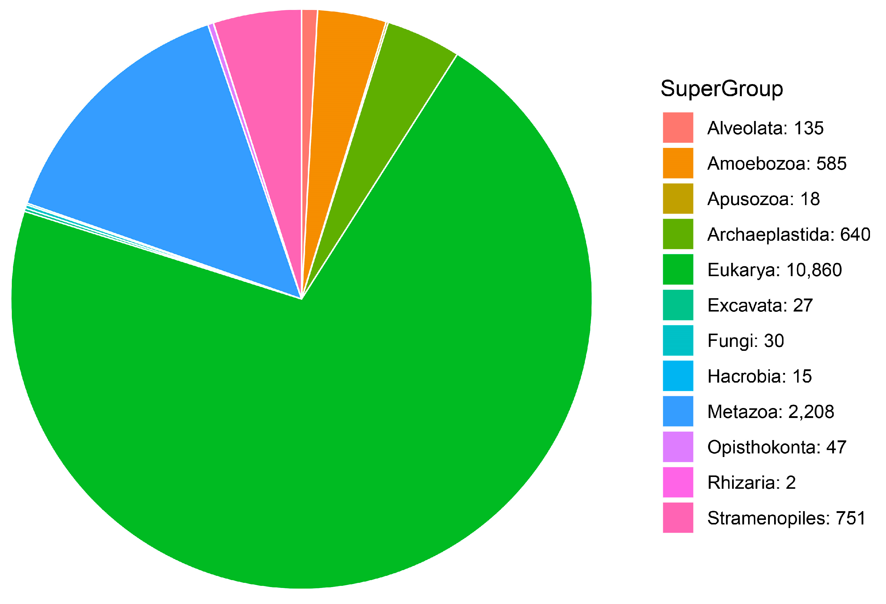
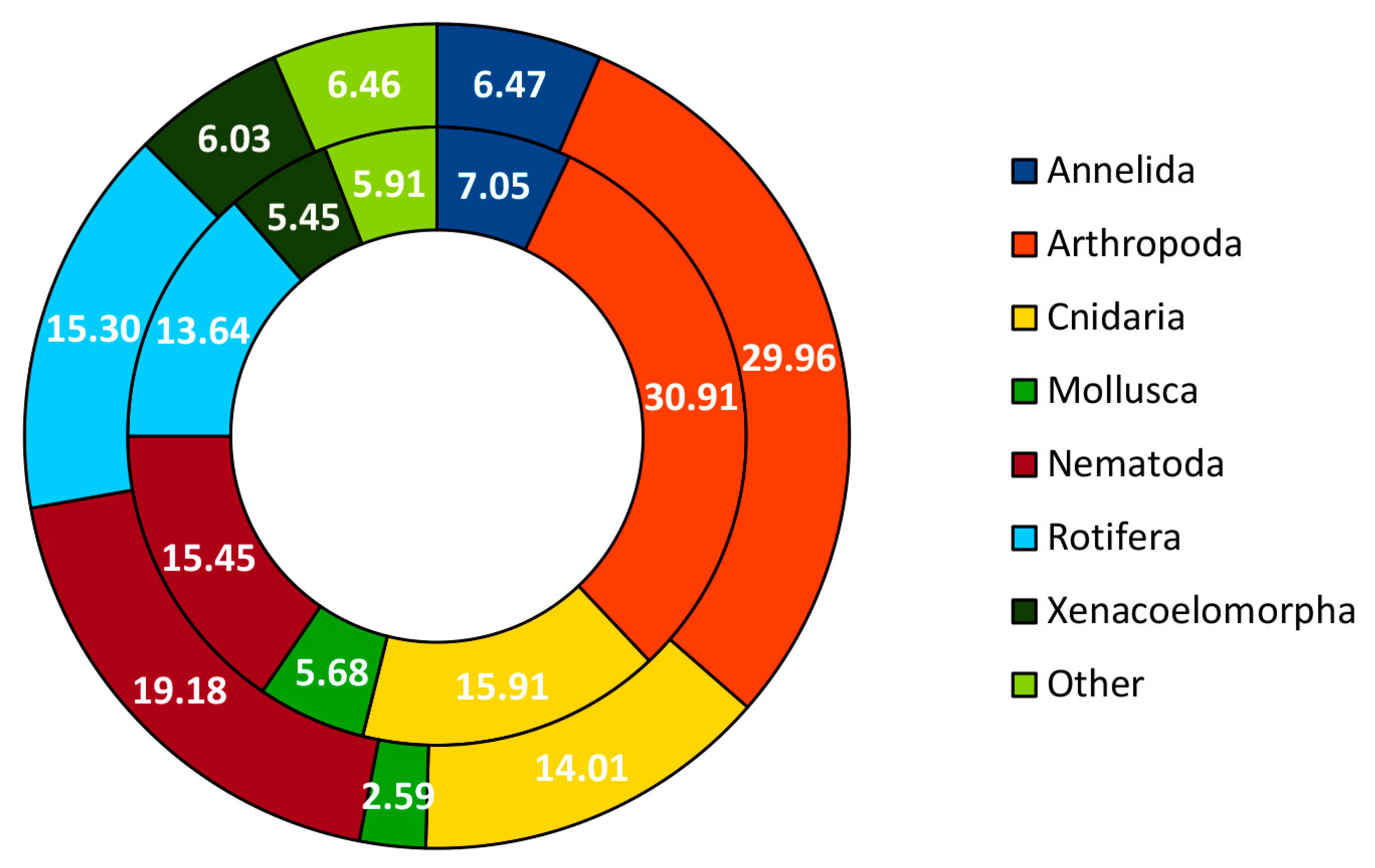
3.1. Community Profile

The MiSeq run produced 15,497,229 reads. After the cleaning and filtering processes, the final dataset obtained consisted of 15,318 MOTUs comprising 2,068,065 reads and 477,073 unique sequences. Most reads were lost during paired-end alignment, demultiplexing and quality filtering steps (>4,600,000 reads lost) and, particularly, during the length filter step (>7,100,000 reads lost), which is attributable to the amplification of non-eukaryotic taxa with variable length of this fragment. We also note that 13,491 MOTUs were filtered out because they had only one read. Blanks and negative controls (six in total) had, on average, 520 reads per sample and, cumulatively, 3178 reads, which is negligible compared to the global mean number of reads per sample (22,979). The obtained MOTUs are listed in Table S2 (Supplementary Materials) with taxonomic information, number of reads per sample, and representative sequence of each MOTU.
We performed rarefaction curves in order to check if the sequencing depth was appropriate to capture MOTU richness in our samples. Figure S1 (Supplementary Materials) shows that, in general, a plateau in the number of MOTUs per sample was reached at ca. 20,000 reads. Therefore, our mean sequence depth (22,979 reads per sample) adequately captures most of the MOTUs present in our samples. We then performed a species accumulation curve to visualize the accumulation rate of new MOTUs with increasing sampling effort and to take into account between-sample heterogeneity. As can be seen in Figure S2 (Supplementary Information), the curve does not reach an asymptote after processing 90 samples, yet it begins to plateau. Consequently, carrying out additional sampling would incorporate more MOTUs to the dataset.
The clusters were distributed in 11 super-groups: Alveolata, Rhizaria, Metazoa, Stramenopiles, Amoebozoa, Hacrobia, Fungi, Archaeplastida, Apusozoa, Opisthokonta (other than Metazoa and Fungi) and Excavata. However, there were 10,860 MOTUs (70.9% of the total) assigned to the broad category Eukarya (Table S2), which means that only the remaining 4458 MOTUs (comprising 880,696 reads) found a super-group or lower-level hit in the reference database. Of those 4458 MOTUs, Metazoa was the super-group with the highest number of MOTUs, and it accounted for 49.53% (2208) of the clusters. Stramenopiles and Archaeplastida were the second and third super-groups with the highest number of MOTUs (751 and 640, respectively). Figure 2 shows the total number of MOTUs per super-group, including those MOTUs assigned to the broad category Eukarya.
We identified 13 phyla among the metazoans: Annelida, Arthropoda, Bryozoa, Chordata, Cnidaria, Echinodermata, Mollusca, Nematoda, Nemertea, Platyhelminthes, Porifera, Rotifera and Xenacoelomorpha. A phylum level assignment could not be done for a substantial proportion of MOTUs (71.83%). Arthropoda, Nematoda and Cnidaria were the metazoan phyla with the highest number of MOTUs (196, 109 and 88, respectively). Figure 3 shows the total number of MOTUs per metazoan phylum, including unassigned MOTUs (i.e., those that could not be assigned at the phylum or lower level).
Frequencies of the taxonomic ranks at which MOTUs in our dataset were assigned by the ecotag procedure (excluding MOTUs assigned to Eukarya) are shown in Table 2. The three most frequent categories were, in this order, super-group, species and class, which collectively represent 79% of assignments. Only one fifth of the MOTUs were assigned at the lower taxonomic categories, that is, species and genus. Additionally, Table 2 shows the distribution of the 841 super-group MOTUs assigned to species, where Amoebozoa accounts for the majority of MOTUs assigned to this rank.
Taxonomic assignment frequencies of metazoan MOTUs (excluding unassigned) are given in Table 3. The main taxonomic categories that could be assigned were order and species; the latter represented 21.06% of the reads assigned to metazoans (excluding unassigned). Regarding the distribution of the 131 MOTUs assigned to species, it is worth noting that three phyla, Echinodermata, Nemertea and Platyhelminthes, did not have any MOTU assigned to this category and that the majority of the assignments corresponded to Rotifera.
Regarding the percentage of similarity between the clusters generated by the metabarcoding pipeline and the best hit in the customized reference database, Fungi had the highest mean percentage among super-groups, whereas Excavata had the lowest (86.49% and 73.82%, respectively). It is interesting to highlight that in Metazoa, the super-group with the highest number of MOTUs, assignments were made at a mean percentage of similarity of 78.52%. There are two metazoan phyla with assignments made at mean percentages above 95% similarity: Chordata and Echinodermata. However, the number of MOTUs included in each taxonomic group are four and one, respectively. The percentage of similarity in the most abundant phylum, Arthropoda, also fell below the 80% similarity threshold (79.85%), whereas the second and third, Nematoda and Cnidaria, were above it (81.67% and 84.41%).

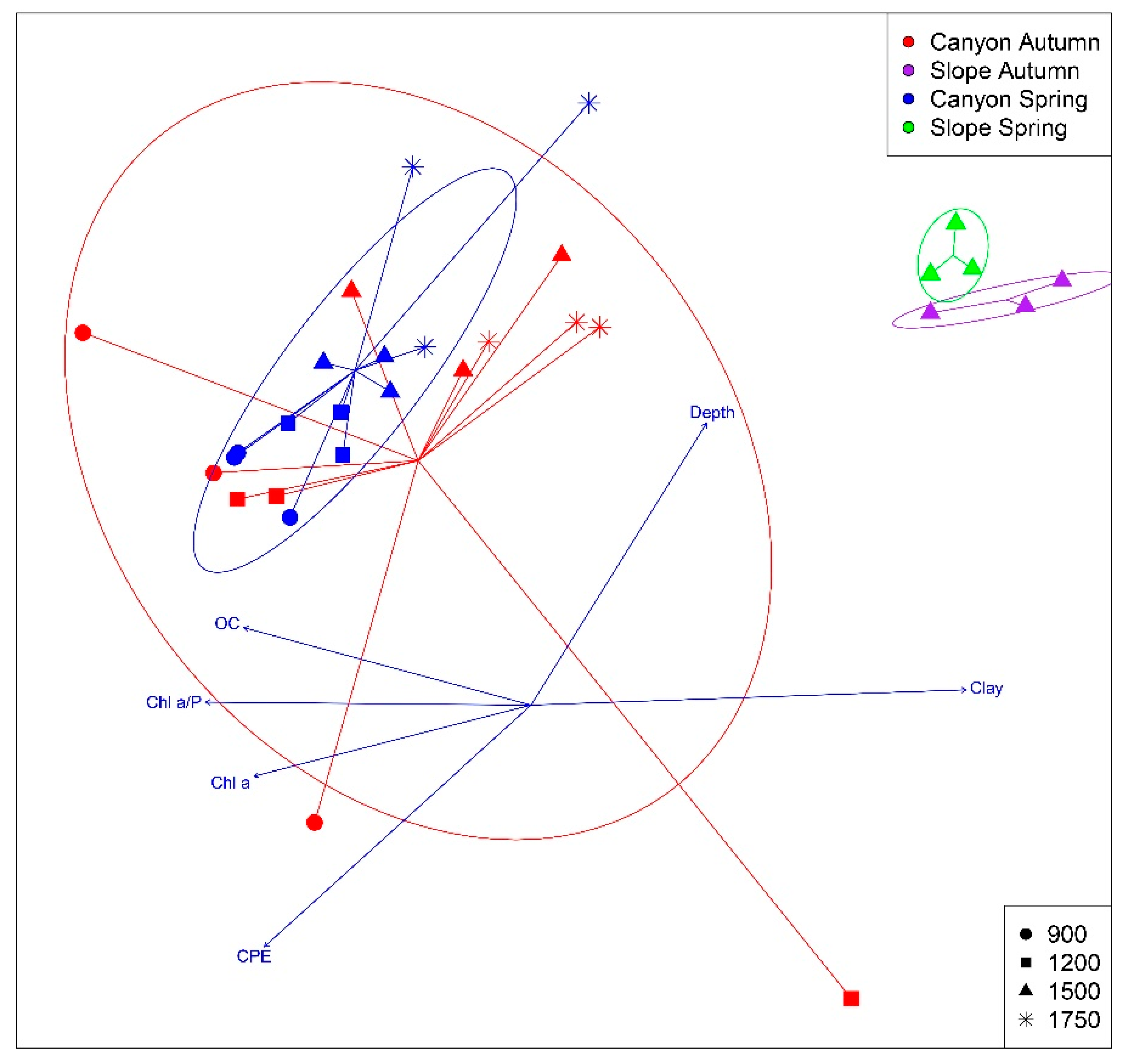
3.2. Spatio-temporal Patterns

We processed 90 samples, 45 from the autumn period and 45 from the spring one, obtained in two consecutive cruises. Regarding the vertical distribution of taxa of the global dataset by sediment layer, and considering all MOTUs (15,318), diversity decreased following the sediment profile. The highest diversity was found in the most superficial layer (layer A, the first cm of sediment), followed by the intermediate layer (layer B, second cm of the sediment) and, finally, by the deepest one (layer C, third to fifth cm of the sediment), with 12,399, 9025 and 6495 MOTUs, respectively. Therefore, as shown in Figure 4, ca. 80% of all MOTUs were present in layer A; ca. 60% in layer B; and ca. 40% in layer C. It is interesting to note that the number of exclusive taxa per layer also decreased markedly as we moved deeper into the sediment profile, from 29.1%, to 9.4%, and to 5.6% in the three layers. The 26.3% of MOTUs were shared by the three sediment layers. In metazoans, the total number of MOTUs also decreased from layer A to C (1768, 1271 and 926 MOTUs, respectively).
Considering MOTU richness per layer and sample, the values also diminish with sediment layer depth (476 ± 21, 348 ± 22, and 261 ± 20, for the first, second, and third to fifth centimetre, respectively). These differences in MOTU richness per sample were significant (one-way analysis of variance with corer as a repeated-measures factor, p < 0.001, Table S3 of Supplementary Materials). All between-layer pairwise comparisons were also highly significant (p < 0.001)
A non-metric multidimensional scaling (or nMDS) analysis based on the presence/absence data (Jaccard index) of the three sediment layers (with the three replicates of each locality pooled and rarefied to the lowest number of reads) is shown in Figure 5. The samples tended to group by layer, even though there was an overlap between the inertia ellipses of consecutive layers. It is interesting to note that, in each layer, the samples from the open slope (represented by triangles) appeared to be separated from the samples from the canyon and to be closer to the samples from the open slope of the other layers.
A PERMANOVA analysis of the factors layer (A, B, or C) and zone (canyon or open slope) showed a non-significant effect of the interaction, while both main factors were highly significant in structuring the community (Supplementary Materials, Table S4). PERMDISP tests showed significant heterogeneity in dispersion across levels of zone (p = 0.008), while the effect of layer was not due to differences in dispersion levels (p = 0.214). Pairwise comparisons between the three layers showed that the only significant difference in community structure was found between layers A and C (Table S4).
Overall, the number of MOTUs was slightly higher in autumn than in spring (6922 and 6738, respectively). Furthermore, after comparing the proportions of each group per season (Figure 6) no major differences were observable in the resulting seasonal communities, depicting a stable community over time. The breakdown of proportions of super-groups at each depth level and season is shown in Figure S3 of Supplementary Materials.
Regarding Metazoa, autumn was the season with the highest number of MOTUs compared to spring (1714 vs. 1596). The proportion of the different phyla in the community remains fairly constant over time (Figure 7). However, in Nematoda the number of MOTUs notably increased in spring (from 68 to 89). Likewise, in Rotifera the MOTU richness increased from 60 in autumn to 71 in spring. By contrast, in the phylum Mollusca, the number of MOTUs decreased by half in spring (from 25 to 12). Platyhelminthes were only represented in spring, and Echinodermata in autumn, albeit with only one MOTU each. The breakdown of proportions of metazoan phyla at each depth level and season is shown in Figure S3 of Supplementary Materials.
The patterns of MOTU richness per sample (Table S1) showed that, even if the total number of MOTUs found was slightly higher in autumn, the number of MOTUs per sample (with the three layers pooled and rarefied to a common number of reads) was, in general, higher in spring (2138 ± 144, mean ± SE) than in autumn (1750 ± 165). These differences in MOTU richness were not, however, significant (two-way ANOVA with station and season, no significant effects, Table S3).
With respect to the spatial distribution inside the canyon, the number of MOTUs decreased with depth, from the shallow stations located at 900 m depth to the deepest ones at 1750 m depth (7892, 7441, 7081 and 6173 MOTUs, respectively), and the same pattern was found for the metazoans (1149, 1068, 965 and 872 MOTUs, respectively). However, it is interesting to point out that the lowest number of MOTUs corresponded to the stations located in the open slope, at 1500 m depth (4840 total MOTUs, and 650 metazoan MOTUs).
When comparing MOTU richness per sample (the three layers pooled, Table S1) between the open slope and the equivalent depth in the canyon (1500 m), the former had lower values (1537 ± 115 vs. 2091 ± 162), and this difference was significant (one-way ANOVA, p = 0.017, Table S3). Finally, and similarly to what happened with the total number of MOTUs, MOTU richness per sample within the canyon showed a decreasing trend with depth (2146 ± 323, 2171 ± 358, 2092 ± 162, and 1774 ± 202 MOTUs at 900, 1200, 1500, and 1750 m, respectively). The differences, however, were not significant (ANOVA, p = 0.728, Table S3).
A nMDS was carried out in order to analyze spatio-temporal patterns between both localities and seasons (the three layers of each sample pooled), and is displayed in Figure 8. The most evident pattern of this ordination was the clear separation between samples from the Blanes canyon and the ones belonging to the open slope, with clearly separated inertia ellipses, which means that the community composition captured was different. When analysing the data per season, we can see that, even though the centroids of the inertia ellipses per season were separated, there was an overlap in their areas.
PERMANOVA tests performed using season and zone (canyon, open slope) as factors showed a non-significant interaction term and a significant effect of both main factors (Supplementary Materials Table S5). The PERMDISP test showed a significant outcome for zone, but not for season. This indicates that the zone effect is attributable to differences in sample dispersion among the levels of this factor (Table S5).
We then proceeded with only samples from the canyon and performed a new PERMANOVA test, with season and depth as factors. Again, there was no significant interaction term but both main factors had a significant effect in structuring the analysed community (Supplementary Materials Table S6). These effects were not due to the dispersion of the samples, as the corresponding PERMDISP tests reflected. The results of the pairwise tests between depths revealed statistically significant differences between all depth comparisons except for 900 vs. 1200 m and 1500 vs. 1750 m (Table S6).
The forward stepwise regression analysis included six environmental variables (Table S1) in the model that was retained. The variables Sand, Silt and Total Nitrogen (TN) and carbon/nitrogen ratio (C/N) were left out as redundant. The final model explained a significant proportion of the variation in distances (Jaccard index) between samples (r2 = 0.428, p < 0.001). The selected variables were plotted as vectors in the nMDS (Figure 8). When considered individually, all variables had a significant correlation with the ordination of the data (Table 4).

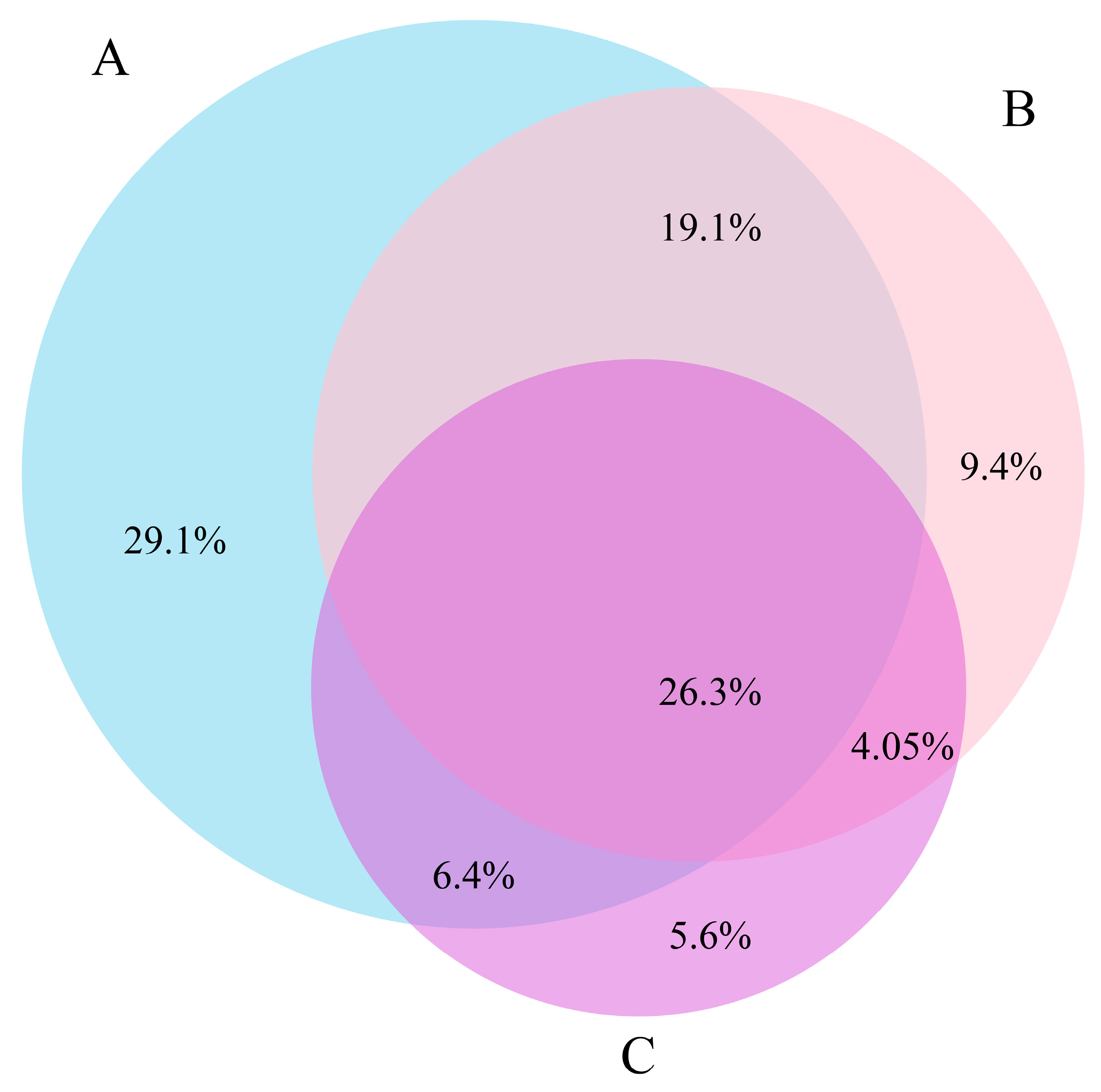
3.3. COI-18S Comparison

The final dataset of Guardiola et al. [31] consisted of 4953 MOTUs and 4,685,457 reads. It was compared to our dataset of 4458 MOTUs and 880,696 reads that excluded those that could not be assigned to super-group or lower level, and both datasets were rarefied to the lowest number of reads (for comparability reasons, see Methods). Figure S4 (Supplementary Materials) shows the proportion of eukaryotic MOTUs assigned to each rank with the COI (present work) and 18S [31] markers. When using 18S, species is the most frequent rank, with the rest of MOTUs distributed evenly among the other categories (except for a poor representation of phylum-level assignments). However, with COI, there is an outstanding presence of MOTUs assigned only to super-group, which is almost three times higher than with 18S. The second most frequent rank is species.
Metazoa appeared as the most diverse super-group in both datasets, but the second and third positions differed: Alveolata and Rhizaria in the 18S dataset, and Stramenopiles and Archaeplastida in the COI dataset. It is interesting to note that Alveolata and Rhizaria occupied the fifth and eleventh position (the latter with only two MOTUs) in the COI dataset, and Stramenopiles and Archaeplastida were the fourth and eighth most diverse taxa in the 18S dataset.
With respect to metazoans, despite the fact that more MOTUs were detected with COI (2208) than with 18S (1659), the dataset from Guardiola et al. [31] contained sequences from 20 metazoan phyla, as compared to only 13 phyla in our dataset. Another important difference was that, with 18S, only 14.83% of metazoan MOTUs could not be assigned at least to phylum level, while with COI 71.83% of MOTUs remained unassigned. The five most diverse phyla in the 18S dataset were, in order, Nematoda, Arthropoda, Annelida, Platyhelminthes and Cnidaria, whereas in the COI dataset they were, respectively, Arthropoda, Nematoda, Cnidaria, Annelida and Xenacoelomorpha. It is interesting to highlight that targeting the 18S rRNA gene enabled the assignment of 651 MOTUs to Nematoda, whereas only 109 could be assigned to the same taxon when targeting the COI gene. Moreover, it is striking that Platyhelminthes, the fourth most abundant phylum in the 18S dataset (109 MOTUs), was represented by only one MOTU in the COI dataset.
Diversity in the three layers of the sediment analysed with the 18S gene also decreased following the depth gradient, as well as the number of exclusive MOTUs per layer.
When comparing the nMDS based on presence/absence data for the three layers of sediment obtained with COI and 18S (Figure S5 in Supplementary Materials), we observed that, disregarding the type of marker, samples were grouped following the gradient in layer depth, and samples from the open slope were also set apart. The two configurations were similar, as shown by the significant correlation of the underlying Jaccard distance matrices (Mantel test, r = 0.681 p < 0.001). The ordinations provided by both markers in the nMDS by season and zone (Figure S6 in Supplementary Materials) showed a similar configuration of the samples (Mantel test of the distance matrices, r = 0.793, p < 0.001). They had in common the clear distinction between samples from the open slope and from the canyon (even though this was clearer in the COI ordination). Focusing on the canyon, there was a coincidence in both ordinations: the centroids of the inertia ellipses representing samples from different seasons appeared to be separated, but the inertia ellipses overlapped, and there appeared to be a higher heterogeneity in samples from autumn in both cases.

4. Discussion

The amplification of the COI marker yielded a high number of MOTUs (15,318) in the deep-sea sediment communities analysed, yet the number of MOTUs that received assignments below the Eukarya category was comparatively small (4458). Therefore, 70.9% of the eukaryotic clusters remained unassignable. There was also a generally low similarity between sequences in our dataset and their best hit in the reference database (ca. 80% on average, 82% for metazoans). In fact, less than 1% of MOTUs were assigned at similarities above 90%. The number of unassigned MOTUs, and the overall similarity of MOTUs to their respective best-matches in the reference database, points out a blatant lack of completeness of this reference database. Furthermore, assignments below the Eukarya category were made, in general, at high taxonomic levels, with 53.3% of assignments corresponding to the super-group and phylum levels. At the species level, 52.32% of assignments belonged to organisms of only one super-group, Amoebozoa, which had been the object of remarkable barcoding efforts (e.g., [57,58,59]). All this evidence confirms previous reports that there are major gaps in reference databases that use COI as a marker regarding sediment communities from both marine and freshwater environments [23,60], or even regarding marine organisms in general [33,61]. Notwithstanding, one of the advantages of metabarcoding is that taxonomic identification can only improve as reference databases are updated. Thus, re-analysis of our dataset could yield a more precise taxonomic profiling in the future, when more complete databases become available.
We found a high taxonomic diversity in our samples, with representatives of 11 super-groups, although only four of them, Metazoa, Stramenopiles Archaeplastida and Amoebozoa, accounted for 93.85% of the total number of MOTUs. With respect to the metazoans, 13 phyla were represented in our dataset, with the four main groups (Arthropoda, Nematoda, Cnidaria and Rotifera) accounting for 76.05% of the MOTUs. The majority of MOTUs present in the samples was retrieved during the processing, providing reliable MOTU richness values, as shown by rarefaction curves reaching, in general, a plateau. Nevertheless, the rate of accumulation of new MOTUs (or organisms) as more samples were analysed was far from acquiring an asymptotic shape. Consequently, sampling efforts should improve by increasing the number of replicates per locality in order to carry out exhaustive community inventories on such hyperdiverse communities [62].
MOTU richness per sample decreased significantly following the vertical structure of the sediment, from the 1st cm down to the fraction that comprised the 3rd to 5th cm. The densities of meiofauna are known to decrease over the first centimetres of sediment [63,64,65], and changes in relative proportions of different groups occur as well [64]. Overall, layer A hosted almost twice the MOTUs found in layer C and 27.21% more MOTUs than layer B, and only 26.3% of all MOTUs were detected in the three layers. Each layer seemed to harbour distinct communities in a nMDS ordination, although only layers A and C differed significantly in a PERMANOVA analysis of community structure. PERMANOVA analyses also showed that layer and zone (canyon or open slope) were the significant factors structuring the studied community, a result in agreement with what is found for nematode communities in this same area [65]. We cannot reliably link sediment depth with age of the communities, as DNA residence times in deep-sea sediments are of the order of 10 years in the top centimetre [26], and the relatively long marker used (313 bp) may degrade even faster. Additionally, cascading events [11] can periodically alter the vertical structure of the sediments, so we expect the sampled communities to be recent.
There were no significant changes in overall MOTU richness across seasons. PERMANOVA analyses, on the other hand, detected significant differences in community structure between seasons, thus revealing a temporal component of variation. However, a complete seasonal cycle with more replicates would be needed to reliably assess seasonal patterns in these communities. The role of seasonal variation in faunal assemblages in the same canyon has been highlighted for megafauna biomass [66] and biological cycles [67], and it is attributable to changes in downward transport of organic matter [67,68], which are in turn likely influenced by seasonal cascading events [11].
The nMDS ordination and PERMANOVA results showed that the community found in the canyon was significantly different from that in the adjacent open slope. Comparisons of MOTU richness per sample at equivalent depths (1500 m) revealed a significantly higher richness (ca. 36% higher) in the canyon relative to the open slope. The Blanes canyon is subject to higher hydrodynamics and sedimentary processes than the open slope, which is a more stable habitat [63]. For megafauna, a lower species richness and diversity in the open slope than in the canyon, as well as a different community structure, have been reported [66,69]. Likewise, the canyon hosted, in general, more abundant and diverse nematode assemblages than the open slope [65].
Along the canyon, there was a trend towards diminishing MOTU richness per sample with depth, which is consistent with previous findings (reviewed in Danovaro et al. [7], Costello and Chaudhary [70]). However, the idea of a peak in diversity at intermediate depths has also been put forward [62], and the maxima of megafaunal biomass and meiofaunal densities have indeed been reported in the Blanes Canyon at intermediate depths [56,66]. Notwithstanding, the meiofaunal diversities have been reported to have a diminishing trend with depth in the canyon, but this pattern was blurred in spring, where storm-induced turbidity and increase in particle transport made communities more fluctuating [63]. As regards community structure, PERMANOVA revealed that depth was a significant structuring factor, and that the communities found at a given depth were significantly different from communities separated by one or two depth levels. A different community structure with depth in the main metazoan group, nematodes, was also noted by Roman et al. [65].
Out of a list of 10 environmental variables, six were selected as non-redundant and all of them correlated significantly with the ordination of the samples. The vectors of depth and percent clay (indicating granulometry) pointed to a similar direction in the ordination, opposite the other variables which are linked to the food signal in the sediment: pigments, (Chl a, Chl a/Phaeopigments, chloroplastic pigment equivalents) and organic carbon contents. Thus, a general pattern of decrease in particle size and in sedimentary food sources along the depth gradient seemed determinant in structuring sediment communities in this area. Highly significant relationships between meiofaunal parameters and variables related to food quantity and quality have been reported elsewhere in the Mediterranean [71], and the reliance of deep-sea species diversity on sediment particle characteristics and organic matter inputs is well established [62,72,73].
Our results were compared with those obtained from the same samples, but targeting the 18S rRNA gene [31] (note that the pipelines for both markers differed in some aspects, as detailed in Methods). We retrieved a larger number of MOTUs in the COI dataset (15,318) than found with the ribosomal marker (10,073 before the elimination of those that could not be assigned to super-group level), even though the final number of reads (after applying the bioinformatic pipeline) was much lower with COI (2,068,065) than with 18S (over 9,500,000). It can be noted that both studies used a full run of MiSeq with a similar initial output. Thus, COI detected 50% more MOTUs with only ca. one fifth of reads. This is coherent with previous findings [33,35,36,74], and is likely due to the much lower variability of the 18S gene, that underestimates the true number of species [35,75]. It can be noted here that the v7 region of the 18S rRNA gene targeted in Guardiola et al. [31] is comparatively less used in broad-range studies, compared to regions v1-2 and v9 [75]. However, the v7 region is also a hotspot of nucleotide variability within the 18S gene [76].
A second major difference was found in the taxonomic assignment performance. While leaving out MOTUs that could not be assigned to a super-group or lower rank reduced the list of 18S MOTUs to ca. one half, with COI it was reduced to less than one third. In addition, the taxonomic levels at which the assignment was made was consistently higher with COI (e.g., 71.8% of metazoans could not be assigned to phylum level, as compared to 14.8% with 18S). Again, this is related to the different variability of the markers. Thus, with 18S it is possible to identify a sequence to a lower taxonomic rank whenever a related sequence, even if it comes from a distant relative, is present in the reference database. Conversely, because sequence changes tend to saturate, identification with the hypervariable marker COI needs a closely related sequence to be present in the reference database. This is not the case for many organisms living in deep-sea ecosystems, particularly the small meio- and micro-organisms present in the sediments, with many groups poorly represented or absent altogether from the databases. The high variability of COI exacerbates the effects of these database gaps as close sequences are required, while, with 18S, gaps are more easily bridged.
A different matter is the degree of reliability of the low-level taxonomic assignments. The 18S marker is known to have a low taxonomic resolution for many eukaryotic groups [75]. In short, with 18S we trade the capacity for assigning more MOTUs thanks to its low variability with the low taxonomic reliability achieved (we cannot rely on low-level taxonomic assignments as several taxa can share the same sequence). With COI, we detect a much higher number of MOTUs (often more than nominal species [35]) at the cost of many of them remaining anonymous, but when a low-level assignment is made at high percent similarity, we can be reasonably sure that the correct species has been assigned.
Moreover, it is important to note that recovering DNA directly from sediments without any sieving allows the inclusion of many micro-eukaryotes poorly represented in the databases, thus diminishing assignment success. Not sieving also means that more organismal traces and extracellular DNA are retained, which has the risk of incorporating non-benthic organisms whose DNA has sunk to the bottom [28,77] or even non-marine DNA. It has been said that the deep-sea sediments constitute an archive of present and past marine biodiversity [78,79]. In this sense, selecting large DNA fragments, such as > 300 bp in the COI fragment amplified here, will favour the amplification of DNA from living (or recently dead) organisms as compared to the shorter (ca. 130 bp) fragment of the 18S used by Guardiola et al. [31], because longer DNA molecules tend to fragment and degrade faster over time [80].
Metazoa was, in both datasets, the most diverse super-group, but the second and third most MOTU-rich super-groups differed. Likewise, the five most diverse metazoan phyla were practically the same in both datasets, but in a different order and in different proportions. In addition, the 18S dataset included seven metazoan phyla not present in the COI dataset. Therefore, both markers can result in different taxonomic profiles. In addition to database completeness, primer bias or the differential capacity of the primers to bind to sequences of some groups can also be a concern when choosing a marker, as it has been pointed out that COI lacks true universal primers due to an excess of variability [81]. However, this problem has been ameliorated with the development of new sets of degenerate primers [82,83] such as the one used here targeting the second half of the standard barcode fragment [33,38]. For 18S, several primer pairs exist that target variable regions of the gene and are reasonably universal [76]. It is remarkable that, in spite of differences in numbers of MOTUs and taxonomic assignment success, the spatio-temporal patterns rendered by each marker were basically the same. Distance matrices obtained by both markers were highly correlated (Mantel tests), and sample ordinations (nMDS) were similar (Figures S5 and S6). The main trends were detected with both markers, both at the sediment layer level and in the spatio-temporal structures detected [31].
In summary, COI metabarcoding revealed a rich community in a deep-sea canyon of the Mediterranean Sea. Over 15,000 MOTUs were detected which, compared to ca. 17,000 marine species known in this sea [6], or 2805 estimated species in its deep-sea bottoms [7], testifies to both the diversity of the communities studied and our profound knowledge gap about the extent of marine diversity. A clear pattern of decreasing diversity with sediment layer depth was found. Seasonality was also detected, possibly linked to pulses of organic matter. Overall, the interplay of depth-related trends, such as a finer granulometry and decreasing food availability, seemed to drive the structure of the communities studied. Our results also suggest that, despite important differences in the performance of both markers, and the differential ability to recover some groups, COI can retrieve broadly the same ecological information than the more frequently used marker 18S from eDNA samples. The number of MOTUs retrieved is higher with COI, but the taxonomic assignment is poor compared to that obtained from 18S. The higher variability of COI makes it a more promising marker for developing high-resolution bioindicators of particular ecological conditions compared to 18S. These developments should rely, for the time being, on taxonomy-free methods, which would detect ecological shifts, even if the indicator sequences do not yet have a taxonomic identification. Finally, the applications of COI are being hampered by significant gaps in the reference databases for deep-sea organisms, which need to be filled in future barcoding projects, if taxonomy-based applications are to be developed.

Supplementary Materials

The following are available online at https://www.mdpi.com/1424-2818/12/4/123/s1, Figure S1: Rarefaction curves of the number of MOTUs obtained at increasing number of reads per sample. The red vertical line marks the overall mean number of reads per sample, Figure S2: MOTU accumulation curve as samples are added to the analysis. The shaded area represents the 95% confidence interval, Figure S3: Proportion of MOTUs of the different super-groups (a and b) and metazoan phyla (c and d), per sampling station (BC900, BC1290, BC1500, BC1750 and OS1500) and season (autumn and spring), Figure S4: Proportion of MOTUs assigned to the following taxonomic categories: super-group, phylum, class, order, family, genus and species, both in the COI restricted dataset and in the 18S dataset. Numbers correspond to the percentage of MOTUs that each group represents in each dataset, Figure S5: nMDS representations of the samples by layers (the three replicates per locality merged) conducted on the restricted COI dataset of 4458 MOTUs and the dataset of 4953 18SrDNA MOTUs from Guardiola et al. [31]. The stress values of the ordinations are 12.05% for COI and 13.09 for 18S, Figure S6: nMDS representation of the samples of the spatio-temporal study (the three layers of sediment merged) conducted on the restricted COI dataset of 4458 MOTUs and the dataset of 4953 18SrDNA MOTUs from Guardiola et al. [31]. The stress values of the ordinations are11.48% for COI and 9.97% for 18S, Table S1: Number of MOTUs found per sample (pooling the three layers) at each station and season (after rarefaction to the lowest number of reads), together with values of environmental variables. Percents of Clay, Silt and Sand, Chlorophyll a (Chl a), chloroplastic pigment equivalents (CPE), chlorophyll a divided by its degradation products (phaeopigments) (Chl a/P), organic carbon content (OC), total nitrogen content (TN), molar carbon-nitrogen ratio (C/N). Data from Roman et al. (2016), obtained during the same cruises and at the exact same sampling stations and dates as our data, Table S2: List of the original MOTUs with taxonomic information, number of reads per sample, number of unique sequences in the MOTU (depth), and the representative sequence of each MOTU, Table S3. A. Univariate repeated measures ANOVA of the effect of layer (A, B, C) on MOTU richness per sample. Individual corers are the repeated factor. Mauchly’s sphericity test passed (p = 0.945), so no correction was performed. B. Two-way ANOVA of the effects of season (autumn, spring) and station (BC900, BC1200, BC1500, BC1750, OS1500) on the number of MOTUs per sample. C. One-way ANOVA of the effects of zone (canyon, open slope) at a fixed depth of 1500 m on MOTU richness per sample. D. One-way ANOVA of the effects of depth (900, 1200, 1500 and 1750 m) on MOTU richness per sample in canyon stations (*: significant outcome), Table S4: PERMANOVA and PERMDISP tests of the factors layer (A, B, C) and zone (canyon, open slope) for the Jaccard index (*: significant values). The results for the permutational pairwise tests of levels of the factor layer are also provided (*: significant outcome after FDR correction), Table S5: PERMANOVA and PERMDISP tests of the effect of zone (canyon, open slope) and season (autumn, spring) for the Jaccard index. The three layers of each sample were pooled (*: significant values), Table S6: PERMANOVA and PERMDISP tests of the effects of season (autumn, spring) and depth on the samples from the Blanes Canyon for the Jaccard index (*: significant values). The results for the permutational pairwise tests of levels of the factor depth are also provided (*: significant outcome after FDR correction). The three layers of each sample were pooled.

Author Contributions

X.T.; K.P. and O.S.W. designed the study; M.G. conducted field work; M.G. and O.S.W. performed laboratory work; X.T. and K.P. contributed reagents and funding; S.A. and A.A. adapted and ran the bioinformatics pipeline; S.A. and X.T. performed statistical analyses; S.A. wrote the first draft of the manuscript; all authors contributed to the manuscript and agreed to the submitted version. All authors have read and agreed to the published version of the manuscript.

Funding

The sampling has been done in the framework of the DOSMARES project (CTM2010-21810) of the Spanish Government. This research has been funded by project PopCOmics CTM2017-88080 (MCIU/AEI/FEDER, UE) of the Spanish Government. This is a contribution from the Consolidated Research Group “Benthic Biology and Ecology” SGR2017-1120 of the Catalan Government.

Acknowledgments

We are indebted to Sara Roman, Chiara Romano and Marta Segura for their help in sample collection during the DOSMARES cruises. Sara Roman helped also with literature on deep-sea processes.

Conflicts of Interest

The authors declare no conflict of interest.

References

  1. Eakins, B.W.; Sharman, G.F. Volumes of the World’s Oceans from ETOPO1. NOAA National Geophysical Data Center, Boulder, CO. 2010. Available online: https://www.ngdc.noaa.gov/mgg/global/etopo1_ocean_volumes.html (accessed on 16 November 2019).
  2. Costello, M.J.; Cheung, A.; De Hauwere, N. Topography statistics for the surface and seabed area, volume, depth and slope, of the world’s seas, oceans and countries. Environ. Sci. Technol. 2010, 44, 8821–8828. [Google Scholar] [CrossRef] [PubMed]
  3. Ramirez-Llodra, E.; Tyler, P.A.; Baker, M.C.; Bergstad, O.A.; Clark, M.R.; Escobar, E.; Levin, L.A.; Lenaick, M.; Ashley, A.R.; Craig, R.S.; et al. Man and the last great wilderness: Human impact on the deep sea. PLoS ONE 2011, 6, e22588. [Google Scholar] [CrossRef] [PubMed] [Green Version]
  4. Danovaro, R.; Snelgrove, P.V.R.; Tyler, P. Challenging the paradigms of deep-sea ecology. Trends Ecol. Evol. 2014, 29, 465–475. [Google Scholar] [CrossRef] [PubMed]
  5. Danovaro, R.; Fanelli, E.; Canals, M.; Ciuffardi, T.; Fabri, M.-C.; Taviani, M.; Argyrou, M.; Azzurro, E.; Bianchelli, S.; Cantafaro, A.; et al. Towards a marine strategy for the deep Mediterranean Sea: Analysis of current ecological status. Mar. Policy 2020, 112. [Google Scholar] [CrossRef]
  6. Coll, M.; Piroddi, C.; Steenbeek, J.; Kaschner, K.; Ben Rais Lasram, F.; Aguzzi, J.; Ballesteros, E.; Bianchi, C.N.; Corbera, J.; Dailianis, T.; et al. The Biodiversity of the Mediterranean Sea: Estimates, Patterns, and Threats. PLoS ONE 2010, 5, e11842. [Google Scholar] [CrossRef] [Green Version]
  7. Danovaro, R.; Company, J.B.; Corinaldesi, C.; D’Onghia, G.; Galil, B.; Gambi, C.; Gooday, A.J.; Lampadariou, N.; Luna, G.M.; Morigi, C.; et al. Deep-Sea Biodiversity in the Mediterranean Sea: The Known, the Unknown, and the Unknowable. PLoS ONE 2010, 5, e11832. [Google Scholar] [CrossRef] [Green Version]
  8. Harris, P.; Whiteway, T. Global distribution of large submarine canyons: Geomorphic differences between active and passive continental margins. Mar. Geol. 2011, 285, 69–86. [Google Scholar] [CrossRef]
  9. Guillén, J.; Bourrin, F.; Palanques, A.; Durrieu de Madron, X.; Puig, P.; Buscail, R. Sediment dynamics during wet and dry storm events on the Têt inner shelf (SW Gulf of Lions). Mar. Geol. 2006, 234, 129–142. [Google Scholar] [CrossRef]
  10. Bonnin, J.; Heussner, S.; Calafat, A.; Fabres, J.; Palanques, A.; Durrieu de Madron, X.; Canals, M.; Puig, P.; Avril, J.; Delsaut, N. Comparison of horizontal and downward particle fluxes across canyons of the Gulf of Lions (NW Mediterranean): Meteorological and hydrodynamical forcing. Cont. Shelf Res. 2008, 28, 1957–1970. [Google Scholar] [CrossRef]
  11. Canals, M.; Puig, P.; Durrieu de Madron, X.; Heussner, S.; Palanques, A.; Fabres, J. Flushing submarine canyons. Nature 2006, 444, 354–357. [Google Scholar] [CrossRef]
  12. Heussner, S.; Durrieu de Madron, X.; Calafat, A.; Canals, M.; Carbonne, J.; Delsaut, N.; Saragoni, G. Spatial and temporal variability of downward particle fluxes on a continental slope: Lessons from an 8-yr experiment in the Gulf of Lions (NW Mediterranean). Mar. Geol. 2006, 234, 63–92. [Google Scholar] [CrossRef]
  13. Ulses, C.; Estournel, C.; Puig, P.; Durrieu de Madron, X.; Marsaleix, P. Dense shelf water cascading in the northwestern Mediterranean during the cold winter 2005: Quantification of the export through the Gulf of Lion and the Catalan margin. Geophys. Res. Lett. 2008, 35. [Google Scholar] [CrossRef] [Green Version]
  14. Canals, M.; Company, J.B.; Martín, D.; Sànchez-Vidal, A.; Ramírez-Llodra, E. Integrated study of Mediterranean deep canyons: Novel results and future challenges. Prog. Oceanogr. 2013, 118. [Google Scholar] [CrossRef] [Green Version]
  15. Lopez-Fernandez, P.; Calafat, A.; Sanchez-Vidal, A.; Canals, M.; Mar Flexas, M.; Cateura, J.; Company, J.B. Multiple drivers of particle fluxes in the Blanes submarine canyon and southern open slope: Results of a year round experiment. Prog. Oceanogr. 2013, 118, 95–107. [Google Scholar] [CrossRef]
  16. Puig, P.; Martín, J.; Masqué, P.; Palanques, A. Increasing sediment accumulation rates in La Fonera (Palamós) submarine canyon axis and their relationship with bottom trawling activities. Geophys. Res. Lett. 2015, 42, 8106–8113. [Google Scholar] [CrossRef] [Green Version]
  17. Paradis, S.; Puig, P.; Sanchez-Vidal, A.; Masqué, P.; Garcia-Orellana, J.; Calafat, A.; Canals, M. Spatial distribution of sedimentation-rate increases in Blanes Canyon caused by technification of bottom trawling fleet. Prog. Oceanogr. 2018, 169, 241–252. [Google Scholar] [CrossRef]
  18. Zúñiga, D.; Flexas, M.M.; Sanchez-Vidal, A.; Coenjaerts, J.; Calafat, A.; Jordà, G.; Company, J.B. Particle fluxes dynamics in Blanes submarine canyon (Northwestern Mediterranean). Prog. Oceanogr. 2009, 82, 239–251. [Google Scholar] [CrossRef]
  19. Snelgrove, P.V.R. An ocean of discovery: Biodiversity beyond the census of marine life. Planta Med. 2016, 82, 790–799. [Google Scholar] [CrossRef] [Green Version]
  20. Bohmann, K.; Evans, A.; Gilbert, M.T.P.; Carvalho, G.R.; Creer, S.; Knapp, M.; Yu, D.W.; de Bruyn, M. Environmental DNA for wildlife biology and biodiversity monitoring. Trends Ecol. Evol. 2014, 29, 358–367. [Google Scholar] [CrossRef]
  21. Creer, S.; Deiner, K.; Frey, S.; Porazinska, D.; Taberlet, P.; Thomas, W.K.; Potter, C.; Bik, H.M. The ecologist’s field guide to sequence-based identification of biodiversity. Methods Ecol. Evol. 2016, 7, 1008–1018. [Google Scholar] [CrossRef]
  22. Lodge, D.M.; de Vere, N.; Pfrender, M.E.; Bematchez, L. Environmental DNA metabarcoding: Transforming how we survey animal and plant communities. Mol. Ecol. 2017, 26, 5872–5895. [Google Scholar] [CrossRef]
  23. Sinniger, F.; Pawlowski, J.; Harii, S.; Gooday, A.J.; Yamamoto, H.; Chevaldonné, P.; Cedhagen, T.; Carvalho, G.; Creer, S. Worldwide Analysis of Sedimentary DNA Reveals Major Gaps inTaxonomic Knowledge of Deep-SeaBenthos. Front. Mar. Sci. 2016, 3, 92. [Google Scholar] [CrossRef] [Green Version]
  24. Brandt, M.I.; Trouche, B.; Quintric, L.; Wincker, P.; Poulain, J.; Arnaud-Haond, S. A flexible pipeline combining bioinformatic correction tools for prokaryotic and eukaryotic metabarcoding. bioRxiv 2019. [Google Scholar] [CrossRef] [Green Version]
  25. Taberlet, P.; Coissac, E.; Pompanon, F.; Brochmann, C.; Willerslev, E. Towards next-generation biodiversity assessment using DNA metabarcoding. Mol. Ecol. 2012, 21, 2045–2050. [Google Scholar] [CrossRef] [PubMed]
  26. Dell’Anno, A.; Danovaro, R. Extracellular DNA plays a key role in deep-sea ecosystem functioning. Science 2005, 309, 2179. [Google Scholar] [CrossRef] [PubMed]
  27. Stoeck, T.; Behnke, A.; Christen, R.; Amaral-Settler, L.; Rodriguez-Mora, M.J.; Chistoserdov, A.; Orsi, W.; Edgcomb, V.P. Massively parallel tag sequencing reveals the complexity of anaerobic marine protistan communities. BMC Biol. 2009, 7, 72. [Google Scholar] [CrossRef] [Green Version]
  28. Pawlowski, J.; Christen, R.; Lecroq, B.; Bachar, D.; Shahbazkia, H.R.; Amaral-Zettler, L.; Guillou, L. Eukaryotic Richness in the Abyss: Insights from Pyrotag Sequencing. PLoS ONE 2011, 6, e18169. [Google Scholar] [CrossRef]
  29. Bik, H.M.; Porazinska, D.L.; Creer, S.; Caporaso, J.G.; Knight, R.; Thomas, W.K. Sequencing our way towards understanding global eukaryotic biodiversity. Trends Ecol. Evol. 2012, 27, 233–243. [Google Scholar] [CrossRef] [Green Version]
  30. Guardiola, M.; Uriz, M.J.; Taberlet, P.; Coissac, E.; Wangensteen, O.S.; Turon, X. Deep-Sea, Deep-Sequencing: Metabarcoding Extracellular DNA from Sediments of Marine Canyons. PLoS ONE 2015, 10, e0139633. [Google Scholar] [CrossRef] [Green Version]
  31. Guardiola, M.; Wangensteen, O.S.; Taberlet, P.; Coissac, E.; Uriz, M.J.; Turon, X. Spatio-temporal monitoring of deep-sea communities using metabarcoding of sediment DNA and RNA. PeerJ 2016, 4, e2807. [Google Scholar] [CrossRef] [Green Version]
  32. Brannock, P.M.; Learman, D.R.; Mahon, A.R.; Santos, S.R.; Halanych, K.M. Meiobenthic community composition and biodiversity along a 5500 km transect of Western Antarctica: A metabarcoding analysis. Mar. Ecol. Prog. Ser. 2018, 603, 47–60. [Google Scholar] [CrossRef]
  33. Wangensteen, O.S.; Palacín, C.; Guardiola, M.; Turon, X. DNA metabarcoding of littoral hard-bottom communities: High diversity and database gaps revealed by two molecular markers. PeerJ 2018, 6, e4705. [Google Scholar] [CrossRef] [PubMed]
  34. Hu, M.; Chilton, N.B.; Zhu, X.; Gasser, R.B. Single-strand conformation polymorphism-based analysis of mitochondrial cytochrome c oxidase subunit 1 reveals significant substructuring in hookworm populations. Electrophoresis 2002, 23, 27–34. [Google Scholar] [CrossRef]
  35. Tang, C.Q.; Leasi, F.; Obertegger, U.; Kieneke, A.; Barraclough, T.G.; Fontaneto, D. The widely used small subunit 18S rDNA molecule greatly underestimates true diversity in biodiversity surveys of the meiofauna. Proc. Natl. Acad. Sci. USA 2012, 109, 16208–16212. [Google Scholar] [CrossRef] [PubMed] [Green Version]
  36. Cowart, D.A.; Pinheiro, M.; Mouchel, O.; Maguer, M.; Grall, J.; Miné, J.; Arnaud-Haond, S. Metabarcoding is powerful yet still blind: A comparative analysis of morphological and molecular surveys of seagrass communities. PLoS ONE 2015, 10, e0117562. [Google Scholar] [CrossRef] [PubMed] [Green Version]
  37. Turon, X.; Antich, A.; Palacín, C.; Præbel, K.; Wangensteen, O.S. From metabarcoding to metaphylogeography: Separating the wheat from the chaff. Ecol. Appl. 2019, 30, e02036. [Google Scholar] [CrossRef] [PubMed]
  38. Leray, M.; Yang, J.Y.; Meyer, C.P.; Mills, S.C.; Agudelo, N.; Ranwez, V.; Boehm, J.; Machida, R.J. A new versatil primer set targeting a short fragment of the mithocondrial COI region for metabarcoding metazoan diversity: Application for characterizing coral reef fish gut contents. Front. Zool. 2013, 10, 34. [Google Scholar] [CrossRef] [PubMed] [Green Version]
  39. Ratnasingham, S.; Hebert, P.D.N. Bold: The Barcode of Life Data System (www.barcodinglife.org). Mol. Ecol. Notes 2007, 7, 355–364. [Google Scholar] [CrossRef] [Green Version]
  40. Lastras, G.; Canals, M.; Amblas, D.; Lavoie, C.; Church, I.; De Mol, B.; Duran, R.; Calafat, A.M.; Hughes-Clarke, J.E.; Smith, C.J.; et al. Understanding sediment dynamics of two large submarine valleys from seafloor data: Blanes and La Fonera canyons, northwestern Mediterranean Sea. Mar. Geol. 2011, 280, 20–39. [Google Scholar] [CrossRef]
  41. Amblas, D.; Canals, M.; Urgeles, R.; Lastras, G.; Liquete, C.; Hughes-Clarke, J.E.; Calafat, A.M. Morphogenetic mesoscale analysis of the northeastern Iberian margin, NW Mediterranean Basin. Mar. Geol. 2006, 234, 3–20. [Google Scholar] [CrossRef]
  42. Geller, J.; Meyer, C.; Parker, M.; Hawk, H. Redesign of PCR primers for mitochondrial cytochrome c oxidase subunit I for marine invertebrates and application in all-taxa biotic surveys. Mol. Ecol. Resour. 2013, 13, 851–886. [Google Scholar] [CrossRef] [PubMed]
  43. Boyer, F.; Mercier, C.; Bonin, A.; Le Bras, Y.; Taberlet, P.; Coissac, E. obitools: A unix-inspired software package for DNA metabarcoding. Mol. Ecol. Resour. 2016, 16, 176–182. [Google Scholar] [CrossRef] [PubMed]
  44. Rognes, T.; Flouri, T.; Nichols, B.; Quince, C.; Mahé, F. VSEARCH: A versatile open source tool for metagenomics. PeerJ 2016, 4, e2584. [Google Scholar] [CrossRef] [PubMed]
  45. Mendeley Dataset. Available online: https://data.mendeley.com/datasets/7hh8gykjg5/1 (accessed on 28 January 2020).
  46. Mahé, F.; Rognes, T.; Quince, C.; de Vargas, C.; Dunthorn, M. Swarm v2: Highly-scalable and high-resolution amplicon clustering. PeerJ 2015, 3, e1420. [Google Scholar] [CrossRef] [PubMed] [Green Version]
  47. Wangensteen, O.S.; Turon, X. Metabarcoding Techniques for Assessing Biodiversity of Marine Animal Forests. In Marine Animal Forests; Rossi, S., Bramanti, L., Gori, A., Orejas, C., Eds.; Springer: Cham, Switzerland, 2017; pp. 445–473. [Google Scholar] [CrossRef]
  48. Github Repository. Available online: https://github.com/metabarpark/Reference-databases (accessed on 16 November 2019).
  49. Guillou, L.; Bachar, D.; Audic, S.; Bass, D.; Berney, C.; Bittner, L.; Boutte, C.; Burgaud, G.; De Vargas, C.; Decelle, J.; et al. The protist ribosomal reference database (PR2): A catalog of unicellular eukaryote small subunit rRNA sequences with curated taxonomy. Nucleic Acids Res. 2013, 41, D597–D604. [Google Scholar] [CrossRef] [PubMed]
  50. Oksanen, J.; Blanchet, F.G.; Kindt, R.; Legendre, P.; Minchin, P.R.; O’Hara, R.B.; Simpson, G.L.; Solymos, P.; Stevens, M.H.H.; Wagner, H. Vegan: Community Ecology Package. R-Package Version 2.3-4. 2016. Available online: https://cran.r-project.org/package=vegan (accessed on 20 December 2019).
  51. Fox, J.; Weisberg, S. An R companion to Applied Regression, 3rd ed.; Sage: Thousand Oakes, CA, USA, 2019. [Google Scholar]
  52. Chen, H.; Boutros, P.C. VennDiagram: A package for the generation of highly-customizable Venn and Euler diagrams in R. BMC Bioinform. 2011, 12, 35. [Google Scholar] [CrossRef] [Green Version]
  53. Venables, W.; Ripley, B. Modern Applied Statistics with S. In Statistics and Computing, 4th ed.; Springer-Verlag: Berlin, Germany, 2002. [Google Scholar] [CrossRef] [Green Version]
  54. Github Repository. Available online: https://github.com/pmartinezarbizu/pairwiseAdonis (accessed on 20 December 2019).
  55. Benjamini, Y.; Yekutieli, D. The control of the false discovery rate in multiple testing under dependency. Ann. Stat. 2001, 29, 1165–1188. [Google Scholar]
  56. Román, S.; Vanreusel, A.; Romano, C.; Ingels, J.; Puig, P.; Company, J.B.; Martin, D. High spatiotemporal variability in meiofaunal assemblages in Blanes Canyon (NW Mediterranean) subject to anthropogenic and natural disturbances. Deep Sea Res. Part I 2016, 117, 70–83. [Google Scholar] [CrossRef] [Green Version]
  57. Kudryavtsev, A. Paravannella minima n. g. n. sp. (Discosea, Vannellidae) and distinction of the genera in the vannellid amoebae. Eur. J. Protistol. 2014, 50, 258–269. [Google Scholar] [CrossRef]
  58. Tekle, Y.I. DNA barcoding in amoebozoa and challenges: The example of Cochliopodium. Protist 2014, 165, 473–484. [Google Scholar] [CrossRef]
  59. Kudryavtsev, A.; Pawlowski, J. Cunea n. g. (Amoebozoa, Dactylopodida) with two cryptic species isolated from different areas of the ocean. Eur. J. Protistol. 2015, 51, 197–209. [Google Scholar] [CrossRef] [PubMed]
  60. Garcés-Pastor, S.; Wangensteen, O.S.; Pérez-Haase, A.; Pèlachs, A.; Pérez-Obiol, R.; Cañellas-Boltà, N.; Mariani, S.; Vegas-Vilarrúbia, T. DNA metabarcoding reveals modern and past eukaryotic communities in a high mountain peat bog system. J. Paleolimnol. 2019, 62, 425–441. [Google Scholar] [CrossRef] [Green Version]
  61. Bakker, J.; Wangensteen, O.S.; Baillie, C.; Buddo, D.; Chapman, D.D.; Gallagher, A.; Guttridge, T.L.; Hertler, H.; Mariani, S. Biodiversity assessment of tropical shelf eukaryotic communities via pelagic eDNA metabarcoding. Ecol. Evol. 2019, 9, 14341–14355. [Google Scholar] [CrossRef] [PubMed]
  62. Ramirez-Llodra, E.; Brandt, A.; Danovaro, R.; De Mol, B.; Escobar, E.; German, C.R.; Levin, L.A.; Martinez Arbizu, P.; Menot, L.; Buhl-Mortensen, P.; et al. Deep, diverse and definitely different: Unique attributes of the world’s largest ecosystem. Biogeosciences 2010, 7, 2851–2899. [Google Scholar] [CrossRef] [Green Version]
  63. Romano, C.; Coenjaerts, J.; Flexas, M.M.; Zúniga, D.; Vanreusel, A.; Company, J.B.; Martín, D. Spatial and temporal variability of meiobenthic density in the Blanes submarine canyon (NW Mediterranean). Prog. Oceanogr. 2013, 118, 144–158. [Google Scholar] [CrossRef]
  64. Kalogeropoulou, V.; Bett, B.J.; Gooday, A.J.; Lampadariou, N.; Martinez Arbizu, P.; Vanreuselm, A. Temporal changes (1989–1999) in deep-sea metazoan meiofaunal assemblages on the Porcupine Abyssal Plain, NE Atlantic. Deep Sea Res. Part II 2016, 57, 1383–1395. [Google Scholar] [CrossRef] [Green Version]
  65. Román, S.; Lins, L.; Ingels, J.; Romano, C.; Martin, D.; Vanreusel, A. Role of spatial scales and environmental drivers in shaping nematode communities in the Blanes Canyon and its adjacent slope. Deep Sea Res Part I 2019, 146, 62–78. [Google Scholar] [CrossRef]
  66. Tecchio, S.; Ramírez-Llodra, E.; Aguzzi, J.; Sanchez-Vidal, A.; Flexas, M.M.; Sardà, F.; Company, J.B. Seasonal fluctuations of deep megabenthos: Finding evidence of standing stock accumulation in a flux-rich continental slope. Prog. Oceanogr. 2013, 118, 188–198. [Google Scholar] [CrossRef]
  67. Fernandez-Arcaya, U.; Rotllant, G.; Ramirez-Llodra, E.; Recasens, L.; Aguzzi, J.; Flexas, M.M.; Sanchez-Vidal, A.; López-Fernández, P.; García, J.A.; Company, J.B. Reproductive biology and recruitment of the deep-sea fish community from the NW Mediterranean continental margin. Prog. Oceanogr. 2013, 118, 222–234. [Google Scholar] [CrossRef]
  68. Gooday, A.J. Biological Responses to Seasonally Varying Fluxes of Organic Matter to the Ocean Floor: A Review. J. Oceanogr. 2002, 58, 305–332. [Google Scholar] [CrossRef]
  69. Ramirez-Llodra, E.; Company, J.B.; Sardà, F.; Rotllant, G. Megabenthic diversity patterns and community structure of the Blanes submarine canyon and adjacent slope in the Northwestern Mediterranean: A human overprint? Mar. Ecol. 2010, 31, 167–182. [Google Scholar] [CrossRef]
  70. Costello, M.J.; Chaudhary, C. Marine Biodiversity, Biogeography, Deep-Sea Gradients, and Conservation. Curr. Biol. 2017, 27, R511–R527. [Google Scholar] [CrossRef] [PubMed]
  71. Danovaro, R.; Tselepides, A.; Otegui, A.; Della Croce, N. Dynamics of meiofaunal assemblages on the continental shelf and deep-sea sediments of the Cretan Sea (NE Mediterranean): Relationships with seasonal changes in food supply. Prog. Oceanogr. 2000, 46, 367–400. [Google Scholar] [CrossRef]
  72. Etter, R.J.; Grassle, J.F. Patterns of species diversity in the deep sea as a function of sediment particle size diversity. Nature 1992, 360, 576–578. [Google Scholar] [CrossRef]
  73. Leduc, D.; Rowden, A.A.; Probert, P.K.; Pilditch, C.A.; Nodder, S.D.; Vanreusel, A.; Duineveld, G.C.A.; Witbaard, R. Further evidence for the effect of particle-size diversity on deep-sea benthic biodiversity. Deep Sea Res. Part I 2012, 63, 164–169. [Google Scholar] [CrossRef]
  74. Stefanni, S.; Stanković, D.; Borme, D.; de Olazabal, A.; Juretic, T.; Pallavicini, A.; Tirelli, V. Multi-marker metabarcoding approach to study mesozooplankton at basin scale. Sci. Rep. 2018, 8, 12085. [Google Scholar] [CrossRef] [Green Version]
  75. Leray, M.; Knowlton, N. Censusing marine eukaryotic diversity in the twenty-first century. Philos. Trans. R. Soc. B 2016, 371, 20150331. [Google Scholar] [CrossRef]
  76. Hadziavdic, K.; Lekang, K.; Lanzen, A.; Jonassen, I.; Thompson, E.M.; Troedsson, C. Characterization of the 18S rRNA Gene for Designing Universal Eukaryote Specific Primers. PLoS ONE 2014, 9, e87624. [Google Scholar] [CrossRef] [Green Version]
  77. Morard, R.; Lejzerowicz, F.; Darling, K.; Lecroq-Bennet, B.; Pedersen, M.; Orlando, L.; Pawlowski, J.; Mulitza, S.; de Vargas, C.; Kucera, M. Plankton-derived environmental DNA extracted from abyssal sediments preserves patterns of plankton macroecology. Biogeosciences 2017, 14, 2741–2754. [Google Scholar] [CrossRef] [Green Version]
  78. Corinaldesi, C.; Barucca, M.; Luna, G.M.; Dell’Anno, A. Preservation, origin and genetic imprint of extracellular DNA in permanently anoxic deep-sea sediments. Mol. Ecol. 2011, 20, 642–654. [Google Scholar] [CrossRef]
  79. Lejzerowicz, F.; Esling, P.; Majewski, W.; Szczucinski, W.; Decelle, J.; Obadia, C.; Arbizu, P.M.; Pawlowski, J. Ancient DNA complements microfossil record in deep-sea subsurface sediments. Biol. Lett. 2013, 9, 20130283. [Google Scholar] [CrossRef] [PubMed] [Green Version]
  80. Torti, A.; Lever, M.A.; Jørgensen, B.B. Origin, dynamics, and implications of extracellular DNA pools in marine sediments. Mar. Genom. 2015, 24, 185–196. [Google Scholar] [CrossRef] [PubMed]
  81. Deagle, B.E.; Jarman, S.N.; Coissac, E.; Pompanon, F.; Taberlet, P. DNA metabarcoding and the cytochrome c oxidase subunit I marker: Not a perfect match. Biol. Lett. 2014, 10. [Google Scholar] [CrossRef] [Green Version]
  82. Elbrecht, V.; Leese, F. Validation and development of COI metabarcoding primers for freshwater macroinvertebrate bioassessment. Front. Environ. Sci. 2017, 5, 11. [Google Scholar] [CrossRef] [Green Version]
  83. Vamos, E.E.; Elbrecht, V.; Leese, F. Short COI markers for freshwater macroinvertebrate metabarcoding. MBMG 2017, 1, e14625. [Google Scholar] [CrossRef] [Green Version]
Figure 1. Partial image of the Iberian Peninsula (Google Earth public domain) with enlargement showing the Blanes Canyon with indication of the sampling stations (Google Earth public domain). Codes as in Table 1 below.
Diversity 12 00123 g001
Figure 2. Molecular operational taxonomic units (MOTUs) belonging to each of the 11 super-groups and to the broad category Eukarya. Numbers correspond to the total number of MOTUs per group.
Diversity 12 00123 g002
Figure 3. MOTUs belonging to each of the 13 metazoan phyla and unassigned MOTUs. Numbers correspond to the total number of MOTUs per group.
Diversity 12 00123 g003
Figure 4. Venn diagram of the number of MOTUs found in the three sediment layers studied. Layer A: first centimetre, layer B: second centimetre, layer C: third to fifth centimetres. Numbers correspond to the percentage of MOTUs.
Diversity 12 00123 g004
Figure 5. Non-metric multi-dimensional scaling (nMDS) representation of the samples by layers (the three replicates per locality merged). The stress value of the final ordination is 9.33%.
Diversity 12 00123 g005
Figure 6. Proportion of MOTUs assigned to the 11 super-groups in autumn (inner circle) and in spring (outer circle). Category Other pools super-groups with less than 5% of MOTUs at both seasons. Numbers correspond to the percentage that each group represents in the resulting seasonal community.
Diversity 12 00123 g006
Figure 7. Proportion of MOTUs assigned to the 13 metazoan phyla in autumn (inner circle) and in spring (outer circle). Category Other pools phyla with less than 5% of MOTUs at both seasons. Numbers correspond to the percentage that each group represents in the corresponding seasonal community.
Diversity 12 00123 g007
Figure 8. nMDS representation of the samples of the spatio-temporal study (the three layers per sample merged). The stress value of the final ordination is 12.13%. The fitted vectors corresponding to the variables selected in the multiple regression procedure (Depth, Clay, CPE, Chl a, Chl a/P, OC and C/N) are added to the ordination, but are displaced from the centre for clarity.
Diversity 12 00123 g008
Table 1. Details of the sampling localities where the 90 samples analysed in this study were collected during the DOSMARES II and DOSMARES III cruises.
DOSMARES II CRUISE
ZoneDateStationDepth (m)Lat NLong E
Blanes Canyon (BC)07/10/2012BC90087441°31′17″02°50′52′
89041°34′14″02°50′47″
85241°34′17″02°50′35″
BC1200123241°30′43″02°50′46″
119441°30′44″02°50′35″
08/10/2012124841°30′44″02°50′54″
BC1500145041°27′31″02°52′57″
146341°27′38″02°52′46″
145741°27′29″02°52′58″
11/10/2012BC1750174641°21′16″02°52′13″
175141°21′20″02°52′13″
172741°21′38″02°52′15″
Open Slope (OS)12/10/2012OS1500145441°08′42″02°53′33″
145141°08′37″02°53′32″
148041°08′30.7″02°53′48.1″
DOSMARES III CRUISE
ZoneDateStationDepth (m)Lat NLong E
Blanes Canyon (BC)5/4/2013BC90087041°34′19″02°50′59″
90341°34′19″02°50′56″
89941°34′19″02°50′53″
6/4/2013BC1200122741°31′01″02°51′03″
125841°30′52″02°50′50″
05/04/2013123441°30′46″02°50′54″
BC1500148342°27′15″02°52′57″
23/04/2013151641°27′03″02°52′53″
24/04/2013152041°27′02″02°52′50″
23/04/2013BC1750173041°21′14″02°51′54″
178541°21′14″02°52′17″
183041°21′06″02°52′20″
Open Slope (OS)22/04/2013OS1500150741°08′28″02°53′46″
23/04/2013148041°08′23″02°53′33″
145641°08′18″02°53′41″
Table 2. Assignment frequencies (%) of MOTUs corresponding to the 11 super-groups by the ecotag procedure and proportion (%) of MOTUs of the 11 super-groups assigned to the species category.
Taxonomic CategoryProportion of MOTUs Assigned to Each CategorySuper-GroupProportion of MOTUs Assigned to Species Category
Super-Group43.00%Amoebozoa52.32%
Phylum10.3%Apusozoa2.14%
Class17.09%Archaeplastida14.51%
Order8.37%Alveolata3.92%
Family0.79%Hacrobia0.59%
Genus1.59%Rhizaria0.24%
Species18.86%Stramenopiles10.23%
Excavata0.24%
Metazoa15.58%
Fungi0.24%
Table 3. Assignment frequencies (%) of MOTUs corresponding to the 13 metazoan phyla by the ecotag procedure to the main taxonomic categories and proportion (%) of MOTUs of metazoan phyla assigned to the species category.
Taxonomic CategoryProportion of MOTUs Assigned to Each CategoryMetazoan PhylumProportion of MOTUs Assigned to Species Category
Phylum8.36%Annelida2.29%
Class13.34%Arthropoda7.63%
Order53.86%Bryozoa1.53%
Family0.64%Chordata3.05%
Genus2.73%Cnidaria9.16%
Species21.06%Mollusca4.58%
Nematoda0.76%
Porifera4.58%
Rotifera61.07%
Xenacoelomorpha5.34%
Table 4. Environmental fit test to assess the relationship of the environmental variables selected in the stepwise regression procedure with the ordination presented in Figure 8 (*: significant values).
Variabler2p
Depth0.5020.001 *
Clay0.6810.001 *
CPE0.5420.001 *
Chl a0.3010.015 *
Chl a / P0.3810.002 *
OC0.3260.004 *

