1. Introduction
In the 1990s biologists started using Global Positioning System (GPS) technology to study animal movement. The first GPS collars could only be carried by large animals, such as moose (
Alces alces). Development of snapshot GPS technology decreased the weight and power requirements of traditional GPS telemetry devices by collecting and storing raw satellite data and timestamp information during brief periods of data collection before post-processing software calculates a location after recovery [
1]. These devices are now small enough that they can be deployed on small mammals [
2], birds [
3], and reptiles, such as freshwater turtles [
4].
Traditional tracking with very high frequency (VHF) telemetry can be logistically difficult and may disturb turtles from their natural behavior patterns [
4]. GPS units are less invasive for study animals and less time-intensive for researchers because they can be programmed to record locations at pre-determined intervals. The initial cost of GPS units is higher, but GPS units also obtain more locations at a substantial cost savings per location and without the temporal biases associated with active relocation [
4,
5].
However, no data collection technology is perfect. There are missing locations when a GPS unit fails to obtain a location within the allotted time, and every GPS location has some geographical error. Location errors decrease accuracy and precision of data [
6,
7,
8]. Understanding species-specific GPS bias and accuracy, and developing methods to reduce bias and increase precision will help reduce habitat misclassification, prevent biased movement path analyses, and increase the accuracy of home range estimates. As failed location attempts are not random, understanding the reason for missing locations is desirable to reduce bias in resource selection analyses.
Location error (LE) is the difference between a GPS location and the true location. Traditional GPS units deployed on large mammals are typically accurate to ≤30 m [
1,
9]. Limited data exists on LE for lightweight GPS units. Mean LE for stationary tests on European hedgehogs (
Erinaceus europaeus) was 16 m in woodlands compared to 6 m in open pastures [
10]. In New Zealand, deployments on feral cats (
Felis catus) had a mean LE of 40 and 30 m before and after filtering outlier fixes, respectively [
9]. The only data on lightweight snapshot GPS units, collected on pygmy rabbits (
Brachylagus idahoensis) in central Idaho, had a mean LE that ranged between 4 m and 17 m [
2].
Fix success rate (FSR) is the percentage of successful GPS locations obtained. FSR for GPS units used on large terrestrial species approaches 100% [
11,
12,
13]. Stationary FSR for comparable lightweight GPS units in open terrestrial habitat was 89% and 85% [
9,
10]. During deployment on European hedgehogs, FSR was 38% in woodland habitats and 100% in open pasture [
10]. The FSR varied throughout the day because of hedgehog behavior, with the highest FSR occurring between 0800 and 2000. GPS units deployed on the Blanding’s turtle (
Emydoidea blandingii) had an FSR of 22% [
4]. Snapshot GPS units deployed on pygmy rabbits had an FSR of 81% [
2].
Low FSRs and high LEs in GPS data are caused by many factors, including location characteristics (e.g., topography, vegetation, proximity to the ground), GPS characteristics (e.g., time since deployment, antenna position), and animal behavior (e.g., hiding, basking). Before assuming the accuracy of location data, preliminary studies should test for features that affect GPS data collection. For example, large diameter trees, dense vegetation, steep topography, and animal motion degrade reception of satellite signals in GPS collars on large terrestrial species [
10,
14,
15,
16,
17]. For smaller terrestrial species, burrow tunnels with small openings, vegetation, high horizontal dilution of precision values, and animal motion reduce the accuracy of GPS locations [
2,
9]. Optimal satellite configurations change throughout the day and can cause variability in the ability of units to acquire a GPS location [
18]. In addition, snapshot GPS units may collect more consistent and accurate locational data >9 h after deployment [
2]. Quantifying features that degrade GPS satellite signal and data loss for the specific conditions and seasons under study, and a sampling interval consistent with animal deployment, is necessary for unbiased GPS data analysis [
18].
The use of GPS units has strong potential for improving our understanding of diel and seasonal activity and habitat use patterns for semi-aquatic freshwater turtles [
4], particularly for species that spend a large amount of time on land. The wood turtle (
Glyptemys insculpta) is one such species, where individuals use terrestrial habitats from late-spring to early-fall [
19,
20]. However, during the active period, wood turtles often use forests, as well as regularly return to water, both of which can interfere with or block GPS signals [
21]. A possible solution for recovering important information from missing location data is to use temperature loggers in combination with GPS units, as ambient environmental temperatures and both internal and external turtle temperatures are highly correlated [
22]. Previous attachment of iButton temperature loggers, both internally and externally to freshwater turtles, provided snapshots of the thermal biology of these semi-aquatic species [
23,
24]. Integrating temperature sensor data with GPS location data could help specify whether missing data represent aquatic or terrestrial habitat locations and provide coarse terrestrial habitat classification.
The purpose of this study was to develop a protocol to maximize accuracy and information gained from snapshot GPS data when used for semi-aquatic turtles. We used the wood turtle as our model species for the study. We first determined the accuracy, precision, and fix success rate of snapshot GPS units that could be deployed on wood turtles. Next, we tested our hypotheses that cover type, turtle hiding behavior, time of day, time since deployment, and horizontal dilution of precision (HDOP) affect GPS unit performance. To use our GPS data in future resource selection and movement pattern analyses, we created a procedure to reduce LE with minimal data loss. Finally, we used temperature profiles from land and water to determine when each turtle was on land or in water.
2. Materials and Methods
2.1. Study Area
We conducted this study in northeastern Minnesota along a 40-km stretch of river occupied by wood turtles. Specific locations are withheld in compliance with Minnesota data practices law for species listed as endangered or threatened. The watershed surrounding the river is 75% public land and 25% private land. More than 90% of the study area is forested, with the remainder in non-forest and aquatic habitat classes [
20]. Mesic forest types, which comprise 80% of the area, are dominated by aspen (
Populus spp.), balsam fir (
Abies balsamea), and paper birch (
Betula papyrifera). Pine forest types are less common in the study area and found on sandy soils. Black spruce (
Picea mariana), balsam fir, northern white cedar (
Thuja occidentalis), and tamarack (
Larix laricina) constitute over 90% of hydric forest species in the surrounding area. Non-forest vegetation consisting of lowland alder (
Alnus spp.), grass/forb openings, oxbow lakes, and other non-flowing water features also occur in the study area [
20].
2.2. Stationary Tests
We conducted stationary tests with GPS units (G10 UltraLITE; Advanced Telemetry Systems, Inc., Isanti, MN, USA) in four National Land Cover Dataset cover types used by wood turtles in the region [
20]. GPS units recorded locations using snapshot technology. Snapshot devices only record 3-D locations and only record a location when ≥6 satellites are in use. We set snapshot size to 512 milliseconds [
25]. All stationary test GPS units were attached to the first or second costal scute of the carapace from a dead wood turtle to mimic placement on live turtles. The mean height above ground level was 8 cm. GPS units recorded data every 10 minutes. GPS locations that were within one hour of deployment were discarded.
The four National Land Cover Dataset cover types included deciduous forest, evergreen forest, developed/opening (hereafter referred to as open), and woody wetland [
26]. The deciduous forest site had aspen trees with thick herbaceous ground cover, including bracken ferns (
Pteridium aquilinum)
. The evergreen forest site had balsam fir (
Abies balsamea) with little ground vegetation. The woody wetland site was primarily black ash (
Fraxinus nigra) with a mixture of herbaceous ground cover. The open site was located in a large forest opening adjacent to young aspen trees. Herbaceous plants were present on the ground, predominantly wild red raspberry (
Rubus idaeus). In each cover type, we used a location without an overhead log obstruction directly over the GPS receiver, and a location <20 m away under a log 12 to 25 cm in diameter and 15 to 30 cm directly above the turtle’s carapace to simulate hiding behavior by wood turtles [
23,
27]. This resulted in eight total test sites. All stationary tests were conducted when leaves were on deciduous trees, from 14 July to 18 September 2016 and from 24 July to 23 August 2017. Elevation was approximately 500 m above sea level. We deployed 2 to 5 (mean = 3.75) GPS units for at least 60 hours at each of the eight sites.
We recorded canopy closure with a spherical densiometer [
28]. Canopy cover in forested sites during leaf out was 90 to 100%, whereas in the open canopy cover was <5%. We also compared the 3-D structure of the vegetation at the eight sites using light detection and ranging (LiDAR) data. LiDAR data was collected in May 2011 with a pulse density of 0.45 pulses/m
2 [
29]. We placed a 50 m circular buffer around each location and calculated the proportion of laser returns >15 cm above ground level (i.e., proportion of returns hitting “objects” such vegetation above the ground) and canopy height for each site.
2.3. Stationary Test Data Analysis
We processed raw GPS data into latitude and longitude coordinates using UltraLITE Fixes software program (Advanced Telemetry Systems, Inc.) and then converted coordinates into Universal Transverse Mercator locations (original GPS locations) using DNRGPS (Version 6.0,
http://maps1.dnr.state.mn.us/dnrgps/). For each stationary test, the mean of locations at a single test site was considered the true location for that test [
30]. The location error (LE) was the net displacement from each GPS location to the true location using the Pythagorean theorem. The 50% circular error probable is the radius of a circle centered at the true location that contains 50% of the GPS locations [
30]. We calculated the 95% circular error probable similarly. We calculated mean LE as the mean difference between the true GPS location and the original GPS location for all data points. Fix success rate (FSR) was the total number of GPS locations divided by the total number of GPS attempts. We also calculated the direction and magnitude of angular dispersion for each stationary test dataset [
31]. The magnitude of angular dispersion, r, is a measure of the concentration of the angles, and is a value between 0 and 1. A high value for r represents high concentration and, therefore, high directional bias. We performed a Rayleigh z test for directional bias for all eight sites.
We created mixed-effects models based on
a priori hypotheses in which time of day, time since deployment, locations with or without an overhead log obstruction, and cover type could affect LE and FSR. In addition, we modeled the influence of horizontal dilution of precision on LE. The number of satellites in use and horizontal dilution of precision were correlated (r = 0.56). Therefore, we included only horizontal dilution of precision in the model because r > 0.5 [
32]. We pooled time periods according to morning, mid-day, evening, and night (4:00–9:59, 10:00–15:59, 16:00–21:59, and 22:00–3:59, respectively). To meet the assumption of normality we log-transformed LE for all GPS test locations. We included a random intercept for each GPS receiver to account for non-independence among location attempts within devices [
2,
33]. We used backward stepwise selection to select the model with the lowest Akaike’s information criterion (AIC) value [
34]. We inferred significance of variables if the 85% confidence intervals for the odds ratios did not overlap one and parameter estimates did not overlap zero [
2,
35]. We performed Tukey’s post hoc tests to compare LE and FSR between cover types, time of day, and between sites that did or did not simulate turtle hiding behavior. We inferred significance for Rayleigh’s z test and Tukey’s post hoc comparisons at α = 0.05. All statistical analyses were performed using program R (version 3.4.4,
www.r-project.org, accessed 11 April 2018) and mixed-effects modeling used the lme4 package [
36].
2.4. GPS Outliers and Moving Averages
We used stationary test GPS data to evaluate methods that would increase location accuracy with minimal data loss for GPS deployment on semi-aquatic turtles. Our goal was to remove outlier GPS locations that were too far away from surrounding locations to be biologically feasible [
37]. For example, the maximum observed speed of wood turtles on land is 322 m/h [
38], which approximates to a movement of 54 m between GPS location attempts every 10 mins. Using this logic, we can reasonably assume that GPS error is reducing a location’s accuracy if that location is >54 m away from its nearest location, given the previous location is accurate. Using this conceptual framework, we compared how GPS screening distance (i.e., how far the outlying GPS location was away from its true GPS location) and number of locations used in calculating the true GPS location affected LE and data loss for our stationary test data. We compared how overall LE and data loss changed as the threshold for removing GPS outlier locations varied from 20 to 100 m. We defined the true GPS location as an average of adjacent x and y coordinates and compared how the number of locations included in averaging 2 to 5 locations on either side of the original GPS location affected the screening outcome. We did not include the original GPS location in the moving window calculation. Using these data, we then specified a final GPS screening procedure to remove outlier GPS locations to maximize location accuracy while still minimizing data loss.
To further increase the accuracy of our final GPS dataset, we analyzed how to best use a moving average of each screened GPS location with its adjacent locations. We believe this approach is merited as freshwater turtles are often sedentary for long periods on land, and typically have a low daily net movement (ca. 100 m/day for the wood turtle) [
39]. We compared moving average results that included the use of 1 to 6 adjacent locations. The same number of locations before and after were used. We did not include adjacent locations if they were ≥60 min from the previous location. We calculated the average displacement between un-averaged and averaged screened GPS locations and mean LE for each moving average iteration. Using these data, we then specified a final moving average procedure for all screened GPS locations.
2.5. Wood Turtle GPS and Temperature Data
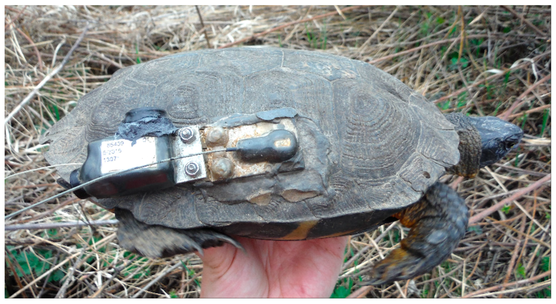
We deployed GPS units on 29 wood turtles. Nine wood turtles were only tracked in 2015, 17 were tracked in both 2015 and 2016, and three additional turtles were tracked in 2016. Nineteen of the turtles were adult females, and 10 were adult males. We removed turtles from the field for <24 h to epoxy (EP-7, Protective Coating Company, Allentown, PA, USA) a plated VHF telemetry unit (R1680, Advanced Telemetry Systems, Inc.) to the right first or second costal scute of the turtle (
Figure 1). We did not place the unit on the top of the carapace to avoid impeding the mounting of females by males during mating and to allow movement in tight spaces [
40]. Sampling and handling methods were approved by the University of Minnesota Institutional Animal Care and Use Committee (Protocol No. 1504-32514A) and permitted by the Minnesota Department of Natural Resources.
We attached the G10 UltraLITE GPS receiver and a Thermochron iButton (DS1922L; Maxim Integrated, Dallas, TX, USA) to posts on the metal plate with nuts. The iButton was coated in Plasti Dip (Plasti Dip International, Blaine, MN) to protect it from weathering and water [
41]. The weight of all three devices and epoxy was 38 g, which was <5% of the body weight for every turtle used in the study [
42,
43]. The plated VHF unit remained attached to the turtle’s carapace until removal in late summer 2016. Wood turtle GPS units and temperature loggers recorded data at the same rate as stationary tests, every 10 min. We recaptured turtles approximately every 30 days to download data and replace GPS and iButton devices. We collected wood turtle GPS data from 24 May 2015 to 19 October 2015 and 30 April 2016 to 28 August 2016. We obtained temperature data from 23 wood turtles, 16 female and 7 male, with corresponding GPS locations from 16 June 2015 to 17 July 2015 and 5 May 2016 to 28 August 2016.
To track ambient conditions, we deployed environmental temperature loggers (iButtons and Onset HOBO Pendant G receivers, model UA-004-64; Bourne, MA, USA) in aquatic and terrestrial habitats throughout the study area. All environmental temperature loggers were within 9 km of all turtles with temperature loggers. All ambient temperature iButton receivers were coated in Plasti Dip to replicate turtle deployment conditions. We recorded Twater at four water locations (including a vernal pool in 2016), Tshade at three shaded locations, and Tsun at seven open locations from May to September 2015 and 2016, at 10-minute intervals. Temperature loggers were not concurrently active at all 14 locations for the entire period.
2.6. Wood Turtle Data Analysis
We calculated FSR for all wood turtle GPS deployments and compared overall mean FSR between male and female wood turtles with a t-test assuming equal variances. We also calculated monthly FSR. The final stationary test GPS screening and moving average calculations were applied to all wood turtle GPS locations (hereafter referred to as final GPS location). We then calculated net displacement between the original and final wood turtle GPS locations. We also calculated net daily movement for each turtle by subtracting the mean x location and the mean y location for a day from the next day’s mean x and mean y location and using the Pythagorean theorem. For the wood turtle GPS locations, we also identified if the cover type changed from original to final wood turtle locations.
We created shade (T
shade), sun (T
sun), and water (T
water) temperatures by averaging simultaneous temperature readings across all sampling sites in the same environment. Temperature differences within each set of shade, sun, or water temperature loggers were minimal with the SE for T
shade, T
sun, and T
water, equal to 0.03 °C, 0.03 °C, and 0.01 °C, respectively [
44]. We included both T
shade and T
sun because 47% of the time T
sun and T
shade were separated by >1 °C. We then matched environmental temperatures and wood turtle temperature (T
turtle) to the closest 10-minute wood turtle GPS locations.
We assigned each 10-minute turtle GPS location to be on land or in water using the steps in
Table A1 following three general observations. First, a GPS location cannot be obtained when the GPS antenna is submerged in water. Second, cloacal temperatures of turtles are correlated with ambient environmental temperatures (mean difference = 0.2 °C) [
45], and internal cloacal temperature and external shell temperature are similar [
22]. Third, the temperature of water varies less throughout the day (mean T
water SD = 3.5
°C/day) than the temperature on land (mean T
shade SD = 5.3
°C/day and mean T
sun SD = 6.9
°C/day). The steps were implemented in Microsoft Excel 2010 (Microsoft Corporation, Redmond, Washington, WA, USA).
Next, we aggregated the 10-minute land or water classifications to hourly classifications because 23 percent (54,689 turtle GPS locations) were unknown. For each hour of the day, if >50% of the locations in that hour were on land, we assigned land, and if >50% of locations in that hour were in water, we assigned water. If 50% of locations were on land and 50% of locations were in water, or if >70% of locations were unknown then we initially assigned unknown to the hourly classification. If the hour before and the hour after were both classified as on land, the hour was assigned land. If the hour before and the hour after were both classified in water, the hour was assigned water. If one of the adjacent hours was classified as on land, and the other adjacent hour was classified as in water, we assigned the location type which was closest in temperature (mean Tturtle for that hour compared to mean Tshade, Tsun, and Twater for that hour). For all hours that were still classified as unknown after these assignment procedures were implemented, we then created graphs to view the temperature profile of Tshade, Tsun, Twater, and Tturtle before, during, and after the unknown hour. If a pattern was present indicating the turtle was in either water or land, we assigned that location manually. We report the overall and monthly percentage of classifiable time spent on land averaged across all, female, and male turtles.
3. Results
3.1. Stationary Tests
We obtained 16,918 GPS locations from 29 stationary test deployments. Overall mean location error (LE) for stationary test locations was 27 m (SD = 38) (
Table 1). Cover type, horizontal dilution of precision (HDOP), overhead obstruction, and time of day were included in the best model to describe LE (
Table 2). Pre-processing mean LE was 18, 29, 29, and 32 m in the open, deciduous forest, evergreen forest, and woody wetlands cover types, respectively (
Table 1). Post hoc comparisons of LE between all four cover types were significantly different (
P < 0.001), with the exception of woody wetlands and evergreen forest (
P = 0.998). The top-ranked model predicted mean LE would increase by 2 m for a unit increase in HDOP. Mean HDOP for all GPS stationary test locations was 1.28, with a range of 0.7 to 5.6. For the 16,918 GPS locations, 98.3%, 1.4%, 0.2%, and 0.05% of locations had HDOP ≤2, ≤3, ≤4, and ≤5, respectively. Overhead obstruction increased pre-processing mean LE from 25 m to 29 m (
P < 0.001). The top-ranked model identified time of day as statistically significant, but the effect was probably not of biological significance. For example, this model predicted mean LE to increase by only 1 m at mid-day in comparison to all three other time periods. The second-best model included time since deployment, with predicted decrease in mean LE of 0.04 m 12 h after deployment.
Overall, FSR for all tests was 70% (SD = 21;
Table 1). Cover type, overhead obstruction, time since deployment, and time of day were included in the best model to describe FSR (
Table 2). Post hoc comparisons of FSR between all four cover types were significantly different (
P < 0.001). FSR was 88%, 73%, 69%, and 58% in the open, deciduous forest, evergreen forest, and woody wetland cover types, respectively. FSR was 78% without an overhead obstruction and 64% with an overhead obstruction present (
P < 0.001). Our top-ranked model predicted a fix was 4.6 times more likely if a GPS receiver was not located under an overhead obstruction. The probability of a successful fix increased by a factor of 1.015 twelve hours after deployment. FSR was 67%, 69%, 72%, and 74% for morning, mid-day, evening, and night, respectively. Post hoc comparisons between time periods were significant (
P < 0.007), except for between morning and mid-day (
P = 0.130). Our top-ranked model estimated a fix was 9%, 25%, and 35% more likely to occur during mid-day, evening, or the night, compared to the morning.
The mean angle of dispersion for all GPS stationary test locations was not significant (mean angle = 89°, z = 0.99, P > 0.05). It was slightly biased for GPS locations in each cover type, but the magnitude (r) was small for all sites (range 0.02–0.12) and not biologically significant. The deciduous forest stationary test site with overhead obstruction (mean angle = 88°, z = 4.21, P < 0.05), the evergreen forest site with overhead obstruction (mean angle = 24°, z = 6.68, P < 0.05), the open site with overhead obstruction (mean angle = 175°, z = 5.46, P < 0.05), and the open site with no overhead obstruction (mean angle = 24°, z = 7.75, P < 0.001) had a slight angular bias.
3.2. GPS Outliers and Moving Averages
Mean LE in stationary tests declined from 27 to 20 m with the removal of outlier locations >60 m from the mean x and y coordinates calculated from a moving window of four locations before and four locations after. Outliers >60 m represented 9% of all locations. Removing outliers reduced LE from 18 to 15 m, 29 to 21 m, 28 to 21 m, and 33 to 24 m in open, deciduous forest, evergreen forest, and woody wetland cover types, respectively, and outliers that were removed comprised 3%, 10%, 10%, and 14% of location attempts. In the sensitivity analysis, mean LE and percent of outlying locations removed was similar whether 4, 6, 8, or 10 locations were included in the moving window (
Figure 2).
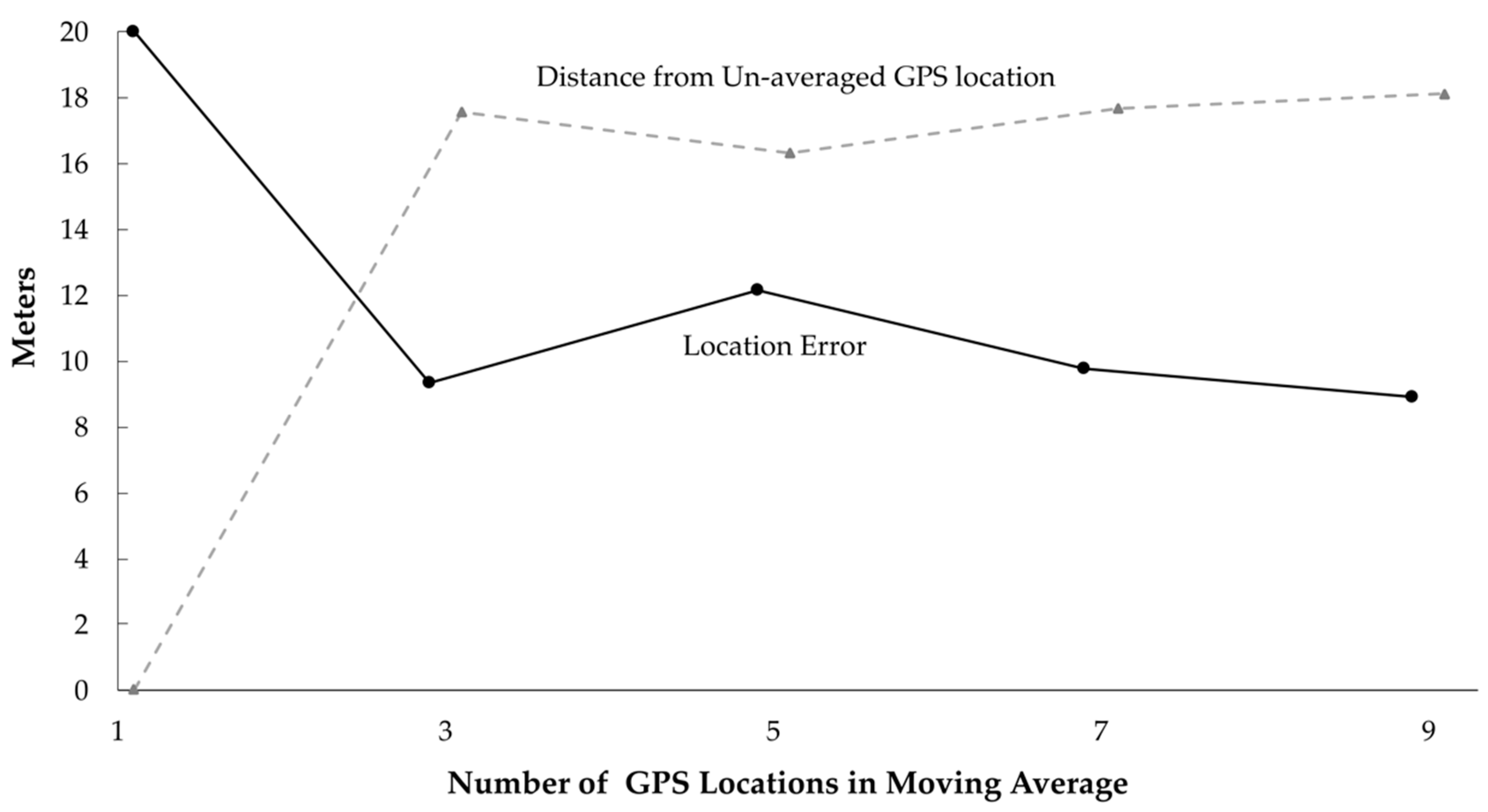
Mean LE for stationary tests was further reduced from 20 to 10 m when moving averages of up to nine total locations were applied to each screened GPS location. LE was reduced similarly in all cover types. Only four percent of locations could not be averaged with at least one other location because they were >60 min from other locations. The sensitivity analysis showed that a moving average of 3, 5, 7, and 9 adjacent GPS locations reduced mean LE to 9, 12, 10, and 9 m, respectively (
Figure 3). The distance between the original location and the final location (i.e., after screening and averaging) was 18 m (SD = 11) and did not vary with the number of locations averaged (
Figure 3).
Overall, after removing outlier locations and applying moving averages, we reduced mean LE for all stationary tests from 27 to 10 m. We reduced 50% circular error probable from 19 to 8 m, and 95% circular error probable from 74 to 24 m.
3.3. Wood Turtle GPS and Temperature Data
Overall FSR when GPS units were deployed on wood turtles was 26%, with 122,657 GPS locations obtained in 464,415 location attempts (mean = 61,328 locations/turtle, SD = 26,508). This included a total of 3748 turtle days with GPS data (mean = 150 days/turtle, SD = 76). The FSR for all location attempts when turtles were on land was 38% (SD = 9). Mean FSR for all turtle land locations was 56%, 36%, 34%, and 34% in May, June, July, and August, respectively. Overall FSR was not different between male and female wood turtles (t-test, t18 = 2.10, P = 0.385).
The GPS units had missing data or failed to record any data on 22% of all 30-day deployments due to battery failure, programming errors, or unknown causes. Mean HDOP for turtle GPS locations was 1.35 (SD = 0.34, range = 0.7–36.2). Only 73 of the 122,657 total wood turtle GPS locations were discarded because HDOP was >5. Approximately 12% of turtle GPS locations were outliers >60 m from the mean location of a moving window before and after a given GPS location. After removing the outlier location, 84% of turtle GPS locations could be averaged in a 7-location moving window. We did not calculate other moving window sizes for turtle data because in stationary tests moving windows of 3, 5, 7, and 9 were similar (
Figure 3). The moving window averaging displaced turtle GPS locations a mean of 18 m (SD = 12). This displacement changed the cover type for 19% of turtle locations, but the net change of cover types was <1%.
Net movement/day by females varied because of movements during the nesting period. The highest net daily movements were between May 21 and June 29 (
Figure 4). During the nesting period, female average net movement/day was 128 m (SD = 20), while at other times of the year the average net movement/day for females was 52 m (SD = 43). In contrast, males had an average net movement/day of 48 m (SD = 68), which was relatively constant throughout the summer. The largest net movement/day was 6.21 km for a female wood turtle and 0.97 km for a male wood turtle. About 70% of the net movements per day were <50 m for both female and male wood turtles.
We collected 399,606 temperatures at a 10-minute interval from the temperature loggers attached to 23 turtles (mean = 15,369 readings/turtle, SD = 7179), of which 242,781 readings corresponded to times in which a turtle’s GPS receiver was active. Temperature devices did not read data on 22% of all deployments. The initial rules (
Table A1) used to classify each 10-minute location to be on land or in water classified 53%, 25%, and 23% of locations in land, water, or unknown, respectively. We then aggregated all 242,781 locations into hourly intervals, resulting in 40,532 land, water, or unknown designations. Of these hourly locations, 83% were defined as on land or in water based on our two-step automated procedure, 14% were manually defined, and 3% of locations remained unknown.
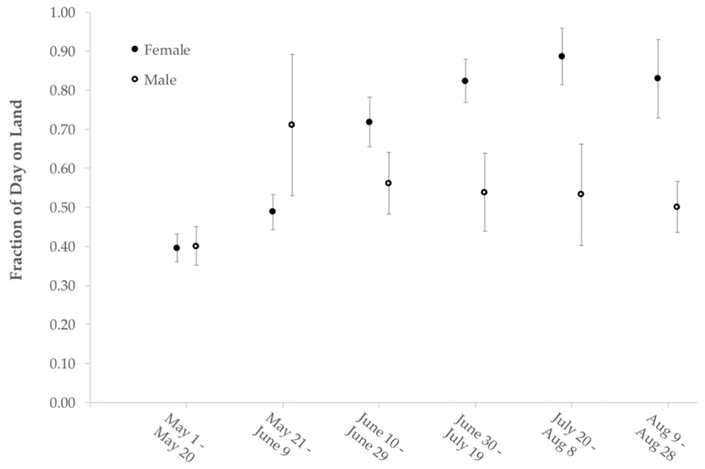
Turtles spent on average 68% (SD = 12) of time on land and 32% (SD = 12) of time in water from mid-May to late-August in 2015 and 2016. The percentage of time spent on land for all turtles was 48% (SD =10), 66% (SD = 12), 75% (SD = 18), and 67% (SD =19) in May, June, July, and August, respectively. Female wood turtles spent 45% (SD = 8), 69% (SD = 11), 85% (SD = 8), and 78% (SD = 15) of time on land in May, June, July, and August in comparison to 54% (SD = 11), 56% (SD = 9), 54% (SD = 14), and 48% (SD = 7) for male wood turtles (
Figure 5).
4. Discussion
We used stationary tests to better understand the accuracy of snapshot GPS locations and to search for possible sources of bias specific to the habitat and behavior of semi-aquatic turtles in northeastern Minnesota. Using stationary test locations enabled us to identify the most influential rule in reducing LE, removing locations outside of an average x and y coordinate calculated from a moving average of surrounding locations. Removing outlier locations is an important first step in preparing GPS locations for analysis [
37]. The outlier threshold will vary depending on GPS unit and study species, which is why we used a sensitivity analysis to identify the trade-off between data loss and spatial error. Our 60 m outlier threshold resulted in a 10% data loss but increased mean accuracy by 7 m.
An important aspect of ecology in wood turtles and other semi-aquatic turtles (e.g., spotted turtles [
Clemmys guttata]) [
46], is that they are relatively sedentary on land over short periods. Slow movement rates combined with frequent (10-minute) GPS intervals improved positional accuracy using moving averages. Using the stationary GPS locations, a moving average decreased mean location error from 20 to 10 m. Final mean location error was similar whether 3, 5, 7, or 9 adjacent locations were averaged and the mean distance a GPS location was adjusted was 18 m. The larger memory capacity and battery life of miniaturized GPS units make this moving average approach feasible for GPS studies involving semi-aquatic turtles.
Combining GPS data with a temperature logger is advantageous for quantifying semi-aquatic turtle habitat selection because it can take advantage of the fact that GPS signals do not penetrate water. This approach is similar to using a light sensor to determine when an animal is in a burrow [
2]. Building on previous work describing the thermal biology of turtles via temperature dataloggers [
22,
24], we were able to specify if water or terrestrial habitat obstruction was the cause of unsuccessful GPS fixes. Instead of an overall FSR of 27%, similar to the Blanding’s turtle [
4], we were able to identify FSR in largely forested habitats to be 38%.
Not surprisingly, cover type and the presence of an overhead obstruction had the largest effect of all covariates on the ability of GPS units to attain accurate fixes. Habitats under woody or herbaceous vegetation had reduced LE and FSR in comparison to open sites. We also identified several covariates that had significance to describe LE and FSR, but not biological significance. For example, time since deployment did not have a significant impact on mean LE as the probability of a successful fix increased by only 3% one day after deployment. A difference in mean LE of <7 m and a difference in FSR of <7% between different times of day is small enough that it would be unlikely to affect inferences about turtle behavior relative to other factors. However, the fact that GPS locations were more easily attained at night in our study area suggests that GPS units could prove to be especially useful for tracking nighttime movements, which is particularly challenging with VHF tracking. While other studies have demonstrated how the removal of locations with high horizontal dilution of precision (HDOP) values reduces LE, this screening procedure was not effective at reducing overall LE in our study due to low average HDOP values for all tests. The snapshot GPS unit software only calculated locations with ≥6 satellites and, thus, only 2% of locations had HDOP >2. GPS studies that do not include snapshot technology should still consider HDOP an important covariate to describe LE and FSR.
Our study provides a foundation to understand the benefits and challenges inherent in freshwater turtle GPS telemetry. We developed methods to process snapshot GPS locations and reduce location error to ca. 10 m. The moving average method can be used if the location interval is short and the study animal is relatively sedentary. Based on our analyses, we recommend that analyses of terrestrial habitat use consider missing GPS locations that are biased against densely covered areas. In species such as the wood turtle that do not move very quickly, biologists could consider extrapolating missing locations based on the movement paths of an animal before and after it enters forested habitat. Otherwise, resource selection analyses should account for these missing values. Despite the challenges to GPS data in semi-aquatic species, our snapshot GPS units collected almost 150,000 wood turtle GPS locations. Our systematic approach to enhance GPS data accuracy provides a foundation for future semi-aquatic turtle movement and habitat analyses. Future studies should consider GPS units for similar freshwater turtles if researchers cannot commit to time-intensive VHF-tracking or there is a need for a large spatial dataset that includes locations across all times of day and night. These data will provide a foundation for future research on diel movement patterns and habitat preferences.


