
Explainability of Protein Deep Learning Models


Abstract
1. Introduction and Background
1.1. Protein Embeddings
1.2. Protein Interaction-Site Prediction
1.3. Explainable AI (XAI) Methods
1.4. Explaining Protein Learning Models
2. Results and Discussion
2.1. Data
2.2. Comparison with Random Matrices
2.3. Amino Acid Properties
2.4. Comparison of Amino Acid Properties
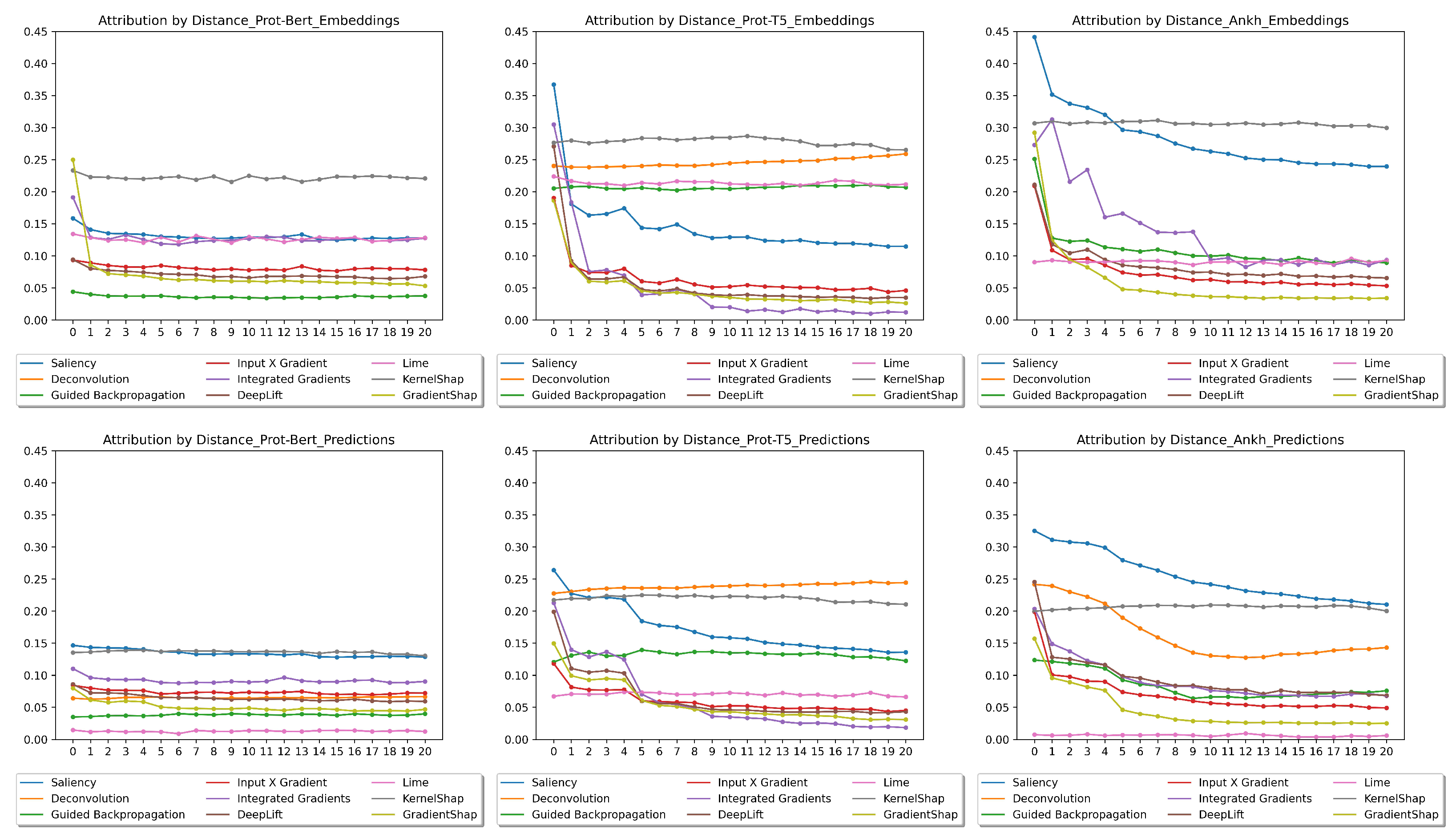
2.5. Distances
2.6. Infidelity
3. Materials and Methods
3.1. Interpretability of Protein Embeddings
3.2. Interpretability of Interaction-Site Prediction Models
3.3. Evaluation of Interpretations
3.3.1. Categorical Tests
- 1.
- Interacting and non-interacting amino acids.
- 2.
- Aromatic and non-aromatic amino acids.
- 3.
- Acidic and basic amino acids.
3.3.2. Numerical Tests
3.3.3. Distance
3.3.4. Explanation Infidelity
3.4. Implementation
4. Conclusions
Author Contributions
Funding
Data Availability Statement
Acknowledgments
Conflicts of Interest
References
- Jumper, J.; Evans, R.; Pritzel, A.; Green, T.; Figurnov, M.; Ronneberger, O.; Tunyasuvunakool, K.; Bates, R.; Žídek, A.; Potapenko, A.; et al. Highly accurate protein structure prediction with AlphaFold. Nature 2021, 596, 583–589. [Google Scholar] [CrossRef] [PubMed]
- Baek, M.; DiMaio, F.; Anishchenko, I.; Dauparas, J.; Ovchinnikov, S.; Lee, G.; Wang, J.; Cong, Q.; Kinch, L.; Schaeffer, R.; et al. Accurate prediction of protein structures and interactions using a three-track neural network. Science 2021, 373, eabj8754. [Google Scholar] [CrossRef] [PubMed]
- Alley, E.; Khimulya, G.; Biswas, S.; Alquraishi, M.; Church, G. Unified rational protein engineering with sequence-based deep representation learning. Nat. Methods 2019, 16, 1315–1322. [Google Scholar] [CrossRef] [PubMed]
- Elnaggar, A.; Heinzinger, M.; Dallago, C.; Rehawi, G.; Yu, W.; Jones, L.; Gibbs, T.; Feher, T.; Angerer, C.; Steinegger, M.; et al. ProtTrans: Towards Cracking the Language of Lifes Code Through Self-Supervised Deep Learning and High Performance Computing. IEEE Trans. Pattern Anal. Mach. Intell. 2021, 44, 7112–7127. [Google Scholar] [CrossRef]
- Strokach, A.; Becerra, D.; Corbi-Verge, C.; Perez-Riba, A.; Kim, P. Fast and Flexible Protein Design Using Deep Graph Neural Networks. Cell Syst. 2020, 11, 402–411. [Google Scholar] [CrossRef]
- Anishchenko, I.V.; Pellock, S.J.; Chidyausiku, T.M.; Ramelot, T.A.; Ovchinnikov, S.; Hao, J.; Bafna, K.; Norn, C.H.; Kang, A.; Bera, A.K.; et al. De novo protein design by deep network hallucination. Nature 2020, 600, 547–552. [Google Scholar] [CrossRef]
- Trinquier, J.; Uguzzoni, G.; Pagnani, A.; Zamponi, F.; Weigt, M. Efficient generative modeling of protein sequences using simple autoregressive models. Nat. Commun. 2021, 12, 5800. [Google Scholar] [CrossRef]
- Mikolov, T.; Sutskever, I.; Chen, K.; Corrado, G.; Dean, J. Distributed Representations of Words and Phrases and their Compositionality. Adv. Neural Inf. Process. Syst. 2013, 26. [Google Scholar]
- Pennington, J.; Socher, R.; Manning, C. GloVe: Global Vectors for Word Representation. In Proceedings of the 2014 Conference on Empirical Methods in Natural Language Processing (EMNLP); Moschitti, A., Pang, B., Daelemans, W., Eds.; Association for Computational Linguistics: Minneapolis, MN, USA, 2014; pp. 1532–1543. [Google Scholar] [CrossRef]
- Devlin, J.; Chang, M.W.; Lee, K.; Toutanova, K. BERT: Pre-training of Deep Bidirectional Transformers for Language Understanding. In Proceedings of the North American Chapter of the Association for Computational Linguistics; Association for Computational Linguistics: Minneapolis, MN, USA, 2019. [Google Scholar]
- Raffel, C.; Shazeer, N.M.; Roberts, A.; Lee, K.; Narang, S.; Matena, M.; Zhou, Y.; Li, W.; Liu, P.J. Exploring the Limits of Transfer Learning with a Unified Text-to-Text Transformer. J. Mach. Learn. Res. 2019, 21, 140:1–140:67. [Google Scholar]
- Asgari, E.; Mofrad, M.R.K. ProtVec: A Continuous Distributed Representation of Biological Sequences. arXiv 2015, arXiv:1503.05140. [Google Scholar]
- Heinzinger, M.; Elnaggar, A.; Wang, Y.; Dallago, C.; Nechaev, D.; Matthes, F.; Rost, B. Modeling aspects of the language of life through transfer-learning protein sequences. BMC Bioinform. 2019, 20, 723. [Google Scholar] [CrossRef] [PubMed]
- Bepler, T.; Berger, B. Learning protein sequence embeddings using information from structure. arXiv 2019, arXiv:1902.08661. [Google Scholar]
- Rao, R.; Liu, J.; Verkuil, R.; Meier, J.; Canny, J.F.; Abbeel, P.; Sercu, T.; Rives, A. MSA Transformer. biorXiv 2021.
- Rives, A.; Meier, J.; Sercu, T.; Goyal, S.; Lin, Z.; Liu, J.; Guo, D.; Ott, M.; Zitnick, C.L.; Ma, J.; et al. Biological structure and function emerge from scaling unsupervised learning to 250 million protein sequences. Proc. Natl. Acad. Sci. USA 2021, 118, e2016239118. [Google Scholar] [CrossRef] [PubMed]
- Elnaggar, A.; Essam, H.; Salah-Eldin, W.; Moustafa, W.; Elkerdawy, M.; Rochereau, C.; Rost, B. Ankh: Optimized protein language model unlocks general-purpose modelling. arXiv 2023, arXiv:2301.06568. [Google Scholar]
- Yuan, Q.; Chen, J.; Zhao, H.; Zhou, Y.; Yang, Y. Structure-aware protein-protein interaction site prediction using deep graph convolutional network. Bioinformatics 2021, 38, 125–132. [Google Scholar] [CrossRef]
- Zeng, M.; Zhang, F.; Wu, F.X.; Li, Y.; Wang, J.; Li, M. Protein-protein interaction site prediction through combining local and global features with deep neural networks. Bioinformatics 2019, 36, 1114–1120. [Google Scholar] [CrossRef]
- Zhang, B.; Li, J.; Quan, L.; Chen, Y.; Lü, Q. Sequence-based prediction of protein-protein interaction sites by simplified long-short term memory network. Neurocomputing 2019, 357, 86–100. [Google Scholar] [CrossRef]
- Li, Y.; Golding, G.; Ilie, L. DELPHI: Accurate deep ensemble model for protein interaction sites prediction. Bioinformatics 2020, 37, 896–904. [Google Scholar] [CrossRef]
- Hosseini, S.; Ilie, L. PITHIA: Protein Interaction Site Prediction Using Multiple Sequence Alignments and Attention. Int. J. Mol. Sci. 2022, 23, 12814. [Google Scholar] [CrossRef]
- Manfredi, M.; Savojardo, C.; Martelli, P.L.; Casadio, R. ISPRED-SEQ: Deep neural networks and embeddings for predicting interaction sites in protein sequences. J. Mol. Biol. 2023, 435, 167963. [Google Scholar] [CrossRef] [PubMed]
- Hosseini, S.; Golding, G.B.; Ilie, L. Seq-InSite: Sequence supersedes structure for protein interaction site prediction. Bioinformatics 2024, 40, btad738. [Google Scholar] [CrossRef] [PubMed]
- Molnar, C. Interpretable Machine Learning, 2nd ed.; Independently Published, 2022. [Google Scholar]
- Simonyan, K.; Vedaldi, A.; Zisserman, A. Deep Inside Convolutional Networks: Visualising Image Classification Models and Saliency Maps. arXiv 2013, arXiv:1312.6034. [Google Scholar]
- Zeiler, M.D.; Fergus, R. Visualizing and Understanding Convolutional Networks. In Lecture Notes in Computer Science, Proceedings of the Computer Vision–ECCV 2014–13th European Conference, Zurich, Switzerland, 6–12 September 2014; Fleet, D.J., Pajdla, T., Schiele, B., Tuytelaars, T., Eds.; Springer: Berlin/Heidelberg, Germany, 2014; Volume 8689, pp. 818–833. [Google Scholar] [CrossRef]
- Springenberg, J.T.; Dosovitskiy, A.; Brox, T.; Riedmiller, M.A. Striving for Simplicity: The All Convolutional Net. arXiv 2014, arXiv:1412.6806. [Google Scholar]
- Shrikumar, A.; Greenside, P.; Shcherbina, A.; Kundaje, A. Not Just a Black Box: Learning Important Features Through Propagating Activation Differences. arXiv 2016, arXiv:1605.01713. [Google Scholar]
- Ancona, M.; Ceolini, E.; Öztireli, C.; Gross, M. Towards better understanding of gradient-based attribution methods for Deep Neural Networks. In Proceedings of the 6th International Conference on Learning Representations, ICLR 2018, Vancouver, BC, Canada, 30 April–3 May 2018; Conference Track Proceedings; OpenReview.net. 2018. [Google Scholar]
- Shrikumar, A.; Greenside, P.; Kundaje, A. Learning Important Features Through Propagating Activation Differences. arXiv 2017, arXiv:1704.02685. [Google Scholar]
- Sundararajan, M.; Taly, A.; Yan, Q. Axiomatic Attribution for Deep Networks. In Machine Learning Research, Proceedings of the 34th International Conference on Machine Learning, ICML 2017, Sydney, NSW, Australia, 6–11 August 2017; Precup, D., Teh, Y.W., Eds.; PMLR: Cambridge, MA, USA, 2017; Volume 70, pp. 3319–3328. [Google Scholar]
- Ribeiro, M.T.; Singh, S.; Guestrin, C. “Why Should I Trust You?”: Explaining the Predictions of Any Classifier. In Proceedings of the Demonstrations Session, NAACL HLT 2016, the 2016 Conference of the North American Chapter of the Association for Computational Linguistics: Human Language Technologies, San Diego, CA, USA, 12–17 June 2016; The Association for Computational Linguistics: Stroudsburg, PA, USA, 2016; pp. 97–101. [Google Scholar] [CrossRef]
- Lundberg, S.M.; Lee, S. A unified approach to interpreting model predictions. arXiv 2017, arXiv:1705.07874. [Google Scholar]
- Kokhlikyan, N.; Miglani, V.; Martin, M.; Wang, E.; Alsallakh, B.; Reynolds, J.; Melnikov, A.; Kliushkina, N.; Araya, C.; Yan, S.; et al. Captum: A unified and generic model interpretability library for PyTorch. arXiv 2020, arXiv:2009.07896. [Google Scholar]
- Ali, A.; Schnake, T.; Eberle, O.; Montavon, G.; Müller, K.R.; Wolf, L. XAI for Transformers: Better Explanations through Conservative Propagation. In Machine Learning Research, Proceedings of the 39th International Conference on Machine Learning, Baltimore, MD, USA, 17–23 July 2022; Chaudhuri, K., Jegelka, S., Song, L., Szepesvari, C., Niu, G., Sabato, S., Eds.; PMLR: Cambridge, MA, USA, 2022; Volume 162, pp. 435–451. [Google Scholar]
- Chefer, H.; Gur, S.; Wolf, L. Transformer Interpretability Beyond Attention Visualization. In Proceedings of the IEEE/CVF Conference on Computer Vision and Pattern Recognition (CVPR), Nashville, TN, USA, 20–25 June 2021; pp. 782–791. [Google Scholar]
- Mohebbi, H.; Jumelet, J.; Hanna, M.; Alishahi, A.; Zuidema, W. Transformer-specific Interpretability. In Proceedings of the 18th Conference of the European Chapter of the Association for Computational Linguistics: Tutorial Abstracts; Mesgar, M., Loáiciga, S., Eds.; Association for Computational Linguistics: Stroudsburg, PA, USA, 2024; pp. 21–26. [Google Scholar]
- Fantozzi, P.; Naldi, M. The Explainability of Transformers: Current Status and Directions. Computers 2024, 13, 92. [Google Scholar] [CrossRef]
- Allison, L.A. Fundamental Molecular Biology, 2nd ed.; Wiley: Hoboken, NJ, USA, 2012. [Google Scholar]
- Weast, R. CRC Handbook of Chemistry and Physics, 62nd ed.; CRC Press: Boca Raton, FL, USA, 1981. [Google Scholar]
- Mann, H.B.; Whitney, D.R. On a Test of Whether one of Two Random Variables is Stochastically Larger than the Other. Ann. Math. Stat. 1947, 18, 50–60. [Google Scholar] [CrossRef]
- Yeh, C.K.; Hsieh, C.Y.; Suggala, A.S.; Inouye, D.I.; Ravikumar, P. On the (In)fidelity and Sensitivity of Explanations. In Proceedings of the Neural Information Processing Systems, Vancouver, BC, Canada, 8–14 December 2019. [Google Scholar]
- Wolf, T.; Debut, L.; Sanh, V.; Chaumond, J.; Delangue, C.; Moi, A.; Cistac, P.; Rault, T.; Louf, R.; Funtowicz, M.; et al. Transformers: State-of-the-Art Natural Language Processing. In Proceedings of the 2020 Conference on Empirical Methods in Natural Language Processing: System Demonstrations, Online, 16–20 November 2020; Association for Computational Linguistics (ACL): Stroudsburg, PA, USA, 2020; pp. 38–45. [Google Scholar]
- Ansel, J.; Yang, E.; He, H.; Gimelshein, N.; Jain, A.; Voznesensky, M.; Bao, B.; Bell, P.; Berard, D.; Burovski, E.; et al. PyTorch 2: Faster Machine Learning Through Dynamic Python Bytecode Transformation and Graph Compilation. In Proceedings of the 29th ACM International Conference on Architectural Support for Programming Languages and Operating Systems, La Jolla, CA, USA, 27 April–1 May 2024; Volume 2. [Google Scholar]

| Protein ID | Chain | Length | Protein ID | Chain | Length |
|---|---|---|---|---|---|
| 2CCI | F | 30 | 1SGH | B | 39 |
| 1MZW | B | 31 | 6F4U | D | 40 |
| 1OQE | K | 31 | 2L9U | A | 40 |
| 5KQ1 | C | 31 | 5OM2 | B | 40 |
| 5JPO | E | 32 | 2XZE | R | 40 |
| 2L34 | A | 33 | 4LZX | B | 40 |
| 6B7G | B | 33 | 5TUV | C | 41 |
| 3MJH | B | 34 | 2XA6 | A | 41 |
| 4NAW | D | 34 | 2MOF | A | 42 |
| 3DXC | B | 35 | 2K9J | B | 43 |
| 2XJY | B | 35 | 2F9D | P | 43 |
| 2BE6 | D | 37 | 4GDO | A | 43 |
| 1IK9 | C | 37 | 6GNY | B | 43 |
| 5XJL | M | 37 | 6AU8 | C | 43 |
| 5FV8 | E | 38 | 2KS1 | A | 44 |
| 4UED | B | 38 | 3HRO | A | 44 |
| 5FV8 | A | 38 | 2L2T | A | 44 |
| Amino Acid | Hydrophobicity | Molecular Mass | Van der Waals Volume | Dipole Moment | Aromaticity | Acidity/Basicity |
|---|---|---|---|---|---|---|
| Glycine (G) | −0.4 | 57 | 48 | 0.000 | ||
| Alanine (A) | 1.8 | 71 | 67 | 5.937 | ||
| Serine (S) | −0.8 | 87 | 73 | 9.836 | ||
| Proline (P) | −1.6 | 97 | 90 | 7.916 | ||
| Valine (V) | 4.2 | 99 | 105 | 2.692 | ||
| Threonine (T) | −0.7 | 101 | 93 | 9.304 | ||
| Cysteine (C) | 2.5 | 103 | 86 | 10.740 | ||
| Isoleucine (I) | 4.5 | 113 | 124 | 3.371 | ||
| Leucine (L) | 3.8 | 113 | 124 | 3.782 | ||
| Asparagine (N) | −3.5 | 114 | 96 | 18.890 | ||
| Aspartic acid (D) | −3.5 | 115 | 91 | 29.490 | A | |
| Glutamine (Q) | −3.5 | 128 | 114 | 39.890 | ||
| Lysine (K) | −3.9 | 128 | 135 | 50.020 | B | |
| Glutamic acid (E) | −3.5 | 129 | 109 | 42.520 | A | |
| Methionine (M) | 1.9 | 131 | 124 | 8.589 | ||
| Histidine (H) | −3.2 | 137 | 118 | 20.440 | B | |
| Phenylalanine (F) | 2.8 | 147 | 135 | 5.980 | A | |
| Arginine (R) | −4.5 | 156 | 148 | 37.500 | B | |
| Tyrosine (Y) | −1.3 | 163 | 141 | 10.410 | A | |
| Tryptophan (W) | −0.9 | 186 | 163 | 10.730 | A |
| Method | Interactivity | Aromaticity | Acidity/Basicity | Interactivity | Aromaticity | Acidity/Basicity |
|---|---|---|---|---|---|---|
| Embeddings—Target | Embeddings—Source | |||||
| Saliency | 6.09 × 10⁻²⁸ | 1.87 × 10−82 | 8.98 × 10⁻³¹ | 1.88 × 10⁻²¹ | 1.21 × 10−124 | 7.03 × 10⁻²² |
| Deconvolution | 5.05 × 10⁻¹ | 2.83 × 10⁻¹ | 2.79 × 10⁻¹ | 4.71 × 10⁻² | 1.53 × 10⁻⁴ | 2.55 × 10⁻¹ |
| Guided Backprop. | 5.05 × 10⁻¹ | 2.83 × 10⁻¹ | 2.79 × 10⁻¹ | 4.71 × 10⁻² | 1.53 × 10⁻⁴ | 2.55 × 10⁻¹ |
| Input X Grad. | 6.16 × 10⁻² | 6.45 × 10⁻¹ | 6.98 × 10⁻¹ | 2.41 × 10⁻² | 1.86 × 10⁻² | 1.60 × 10⁻¹ |
| DeepLIFT | 4.56 × 10⁻¹ | 3.48 × 10⁻¹ | 1.47 × 10⁻² | 3.28 × 10⁻¹ | 1.62 × 10⁻³ | 2.15 × 10⁻² |
| Integrated Grad. | 5.09 × 10⁻¹ | 9.09 × 10⁻² | 1.20 × 10⁻⁸ | 2.28 × 10⁻¹⁹ | 1.09 × 10⁻⁵ | 2.92 × 10⁻¹⁹ |
| LIME | 3.82 × 10⁻¹ | 5.47 × 10⁻¹ | 3.93 × 10⁻¹ | 6.28 × 10⁻¹ | 3.55 × 10⁻¹ | 2.24 × 10⁻¹ |
| KernelShap | 0.00 × 100 | 3.74 × 10−126 | 2.41 × 10⁻²⁰ | 3.95 × 10⁻³³ | 7.09 × 10⁻¹⁷ | 1.01 × 10⁻¹² |
| GradientShap | 2.79 × 10⁻¹ | 9.32 × 10⁻¹ | 8.37 × 10⁻⁶ | 6.14 × 10⁻¹ | 2.35 × 10⁻² | 7.30 × 10⁻¹ |
| Predictions—Target | Predictions—Source | |||||
| Saliency | 6.20 × 10−52 | 1.04 × 10−170 | 4.58 × 10−38 | 7.43 × 10⁻² | 3.49 × 10−219 | 1.90 × 10⁻³² |
| Deconvolution | 1.65 × 10⁻² | 1.29 × 10⁻⁶ | 2.63 × 10⁻¹ | 7.41 × 10⁻¹ | 6.66 × 10⁻⁹ | 8.29 × 10⁻⁹ |
| Guided Backprop. | 6.56 × 10⁻³ | 9.32 × 10⁻¹ | 4.12 × 10⁻¹ | 2.53 × 10⁻¹ | 3.52 × 10⁻³ | 3.53 × 10⁻¹ |
| Input X Grad. | 9.01 × 10⁻¹ | 8.19 × 10⁻¹ | 7.53 × 10⁻¹ | 2.88 × 10⁻¹ | 1.46 × 10⁻² | 4.90 × 10⁻¹ |
| DeepLIFT | 7.11 × 10⁻¹³ | 4.81 × 10⁻¹ | 3.41 × 10⁻¹ | 6.81 × 10⁻⁶ | 4.63 × 10⁻⁴ | 7.06 × 10⁻² |
| Integrated Grad. | 6.86 × 10−108 | 4.81 × 10⁻¹ | 4.23 × 10⁻²⁰ | 1.51 × 10⁻² | 9.82 × 10⁻⁷ | 2.76 × 10⁻⁷ |
| LIME | 2.06 × 10⁻¹ | 7.92 × 10⁻¹ | 1.67 × 10⁻¹ | 4.45 × 10⁻¹ | 3.82 × 10⁻¹ | 1.91 × 10⁻¹ |
| KernelShap | 3.96 × 10−236 | 4.68 × 10−157 | 1.12 × 10⁻²⁰ | 2.49 × 10⁻²⁹ | 2.97 × 10⁻¹² | 1.34 × 10⁻⁷ |
| GradientShap | 2.92 × 10⁻¹ | 2.87 × 10⁻² | 4.41 × 10⁻⁵ | 9.66 × 10⁻¹ | 2.82 × 10⁻² | 8.91 × 10⁻¹ |
| Method | Interactivity | Aromaticity | Acidity/Basicity | Interactivity | Aromaticity | Acidity/Basicity |
|---|---|---|---|---|---|---|
| Embeddings—Target | Embeddings—Source | |||||
| Saliency | 2.58 × 10⁻⁹ | 5.67 × 10⁻⁸ | 8.32 × 10⁻² | 2.49 × 10−152 | 1.19 × 10⁻² | 8.39 × 10−61 |
| Deconvolution | 4.53 × 10⁻¹⁵ | 7.06 × 10⁻¹ | 2.79 × 10⁻² | 3.12 × 10⁻² | 4.96 × 10−45 | 0.00 × 100 |
| Guided Backprop. | 5.25 × 10⁻⁶ | 9.70 × 10⁻¹ | 7.20 × 10−60 | 3.57 × 10⁻¹⁴ | 1.35 × 10⁻³⁵ | 9.16 × 10−139 |
| Input X Grad. | 6.85 × 10⁻² | 7.12 × 10⁻¹ | 4.75 × 10⁻¹ | 3.25 × 10⁻¹ | 9.18 × 10⁻¹ | 3.60 × 10⁻¹ |
| DeepLIFT | 5.95 × 10⁻¹ | 3.73 × 10⁻¹ | 5.07 × 10⁻¹ | 3.82 × 10⁻²² | 8.98 × 10⁻³⁰ | 1.41 × 10⁻²¹ |
| Integrated Grad. | 2.19 × 10⁻¹ | 8.96 × 10⁻² | 8.56 × 10⁻¹ | 9.56 × 10⁻³² | 4.23 × 10⁻⁴ | 3.23 × 10⁻¹ |
| LIME | 7.64 × 10⁻¹ | 1.58 × 10⁻¹ | 7.80 × 10⁻¹ | 9.03 × 10⁻¹ | 4.18 × 10⁻¹ | 5.31 × 10⁻¹ |
| KernelShap | 1.17 × 10⁻² | 3.79 × 10−67 | 5.89 × 10−63 | 2.84 × 10⁻¹³ | 3.61 × 10⁻⁵ | 6.75 × 10⁻³ |
| GradientShap | 9.30 × 10⁻² | 7.30 × 10⁻² | 8.92 × 10⁻¹ | 7.21 × 10⁻² | 1.23 × 10⁻¹ | 4.41 × 10⁻¹ |
| Predictions—Target | Predictions—Source | |||||
| Saliency | 5.61 × 10⁻² | 1.29 × 10⁻³³ | 2.52 × 10⁻¹ | 4.48 × 10−132 | 6.03 × 10⁻¹ | 3.49 × 10−127 |
| Deconvolution | 8.16 × 10−69 | 5.95 × 10⁻¹² | 6.02 × 10⁻¹ | 1.71 × 10⁻¹⁴ | 9.20 × 10−62 | 0.00 × 100 |
| Guided Backprop. | 5.26 × 10−94 | 7.31 × 10⁻² | 8.84 × 10−102 | 9.26 × 10⁻¹² | 1.17 × 10−61 | 9.02 × 10−276 |
| Input X Grad. | 1.44 × 10⁻¹ | 4.54 × 10⁻¹ | 7.71 × 10⁻¹ | 9.88 × 10⁻¹ | 6.27 × 10⁻¹ | 7.30 × 10⁻¹ |
| DeepLIFT | 1.12 × 10⁻¹ | 1.94 × 10⁻¹ | 2.13 × 10⁻¹ | 2.27 × 10⁻¹⁹ | 1.67 × 10⁻²² | 2.37 × 10⁻¹⁸ |
| Integrated Grad. | 1.09 × 10⁻² | 8.95 × 10⁻¹ | 9.01 × 10⁻¹ | 4.77 × 10⁻²⁸ | 8.94 × 10⁻¹ | 9.82 × 10⁻¹ |
| LIME | 8.42 × 10⁻¹ | 1.42 × 10⁻¹ | 7.55 × 10⁻¹ | 6.80 × 10⁻¹ | 6.38 × 10⁻¹ | 7.21 × 10⁻¹ |
| KernelShap | 1.62 × 10−93 | 3.90 × 10⁻⁷ | 6.22 × 10⁻²¹ | 3.40 × 10⁻⁶ | 2.35 × 10⁻³ | 1.77 × 10⁻³ |
| GradientShap | 5.14 × 10⁻¹ | 7.91 × 10⁻¹ | 2.08 × 10⁻¹ | 7.09 × 10⁻² | 3.88 × 10⁻¹ | 9.76 × 10⁻¹ |
| Method | Interactivity | Aromaticity | Acidity/Basicity | Interactivity | Aromaticity | Acidity/Basicity |
|---|---|---|---|---|---|---|
| Embeddings—Target | Embeddings—Source | |||||
| Saliency | 5.59 × 10−164 | 2.64 × 10⁻⁵ | 7.14 × 10⁻² | 9.23 × 10−101 | 4.12 × 10⁻¹ | 1.81 × 10⁻¹ |
| Deconvolution | 5.00 × 10⁻³ | 8.79 × 10⁻¹ | 6.77 × 10⁻¹⁶ | 5.95 × 10⁻²² | 7.93 × 10⁻¹ | 5.57 × 10⁻⁷ |
| Guided Backprop. | 5.00 × 10⁻³ | 8.79 × 10⁻¹ | 6.77 × 10⁻¹⁶ | 5.95 × 10⁻²² | 7.93 × 10⁻¹ | 5.57 × 10⁻⁷ |
| Input X Grad. | 6.45 × 10⁻¹ | 3.69 × 10⁻³ | 6.14 × 10⁻³ | 3.01 × 10⁻¹ | 5.36 × 10⁻⁵ | 2.88 × 10⁻¹ |
| DeepLIFT | 5.75 × 10⁻⁸ | 2.57 × 10⁻¹ | 3.58 × 10⁻¹ | 1.45 × 10⁻¹ | 2.65 × 10⁻³ | 2.80 × 10⁻² |
| Integrated Grad. | 2.50 × 10⁻¹ | 3.29 × 10⁻² | 7.26 × 10⁻⁸ | 1.94 × 10⁻²⁷ | 2.51 × 10−87 | 2.12 × 10−288 |
| LIME | 2.18 × 10⁻¹ | 2.40 × 10⁻¹ | 3.04 × 10⁻¹ | 4.60 × 10⁻² | 9.19 × 10⁻² | 6.05 × 10⁻¹ |
| KernelShap | 1.78 × 10⁻²¹ | 3.01 × 10⁻³ | 0.00 × 100 | 1.61 × 10⁻⁴ | 1.54 × 10⁻⁵ | 1.04 × 10⁻¹¹ |
| GradientShap | 1.51 × 10⁻¹ | 9.62 × 10⁻¹ | 3.46 × 10⁻¹ | 5.43 × 10⁻³ | 5.03 × 10⁻³ | 2.45 × 10⁻⁵ |
| Predictions—Target | Predictions—Source | |||||
| Saliency | 0.00 × 100 | 1.70 × 10⁻²⁹ | 8.82 × 10⁻⁷ | 2.22 × 10−154 | 1.48 × 10⁻¹ | 7.43 × 10⁻⁸ |
| Deconvolution | 3.97 × 10⁻¹⁴ | 4.89 × 10⁻⁵ | 6.77 × 10⁻⁸ | 1.59 × 10⁻¹⁵ | 1.38 × 10⁻¹² | 5.22 × 10⁻¹ |
| Guided Backprop. | 5.68 × 10⁻⁶ | 9.42 × 10⁻² | 1.99 × 10⁻⁶ | 1.38 × 10−51 | 4.74 × 10⁻² | 2.40 × 10⁻⁴ |
| Input X Grad. | 6.42 × 10⁻¹ | 6.72 × 10⁻² | 1.75 × 10⁻⁴ | 4.05 × 10⁻⁸ | 1.51 × 10⁻⁷ | 3.39 × 10⁻¹ |
| DeepLIFT | 1.39 × 10⁻⁹ | 1.93 × 10⁻² | 8.31 × 10⁻⁷ | 7.14 × 10⁻² | 8.33 × 10⁻⁷ | 9.57 × 10⁻¹ |
| Integrated Grad. | 1.19 × 10⁻¹ | 9.03 × 10⁻¹ | 9.37 × 10⁻³ | 3.78 × 10⁻¹⁵ | 4.92 × 10−62 | 1.30 × 10⁻¹ |
| LIME | 2.02 × 10⁻¹ | 2.04 × 10⁻¹ | 1.02 × 10⁻¹ | 7.91 × 10⁻² | 9.86 × 10⁻² | 5.28 × 10⁻¹ |
| KernelShap | 7.78 × 10⁻¹¹ | 7.89 × 10⁻¹ | 1.31 × 10−213 | 1.47 × 10⁻² | 3.41 × 10⁻³ | 7.55 × 10⁻⁹ |
| GradientShap | 1.17 × 10⁻¹ | 8.57 × 10⁻² | 5.02 × 10⁻¹ | 3.98 × 10⁻⁴ | 2.62 × 10⁻⁹ | 4.35 × 10⁻² |
| Method | Hydrophobicity | Molecular Mass | Van Der Waals | Dipole Moment | ||||
|---|---|---|---|---|---|---|---|---|
| Correlation | p-Value | Correlation | p-Value | Correlation | p-Value | Correlation | p-Value | |
| Embeddings—Target | ||||||||
| Saliency | 0.300 | 0.068 | −0.254 | 0.119 | −0.021 | 0.896 | −0.442 | 0.006 |
| Deconvolution | −0.064 | 0.696 | 0.392 | 0.016 | 0.287 | 0.079 | 0.095 | 0.586 |
| Guided Backprop. | −0.064 | 0.696 | 0.392 | 0.016 | 0.287 | 0.079 | 0.095 | 0.586 |
| Input X Grad. | 0.225 | 0.171 | 0.074 | 0.649 | 0.138 | 0.398 | −0.147 | 0.386 |
| DeepLIFT | 0.182 | 0.268 | −0.201 | 0.217 | −0.170 | 0.298 | −0.284 | 0.086 |
| Integrated Grad. | −0.428 | 0.009 | 0.392 | 0.016 | 0.266 | 0.104 | 0.526 | 0.001 |
| LIME | 0.257 | 0.118 | −0.180 | 0.269 | −0.287 | 0.079 | −0.200 | 0.233 |
| KernelShap | −0.203 | 0.216 | 0.116 | 0.475 | 0.106 | 0.515 | 0.189 | 0.260 |
| GradientShap | −0.171 | 0.297 | 0.243 | 0.135 | 0.192 | 0.242 | 0.221 | 0.186 |
| Embeddings—Source | ||||||||
| Saliency | 0.278 | 0.090 | −0.254 | 0.119 | −0.043 | 0.795 | −0.379 | 0.020 |
| Deconvolution | 0.118 | 0.473 | −0.011 | 0.948 | −0.106 | 0.515 | 0.137 | 0.422 |
| Guided Backprop. | 0.118 | 0.473 | −0.011 | 0.948 | −0.106 | 0.515 | −0.137 | 0.422 |
| Input X Grad. | 0.000 | 1.000 | −0.032 | 0.845 | −0.106 | 0.515 | −0.063 | 0.725 |
| DeepLIFT | 0.171 | 0.297 | −0.201 | 0.217 | −0.181 | 0.269 | −0.179 | 0.288 |
| Integrated Grad. | −0.182 | 0.268 | −0.085 | 0.603 | −0.266 | 0.104 | 0.232 | 0.165 |
| LIME | −0.086 | 0.602 | 0.042 | 0.795 | 0.149 | 0.362 | 0.116 | 0.501 |
| KernelShap | 0.289 | 0.078 | −0.169 | 0.299 | 0.064 | 0.696 | −0.379 | 0.020 |
| GradientShap | −0.011 | 0.948 | −0.169 | 0.299 | −0.106 | 0.515 | 0.126 | 0.461 |
| Predictions—Target | ||||||||
| Saliency | 0.310 | 0.059 | −0.212 | 0.194 | 0.000 | 1.000 | −0.432 | 0.007 |
| Deconvolution | −0.053 | 0.744 | 0.063 | 0.697 | −0.149 | 0.362 | 0.147 | 0.386 |
| Guided Backprop. | −0.300 | 0.068 | 0.042 | 0.795 | −0.138 | 0.398 | 0.442 | 0.006 |
| Input X Grad. | 0.439 | 0.008 | −0.085 | 0.603 | −0.053 | 0.745 | −0.432 | 0.007 |
| DeepLIFT | 0.203 | 0.216 | −0.243 | 0.135 | −0.160 | 0.329 | −0.263 | 0.113 |
| Integrated Grad. | −0.150 | 0.361 | 0.190 | 0.242 | −0.043 | 0.795 | 0.337 | 0.040 |
| LIME | 0.503 | 0.002 | −0.201 | 0.217 | −0.170 | 0.298 | −0.453 | 0.005 |
| KernelShap | 0.139 | 0.397 | −0.085 | 0.603 | 0.000 | 1.000 | −0.295 | 0.074 |
| GradientShap | 0.086 | 0.602 | −0.243 | 0.135 | −0.074 | 0.649 | −0.084 | 0.631 |
| Predictions—Source | ||||||||
| Saliency | 0.267 | 0.103 | −0.265 | 0.104 | −0.053 | 0.745 | −0.389 | 0.016 |
| Deconvolution | 0.011 | 0.948 | 0.127 | 0.436 | 0.032 | 0.845 | 0.021 | 0.924 |
| Guided Backprop. | −0.118 | 0.473 | 0.011 | 0.948 | 0.011 | 0.948 | 0.074 | 0.677 |
| Input X Grad. | −0.096 | 0.557 | −0.254 | 0.119 | −0.383 | 0.019 | −0.032 | 0.873 |
| DeepLIFT | 0.278 | 0.090 | −0.254 | 0.119 | −0.287 | 0.079 | −0.284 | 0.086 |
| Integrated Grad. | −0.524 | 0.001 | 0.360 | 0.027 | 0.213 | 0.193 | 0.495 | 0.002 |
| LIME | −0.278 | 0.090 | −0.127 | 0.436 | −0.170 | 0.298 | 0.137 | 0.422 |
| KernelShap | 0.289 | 0.078 | −0.180 | 0.269 | 0.053 | 0.745 | −0.389 | 0.016 |
| GradientShap | 0.321 | 0.051 | −0.190 | 0.242 | 0.011 | 0.948 | −0.505 | 0.001 |
| Method | Hydrophobicity | Molecular Mass | Van Der Waals | Dipole Moment | ||||
|---|---|---|---|---|---|---|---|---|
| Correlation | p-Value | Correlation | p-Value | Correlation | p-Value | Correlation | p-Value | |
| Embeddings—Target | ||||||||
| Saliency | 0.246 | 0.134 | −0.180 | 0.269 | 0.032 | 0.845 | −0.368 | 0.024 |
| Deconvolution | −0.278 | 0.090 | 0.169 | 0.299 | −0.064 | 0.696 | 0.400 | 0.014 |
| Guided Backprop. | 0.257 | 0.118 | −0.233 | 0.153 | −0.032 | 0.845 | −0.379 | 0.020 |
| Input X Grad. | −0.011 | 0.948 | −0.275 | 0.091 | −0.383 | 0.019 | −0.116 | 0.501 |
| DeepLIFT | −0.214 | 0.192 | 0.201 | 0.217 | 0.053 | 0.745 | 0.274 | 0.098 |
| Integrated Grad. | 0.214 | 0.192 | −0.021 | 0.897 | −0.170 | 0.298 | −0.211 | 0.209 |
| LIME | −0.064 | 0.696 | 0.063 | 0.697 | 0.074 | 0.649 | 0.147 | 0.386 |
| KernelShap | −0.492 | 0.003 | 0.370 | 0.023 | 0.223 | 0.172 | 0.695 | 0.000 |
| GradientShap | −0.011 | 0.948 | −0.106 | 0.516 | −0.277 | 0.091 | −0.053 | 0.773 |
| Embeddings—Source | ||||||||
| Saliency | 0.364 | 0.027 | −0.296 | 0.069 | −0.064 | 0.696 | −0.463 | 0.004 |
| Deconvolution | −0.171 | 0.297 | 0.339 | 0.038 | 0.106 | 0.515 | 0.295 | 0.074 |
| Guided Backprop. | 0.342 | 0.037 | −0.106 | 0.516 | 0.021 | 0.896 | −0.389 | 0.016 |
| Input X Grad. | −0.107 | 0.514 | −0.063 | 0.697 | −0.106 | 0.515 | 0.084 | 0.631 |
| DeepLIFT | 0.000 | 1.000 | 0.381 | 0.019 | 0.277 | 0.091 | 0.074 | 0.677 |
| Integrated Grad. | 0.182 | 0.268 | 0.021 | 0.897 | 0.064 | 0.696 | −0.063 | 0.725 |
| LIME | 0.193 | 0.241 | 0.063 | 0.697 | 0.074 | 0.649 | −0.095 | 0.586 |
| KernelShap | −0.267 | 0.103 | 0.180 | 0.269 | −0.053 | 0.745 | 0.389 | 0.016 |
| GradientShap | −0.171 | 0.297 | 0.180 | 0.269 | 0.032 | 0.845 | 0.326 | 0.047 |
| Predictions—Target | ||||||||
| Saliency | 0.214 | 0.192 | −0.222 | 0.173 | −0.011 | 0.948 | −0.368 | 0.024 |
| Deconvolution | −0.300 | 0.068 | 0.212 | 0.194 | 0.011 | 0.948 | 0.442 | 0.006 |
| Guided Backprop. | 0.396 | 0.016 | −0.159 | 0.330 | 0.011 | 0.948 | −0.463 | 0.004 |
| Input X Grad. | 0.214 | 0.192 | −0.169 | 0.299 | −0.106 | 0.515 | −0.326 | 0.047 |
| DeepLIFT | 0.342 | 0.037 | −0.095 | 0.559 | 0.053 | 0.745 | −0.189 | 0.260 |
| Integrated Grad. | −0.182 | 0.268 | 0.349 | 0.032 | 0.160 | 0.329 | 0.263 | 0.113 |
| LIME | −0.385 | 0.019 | 0.254 | 0.119 | 0.149 | 0.362 | 0.337 | 0.040 |
| KernelShap | 0.257 | 0.118 | −0.392 | 0.016 | −0.287 | 0.079 | −0.421 | 0.009 |
| GradientShap | −0.064 | 0.696 | 0.254 | 0.119 | 0.032 | 0.845 | 0.095 | 0.586 |
| Predictions—Source | ||||||||
| Saliency | 0.364 | 0.027 | −0.296 | 0.069 | −0.064 | 0.696 | −0.463 | 0.004 |
| Deconvolution | −0.171 | 0.297 | 0.339 | 0.038 | 0.106 | 0.515 | 0.295 | 0.074 |
| Guided Backprop. | 0.342 | 0.037 | −0.106 | 0.516 | 0.021 | 0.896 | −0.389 | 0.016 |
| Input X Grad. | 0.449 | 0.006 | −0.265 | 0.104 | −0.170 | 0.298 | −0.579 | 0.000 |
| DeepLIFT | 0.021 | 0.896 | −0.021 | 0.897 | 0.053 | 0.745 | 0.000 | 1.000 |
| Integrated Grad. | −0.118 | 0.473 | −0.127 | 0.436 | −0.255 | 0.118 | 0.084 | 0.631 |
| LIME | 0.000 | 1.000 | 0.042 | 0.795 | 0.021 | 0.896 | −0.179 | 0.288 |
| KernelShap | 0.278 | 0.090 | −0.222 | 0.173 | 0.032 | 0.845 | −0.368 | 0.024 |
| GradientShap | −0.043 | 0.794 | 0.063 | 0.697 | 0.021 | 0.896 | 0.116 | 0.501 |
| Method | Hydrophobicity | Molecular Mass | Van Der Waals | Dipole Moment | ||||
|---|---|---|---|---|---|---|---|---|
| Correlation | p-Value | Correlation | p-Value | Correlation | p-Value | Correlation | p-Value | |
| Embeddings—Target | ||||||||
| Saliency | 0.278 | 0.090 | −0.212 | 0.194 | 0.000 | 1.000 | −0.358 | 0.028 |
| Deconvolution | −0.353 | 0.031 | 0.042 | 0.795 | −0.085 | 0.603 | 0.347 | 0.034 |
| Guided Backprop. | −0.353 | 0.031 | 0.042 | 0.795 | −0.085 | 0.603 | 0.347 | 0.034 |
| Input X Grad. | 0.160 | 0.328 | −0.116 | 0.475 | −0.011 | 0.948 | −0.095 | 0.586 |
| DeepLIFT | 0.300 | 0.068 | −0.254 | 0.119 | −0.032 | 0.845 | −0.295 | 0.074 |
| Integrated Grad. | −0.289 | 0.078 | 0.021 | 0.897 | −0.149 | 0.362 | 0.326 | 0.047 |
| LIME | −0.214 | 0.192 | 0.127 | 0.436 | 0.043 | 0.795 | 0.063 | 0.725 |
| KernelShap | 0.011 | 0.948 | −0.127 | 0.436 | −0.021 | 0.896 | −0.168 | 0.319 |
| GradientShap | −0.203 | 0.216 | 0.063 | 0.697 | −0.021 | 0.896 | 0.137 | 0.422 |
| Embeddings—Source | ||||||||
| Saliency | 0.225 | 0.171 | −0.307 | 0.060 | −0.096 | 0.558 | −0.326 | 0.047 |
| Deconvolution | −0.182 | 0.268 | 0.074 | 0.649 | 0.011 | 0.948 | 0.295 | 0.074 |
| Guided Backprop. | −0.182 | 0.268 | 0.074 | 0.649 | 0.011 | 0.948 | 0.295 | 0.074 |
| Input X Grad. | 0.021 | 0.896 | 0.233 | 0.153 | 0.362 | 0.027 | 0.000 | 1.000 |
| DeepLIFT | 0.075 | 0.648 | 0.021 | 0.897 | 0.181 | 0.269 | −0.179 | 0.288 |
| Integrated Grad. | −0.246 | 0.134 | −0.159 | 0.330 | −0.330 | 0.044 | 0.179 | 0.288 |
| LIME | 0.128 | 0.434 | −0.169 | 0.299 | −0.170 | 0.298 | −0.116 | 0.501 |
| KernelShap | 0.246 | 0.134 | −0.212 | 0.194 | 0.043 | 0.795 | −0.358 | 0.028 |
| GradientShap | −0.235 | 0.152 | −0.180 | 0.269 | −0.298 | 0.069 | 0.200 | 0.233 |
| Predictions—Target | ||||||||
| Saliency | 0.257 | 0.118 | −0.212 | 0.194 | −0.011 | 0.948 | −0.400 | 0.014 |
| Deconvolution | −0.257 | 0.118 | 0.201 | 0.217 | 0.053 | 0.745 | 0.358 | 0.028 |
| Guided Backprop. | −0.246 | 0.134 | 0.159 | 0.330 | −0.085 | 0.603 | 0.389 | 0.016 |
| Input X Grad. | 0.203 | 0.216 | 0.201 | 0.217 | 0.192 | 0.242 | −0.053 | 0.773 |
| DeepLIFT | 0.075 | 0.648 | −0.074 | 0.649 | −0.149 | 0.362 | 0.074 | 0.677 |
| Integrated Grad. | 0.289 | 0.078 | −0.063 | 0.697 | −0.064 | 0.696 | −0.253 | 0.128 |
| LIME | 0.385 | 0.019 | −0.455 | 0.005 | −0.383 | 0.019 | −0.442 | 0.006 |
| KernelShap | 0.257 | 0.118 | −0.085 | 0.603 | −0.181 | 0.269 | −0.253 | 0.128 |
| GradientShap | 0.118 | 0.473 | 0.169 | 0.299 | 0.149 | 0.362 | 0.042 | 0.823 |
| Predictions—Source | ||||||||
| Saliency | 0.257 | 0.118 | −0.317 | 0.051 | −0.106 | 0.515 | −0.358 | 0.028 |
| Deconvolution | −0.193 | 0.241 | 0.053 | 0.745 | −0.011 | 0.948 | 0.274 | 0.098 |
| Guided Backprop. | −0.439 | 0.008 | 0.159 | 0.330 | 0.032 | 0.845 | 0.505 | 0.001 |
| Input X Grad. | −0.160 | 0.328 | −0.063 | 0.697 | −0.213 | 0.193 | 0.242 | 0.146 |
| DeepLIFT | −0.075 | 0.648 | −0.053 | 0.745 | −0.223 | 0.172 | 0.116 | 0.501 |
| Integrated Grad. | 0.021 | 0.896 | 0.085 | 0.603 | 0.234 | 0.152 | 0.000 | 1.000 |
| LIME | 0.043 | 0.794 | −0.127 | 0.436 | −0.043 | 0.795 | 0.032 | 0.873 |
| KernelShap | −0.075 | 0.648 | 0.085 | 0.603 | −0.128 | 0.435 | 0.137 | 0.422 |
| GradientShap | 0.417 | 0.011 | 0.042 | 0.795 | 0.074 | 0.649 | −0.189 | 0.260 |
| Embedding | ProtBERT | ProtT5 | Ankh | Total by XAI | ||||||||
|---|---|---|---|---|---|---|---|---|---|---|---|---|
| XAI Method | Cat. | Num. | Tot. | Cat. | Num. | Tot. | Cat. | Num. | Tot. | Cat. | Num. | Tot. |
| ine Saliency | 11 | 4 | 15 | 8 | 6 | 14 | 8 | 4 | 12 | 27 | 14 | 41 |
| Deconvolution | 6 | 1 | 7 | 10 | 4 | 14 | 9 | 3 | 12 | 25 | 8 | 33 |
| Guided Backprop. | 4 | 2 | 6 | 10 | 7 | 17 | 9 | 5 | 14 | 23 | 14 | 37 |
| Input X Grad. | 3 | 3 | 6 | 0 | 4 | 4 | 6 | 1 | 7 | 9 | 8 | 17 |
| DeepLIFT | 6 | 0 | 6 | 6 | 2 | 8 | 7 | 0 | 7 | 19 | 2 | 21 |
| Integrated Grad. | 9 | 7 | 16 | 4 | 1 | 5 | 8 | 2 | 10 | 21 | 10 | 31 |
| LIME | 0 | 2 | 2 | 0 | 2 | 2 | 1 | 4 | 5 | 1 | 8 | 9 |
| KernelShap | 12 | 2 | 14 | 12 | 7 | 19 | 11 | 1 | 12 | 35 | 10 | 45 |
| GradientShap | 5 | 1 | 6 | 0 | 1 | 1 | 6 | 1 | 7 | 11 | 3 | 14 |
| ine Total by Embed. | 56 | 22 | 78 | 50 | 34 | 84 | 65 | 21 | 86 | 171 | 77 | 248 |
| XAI Method | Target | Source | Embedding | Prediction |
|---|---|---|---|---|
| Saliency | 20 | 21 | 21 | 20 |
| Deconvolution | 17 | 16 | 16 | 17 |
| Guided Backpropagation | 17 | 20 | 17 | 20 |
| Input X Gradient | 7 | 10 | 7 | 10 |
| DeepLIFT | 7 | 14 | 10 | 11 |
| Integrated Gradient | 13 | 18 | 16 | 15 |
| LIME | 8 | 1 | 1 | 8 |
| KernelShap | 22 | 23 | 24 | 21 |
| GradientShap | 3 | 11 | 6 | 8 |
| Embedding | ProtBERT | ProtT5 | Ankh | Total by Test Type | ||||||||
|---|---|---|---|---|---|---|---|---|---|---|---|---|
| Test Type | Cat. | Num. | Total | Cat. | Num. | Total | Cat. | Num. | Total | Cat. | Num. | Total |
| Target | 23 | 13 | 36 | 18 | 18 | 36 | 29 | 13 | 42 | 70 | 44 | 114 |
| Source | 33 | 9 | 42 | 32 | 16 | 48 | 36 | 8 | 44 | 101 | 33 | 134 |
| Embedding | 27 | 8 | 35 | 26 | 15 | 41 | 32 | 10 | 42 | 85 | 33 | 118 |
| Prediction | 29 | 14 | 43 | 24 | 19 | 43 | 33 | 11 | 44 | 86 | 44 | 130 |
| Embedding | ProtBERT | ProtT5 | Ankh | All | ||||||||
|---|---|---|---|---|---|---|---|---|---|---|---|---|
| Embed.|Predict. | Cat. | Num. | Total | Cat. | Num. | Total | Cat. | Num. | Total | Cat. | Num. | Total |
| pass|pass | 21 | 4 | 25 | 22 | 11 | 33 | 25 | 4 | 29 | 68 | 19 | 87 |
| pass|fail | 6 | 4 | 10 | 4 | 4 | 8 | 7 | 6 | 13 | 17 | 14 | 31 |
| fail|pass | 8 | 10 | 18 | 2 | 8 | 10 | 8 | 7 | 15 | 18 | 25 | 43 |
| fail|fail | 19 | 54 | 73 | 26 | 49 | 75 | 14 | 55 | 69 | 59 | 158 | 217 |
| Total | 54 | 72 | 126 | 54 | 72 | 126 | 54 | 72 | 126 | 162 | 216 | 378 |
| Mean Infidelity | ProtBERT | ProtT5 | Ankh | |||
|---|---|---|---|---|---|---|
| XAI Method | Embed. | Predict. | Embed. | Predict. | Embed. | Predict. |
| ine Saliency | 6.98 × 10⁻⁸ | 5.03 × 10⁻⁵ | 5.76 × 10⁻⁹ | 5.50 × 10⁻⁶ | 2.05 × 10⁻¹¹ | 3.58 × 10⁻⁶ |
| Deconvolution | 7.03 × 10⁻⁸ | 5.31 × 10⁻⁵ | 7.64 × 10⁻⁹ | 6.98 × 10⁻⁶ | 2.03 × 10⁻¹¹ | 6.17 × 10⁻⁵ |
| Guided Backprop. | 6.95 × 10⁻⁸ | 4.93 × 10⁻⁵ | 1.14 × 10⁻¹ | 1.10 × 10⁻⁴ | 2.02 × 10⁻¹¹ | 1.63 × 10⁻⁶ |
| Input X Gradient | 5.15 × 10⁻⁸ | 3.73 × 10⁻⁵ | 6.49 × 10⁻⁹ | 4.75 × 10⁻⁶ | 4.81 × 10⁻¹⁰ | 2.09 × 10⁻⁶ |
| DeepLIFT | 4.61 × 10⁻⁸ | 3.32 × 10⁻⁵ | 8.42 × 10⁻⁸ | 7.90 × 10⁻⁵ | 5.80 × 10⁻¹⁰ | 2.08 × 10⁻⁶ |
| Integrated Gradient | 4.27 × 10⁻⁸ | 3.22 × 10⁻⁵ | 4.10 × 10⁻⁹ | 3.50 × 10⁻⁶ | 1.36 × 10⁻¹¹ | 1.69 × 10⁻⁶ |
| LIME | 4.40 × 10⁻⁸ | 3.22 × 10⁻⁵ | 2.39 × 10⁻⁷ | 3.51 × 10⁻⁶ | 4.34 × 10⁻¹¹ | 1.77 × 10⁻⁶ |
| KernelShap | 4.47 × 10⁻⁸ | 3.25 × 10⁻⁵ | 1.00 × 10⁻⁶ | 1.00 × 10⁻⁶ | 1.61 × 10⁻¹¹ | 1.74 × 10⁻⁶ |
| GradientShap | 4.56 × 10⁻⁸ | 3.03 × 10⁻⁵ | 4.52 × 10⁻⁸ | 4.21 × 10⁻⁵ | 3.10 × 10⁻¹⁰ | 2.03 × 10⁻⁶ |
| Embedding | ProtBERT | ProtT5 | Ankh | |||
|---|---|---|---|---|---|---|
| XAI Method | Embed. | Predict. | Embed. | Predict. | Embed. | Predict. |
| ine Saliency | 8 | 7 | 8 | 6 | 5 | 7 |
| Deconvolution | 3 | 4 | 7 | 7 | 6 | 6 |
| Guided Backprop. | 3 | 3 | 8 | 9 | 6 | 8 |
| Input X Grad. | 2 | 4 | 1 | 3 | 4 | 3 |
| DeepLIFT | 3 | 3 | 4 | 4 | 3 | 4 |
| Integrated Grad. | 7 | 9 | 2 | 3 | 7 | 3 |
| LIME | 0 | 2 | 0 | 2 | 1 | 4 |
| KernelShap | 7 | 7 | 10 | 9 | 7 | 5 |
| GradientShap | 2 | 4 | 1 | 0 | 3 | 4 |
Disclaimer/Publisher’s Note: The statements, opinions and data contained in all publications are solely those of the individual author(s) and contributor(s) and not of MDPI and/or the editor(s). MDPI and/or the editor(s) disclaim responsibility for any injury to people or property resulting from any ideas, methods, instructions or products referred to in the content. |
© 2025 by the authors. Licensee MDPI, Basel, Switzerland. This article is an open access article distributed under the terms and conditions of the Creative Commons Attribution (CC BY) license (https://creativecommons.org/licenses/by/4.0/).
Share and Cite
Fazel, Z.; de Souza, C.P.E.; Golding, G.B.; Ilie, L. Explainability of Protein Deep Learning Models. Int. J. Mol. Sci. 2025, 26, 5255. https://doi.org/10.3390/ijms26115255
Fazel Z, de Souza CPE, Golding GB, Ilie L. Explainability of Protein Deep Learning Models. International Journal of Molecular Sciences. 2025; 26(11):5255. https://doi.org/10.3390/ijms26115255
Chicago/Turabian StyleFazel, Zahra, Camila P. E. de Souza, G. Brian Golding, and Lucian Ilie. 2025. "Explainability of Protein Deep Learning Models" International Journal of Molecular Sciences 26, no. 11: 5255. https://doi.org/10.3390/ijms26115255
APA StyleFazel, Z., de Souza, C. P. E., Golding, G. B., & Ilie, L. (2025). Explainability of Protein Deep Learning Models. International Journal of Molecular Sciences, 26(11), 5255. https://doi.org/10.3390/ijms26115255