Molecular Dynamic Simulations of the Physical Properties of Four Ionic Liquids

Abstract
1. Introduction
2. Results and Discussion
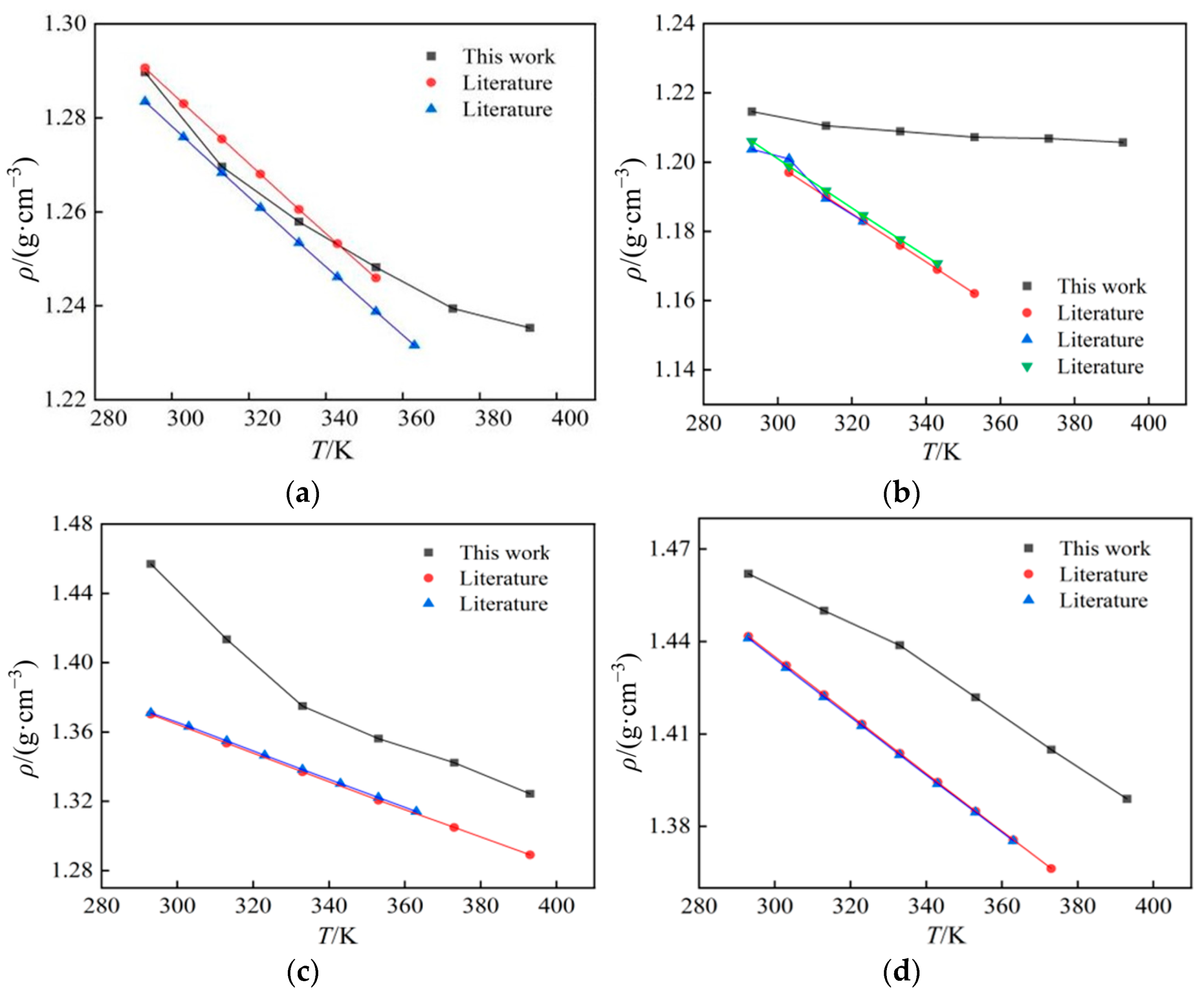
2.1. Density
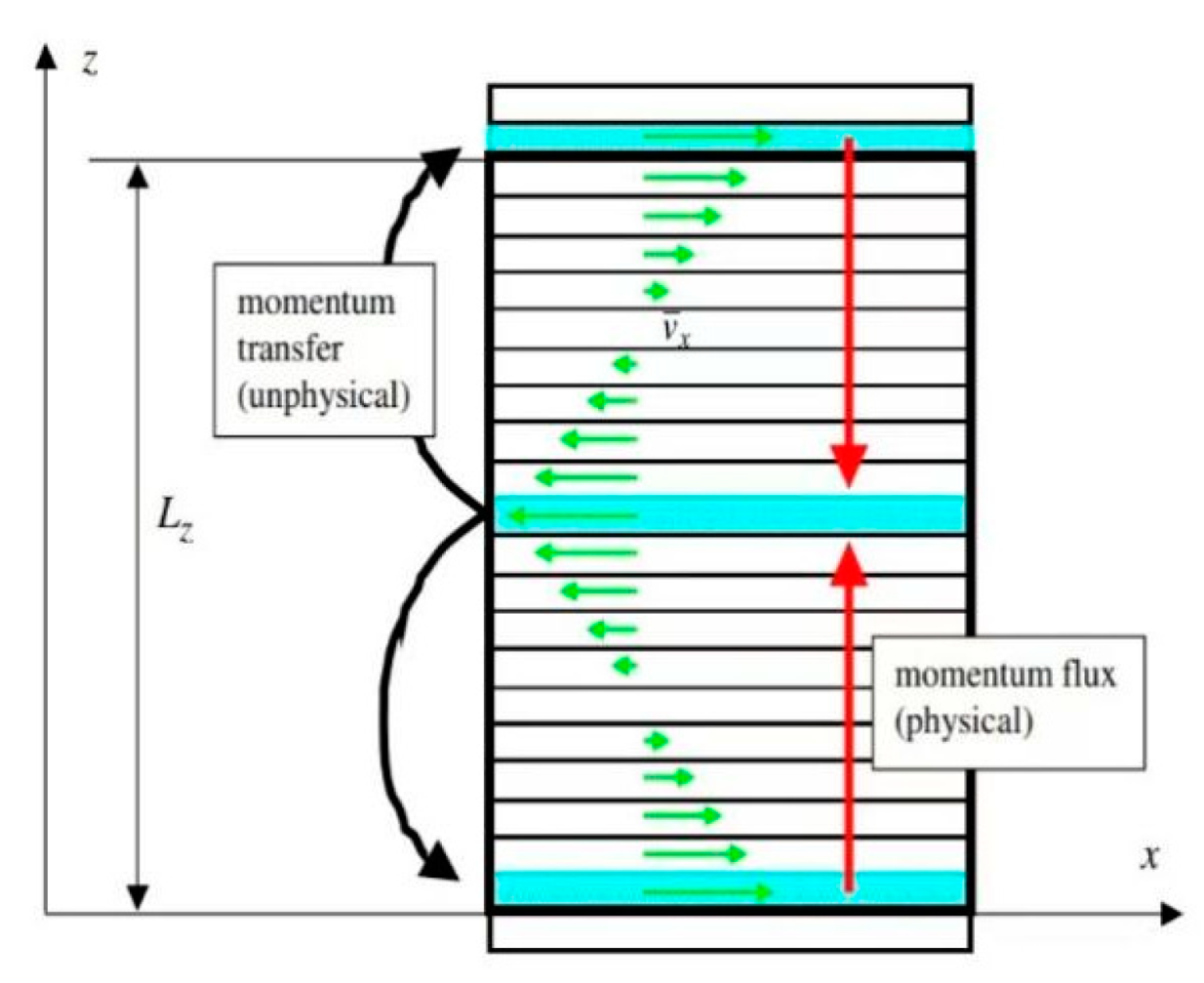
2.2. Viscosity
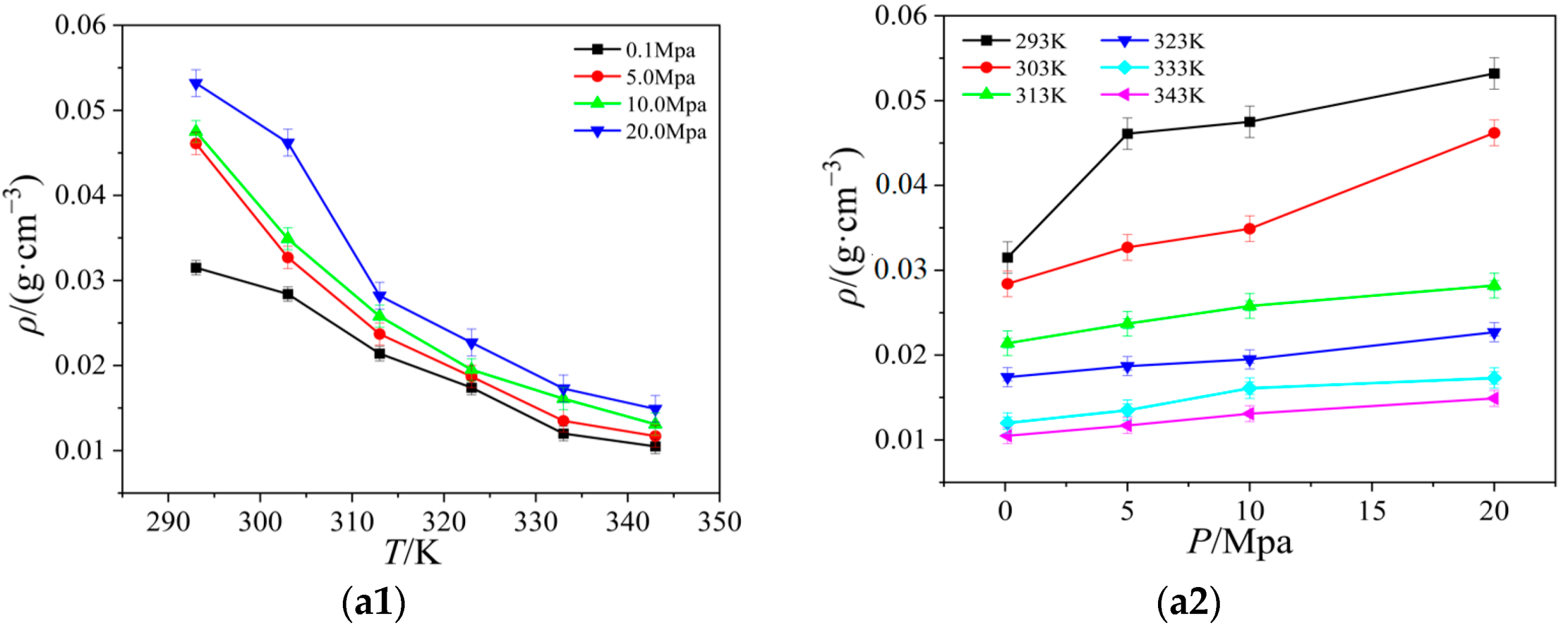
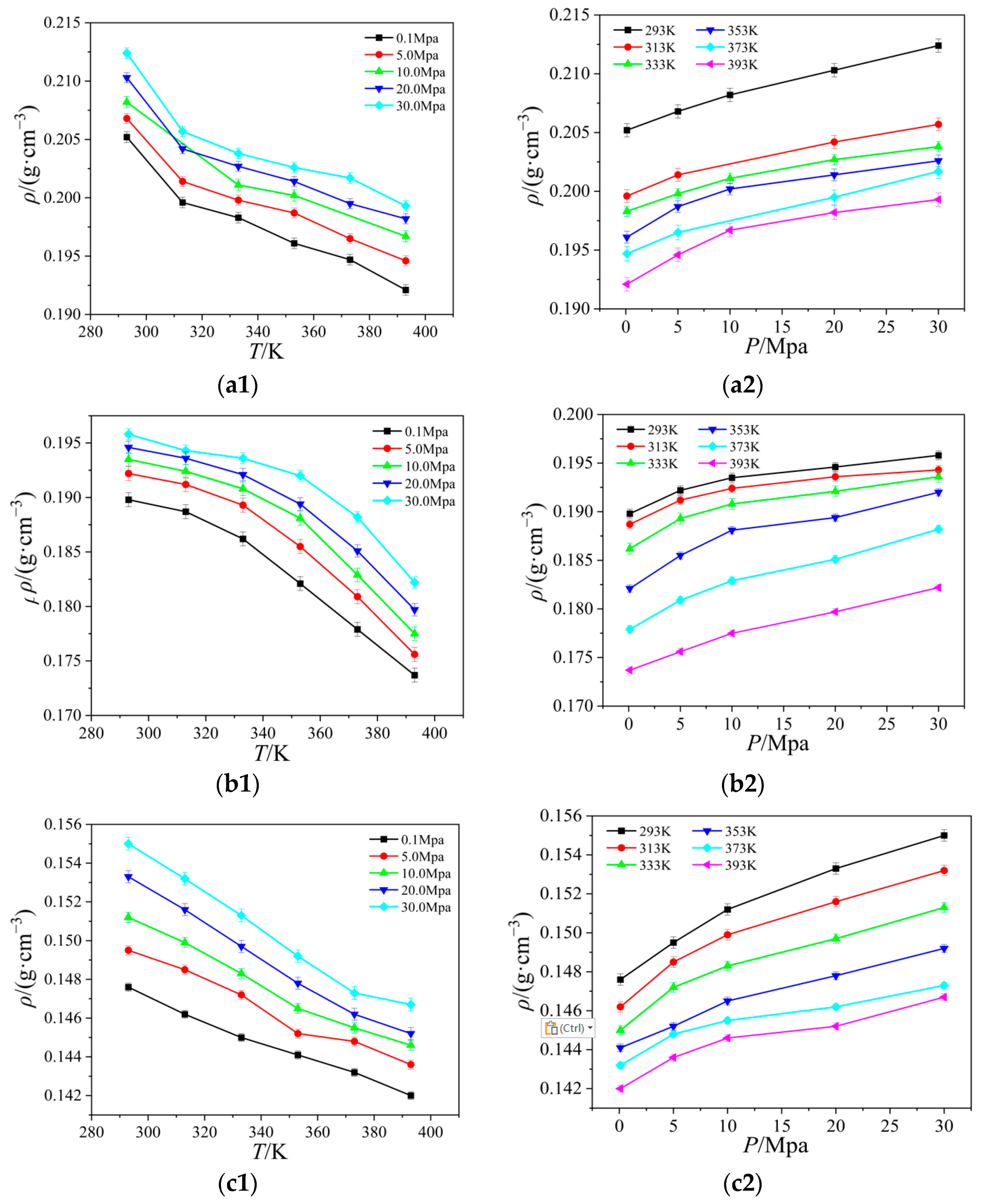
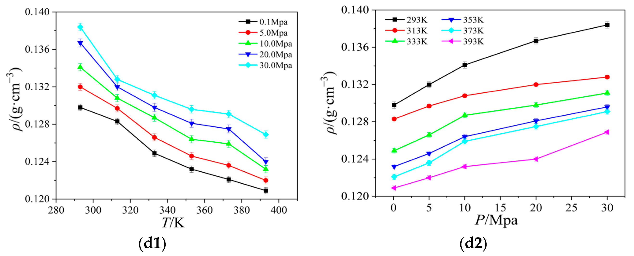
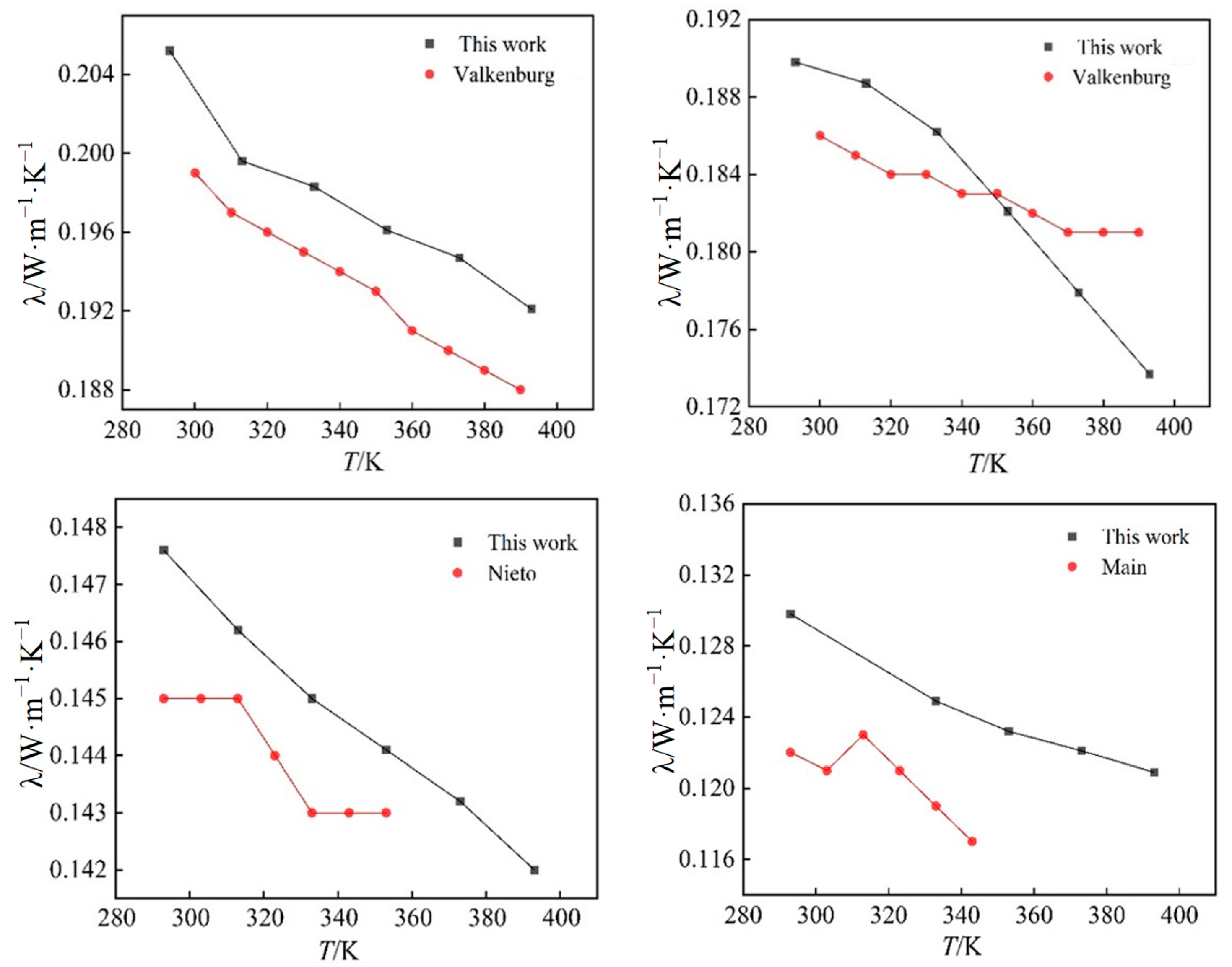
2.3. Thermal Conductivity
3. Materials and Methods
3.1. The Model of Calculating
3.2. Simulated Force Field
4. Conclusions
Author Contributions
Funding
Institutional Review Board Statement
Informed Consent Statement
Data Availability Statement
Conflicts of Interest
References
- Lingala, S.S. Ionic-Liquid-Based Nanofluids and Their Heat-Transfer Applications: A Comprehensive Review. ChemPhysChem 2023, 24, e202300191. [Google Scholar] [CrossRef] [PubMed]
- Minea, A.A. Overview of Ionic Liquids as Candidates for New Heat Transfer Fluids. Int. J. Thermophys. 2020, 41, 151. [Google Scholar] [CrossRef]
- Musiał, M.; Malarz, K.; Mrozek-Wilczkiewicz, A.; Musiol, R.; Zorębski, E.; Dzida, M. Pyrrolidinium-Based Ionic Liquids as Sustainable Media in Heat-Transfer Processes. ACS Sustain. Chem. Eng. 2017, 5, 11024–11033. [Google Scholar] [CrossRef]
- Liu, H.; Maginn, E.; Visser, A.E.; Bridges, N.J.; Fox, E.B. Thermal and Transport Properties of Six Ionic Liquids: An Lexperimental and Molecular Dynamics Study. Ind. Eng. Chem. Res. 2012, 51, 7242–7254. [Google Scholar] [CrossRef]
- Goloviznina, K.; Gong, Z.; Padua, A.A.H. The CL & Pol polarizable force field for the simulation of ionic liquids and eutectic solvents. Wiley Interdiscip. Rev. Comput. Mol. Sci. 2022, 12, e1572. [Google Scholar] [CrossRef]
- Bedrov, D.; Piquemal, J.-P.; Borodin, O.; MacKerell, A.D., Jr.; Roux, B.; Schröder, C. Molecular Dynamics Simulations of Ionic Liquids and Electrolytes Using Polarizable Force Fields. Chem. Rev. 2019, 119, 7940–7995. [Google Scholar] [CrossRef]
- Wang, T.; Liu, X.; He, M. Molecular dynamics simulations of ionic liquids [BMIM][Tf2N]. CIESC J. 2019, 70, 258–264. [Google Scholar] [CrossRef]
- Li, H.; Zhu, Y.; Chu, M.; Dong, H.; Zhang, G. Thermal conductivity of irregularly shaped nanoparticles from equilibrium molecular dynamics. J. Phys. Condens. Matter. 2024. [Google Scholar] [CrossRef]
- Soddemann, T.; Dünweg, B.; Kremer, K. Dissipative Particle Dynamics: A Useful Thermostat for Equilibrium and Nonequilibrium Molecular Dynamics Simulations. Phys. Rev. E 2003, 68, 046702. [Google Scholar] [CrossRef]
- Liu, Y.; Bian, Y.; Aleksandr, C.; Han, Z. Effect of Grain Boundary Angle on the Thermal Conductivity of Nanostructured Bicrystal ZnO Based on the Molecular Dynamics Simulation Method. Int. J. Heat Mass Tran. 2019, 145, 118791. [Google Scholar] [CrossRef]
- Norouzi, S.; Fakhrabadi, M.M.S. Anisotropic Nature of Thermal Conductivity in Graphene Spirals Revealed by Molecular Dynamics Simulations. J. Phys. Chem. Solid. 2019, 137, 109228. [Google Scholar] [CrossRef]
- Deng, X.; Wu, Z.; Wang, G. Thermal Conductivity and Heat Capacity of Water/Iβ Cellulose Nanofluids: A Molecular Dynamics Study. Int. J. Mod. Phys. B 2020, 34, 2050248. [Google Scholar] [CrossRef]
- Müller, T.J.; Müller-Plathe, F. Determining the Local Shear Viscosity of a Lipid Bilayer System by Reverse Non-Equilibrium Molecular Dynamics Simulations. Chemphyschem A Eur. J. Chem. Phys. Phys. Chem. 2010, 10, 2305–2315. [Google Scholar] [CrossRef] [PubMed]
- Seifert, E. OriginPro 9.1: Scientific data analysis and graphing software-software review. J. Chem. Inf. Model. 2014, 54, 1552. [Google Scholar] [CrossRef] [PubMed]
- Ciocirlan, O.; Croitoru, O.; Iulian, O. Density and Refractive Index of Binary Mixtures of Two 1-Alkyl-3-Methylimidazolium Ionic Liquids with 1,4-Dioxane and Ethylene Glycol. J. Chem. Eng. Data 2014, 59, 1165–1174. [Google Scholar] [CrossRef]
- Watanabe, M.; Kodama, D.; Makino, T.; Kanakubo, M. CO2 Absorption Properties of Imidazolium Based Ionic Liquids Using a Magnetic Suspension Balance. Fluid Phase Equilibria 2016, 420, 44–49. [Google Scholar] [CrossRef]
- Iwasaki, K.; Yoshii, K.; Tsuda, T.; Kuwabata, S. Physicochemical properties of Phenyltrifluoroborate-based Room Temperature Ionic Liquids. J. Mol. Liq. 2017, 246, 236–243. [Google Scholar] [CrossRef]
- Master, Z.; Malek, N.I. Temperature, Composition, and Alkyl Chain-Dependent Molecular Interactions Between Imidazolium-Based Ionic Liquids with N-Methylaniline and N-Ethylaniline: Experimental and Theoretical Study. J. Chem. Eng. Data ACS J. Data 2020, 65, 5249–5265. [Google Scholar] [CrossRef]
- Ebrahiminejadhasanabadi, M.; Nelson, W.M.; Naidoo, P.; Mohammadi, A.H.; Ramjugernath, D. Experimental Measurement of Carbon Dioxide Solubility in 1-Methylpyrrolidin-2-one (NMP)+1-Butyl-3-Methyl-1H-imidazol-3-ium Tetrafluoroborate ([Bmim][BF4]) Mixtures Using a New Static-Synthetic cell. Fluid Phase Equilibria 2018, 477, 62–77. [Google Scholar] [CrossRef]
- Safarov, J.; Suleymanli, K.; Aliyev, A.; Yeadon, D.J.; Jacquemin, J.; Bashirov, M.; Hassel, E. (p,rho,T) Data of 1-butyl-3-Methylimi-dazolium Hexafluorophosphate. J. Chem. Thermodyn. 2020, 141, 105954. [Google Scholar] [CrossRef]
- Koller, T.M.; Lenahan, F.D.; Schmidt, P.S.; Klein, T.; Mehler, J.; Maier, F.; Rausch, M.H.; Wasserscheid, P.; Steinrück, H.-P.; Fröba, A.P. Surface Tension and Viscosity of Binary Mixtures of the Fluorinated and Non-Fluorinated Ionic Liquids [BMIM][PF6] and [C(4)C(1)Im][PF6] by the Pendant Drop Method and Surface Light Scattering. Int. J. Thermophys. 2020, 41, 144. [Google Scholar] [CrossRef]
- Martins, M.A.R.; Sharma, G.; Pinho, S.P.; Gardas, R.L.; Coutinho, J.A.P.; Carvalho, P.J. Selection and Characterization of Non-ideal Ionic Liquids Mixtures to be Used in CO2 Capture. Fluid Phase Equilibria. 2020, 518, 112621. [Google Scholar] [CrossRef]
- Almeida, H.F.D.; Lopes, J.N.C.; Rebelo, L.P.N.; Coutinho, J.A.P.; Freire, M.G.; Marrucho, I.M. Densities and Viscosities of Mixtures of Two Ionic Liquids Containing a Common Cation. J. Chem. Eng. Data 2016, 61, 2828–2843. [Google Scholar] [CrossRef]
- Pameté, E.; Gorska, B.; Beguin, F. Mixtures of Ionic Liquids Based on EMIM Cation and Fluorinated Anions: Physico-Chemical Characterization in View of Their Application as Low-Temperature Electrolytes. J. Mol. Liq. 2020, 298, 111959. [Google Scholar] [CrossRef]
- Yang, X.; Fang, Y. A Volumetric and Viscosity Study for the Binary Mixtures of Ammonium-Based Asymmetrical Gemini Ionic Liquids with Alcohols at T=293.15-333.15K. J. Chem. Eng. Data 2019, 64, 722–735. [Google Scholar] [CrossRef]
- Bouarab, A.F.; Martins, M.A.R.; Stolarska, O.; Smiglak, M.; Harvey, J.-P.; Coutinho, J.A.P.; Robelin, C. Physical Properties and Solid-liquid Equilibria for Hexafluorophosphate-based Ionic Liquid Ternary Mixtures and Their Corresponding Subsystems. J. Mol. Liq. 2020, 316, 113742. [Google Scholar] [CrossRef]
- Thompson, A.P.; Aktulga, H.M.; Berger, R.; Bolintineanu, D.S.; Brown, W.M.; Crozier, P.S.; in’t Veld, P.J.; Kohlmeyer, A.; Moore, S.G.; Nguyen, T.D.; et al. LAMMPS-a flexible simulation tool for particle-based materials modeling at the atomic, meso, and continuum scales. Comput. Phys. Commun. 2022, 271, 108171. [Google Scholar] [CrossRef]
- Kundu, P.K.; Cohen, I.M.; Dowling, D.R. Fluid Mechanics; Academic Press: Cambridge, MA, USA, 2015. [Google Scholar] [CrossRef]
- Fourier, J.B.J. Théorie Analytique de la Chaleur; Gauthier-Villars, Imprimeur-Libraire: Paris, France, 1888. [Google Scholar] [CrossRef]
- Sambasivarao, S.V.; Acevedo, O. Development of OPLS-AA Force Field Parameters for 68 Unique Ionic Liquids. J. Chem. Theory Comput. 2009, 5, 1038–1050. [Google Scholar] [CrossRef]
- Watanabe, M.; Thomas, M.L.; Zhang, S.; Ueno, K.; Yasuda, T.; Dokko, K. Application of Ionic Liquids to Energy Storage and Conversion Materials and Devices. Chem. Rev. 2017, 117, 7190–7239. [Google Scholar] [CrossRef]
- Levesque, D.; Verlet, L.; Krkijarvi, J. Computer “’Experiments”’ on Classical Fluids. IV. Transport Properties and Time-Correlation Functions of the Lennard-Jones Liquid near its triple point. Phys. Rev. 1973, 7, 1690–1700. [Google Scholar] [CrossRef]
- Nicolas, J.J.; Gubbins, K.E.; Streett, W.B.; Tildesley, D.J. Equation of state for the Lennard-Jones fluid. Mol. Phys. 1979, 37, 1429–1454. [Google Scholar] [CrossRef]
- Johnson, J.K.; Mueller, E.A.; Gubbins, K.E. Equation of state for Lennard-Jones chains. J. Phys. Chem. 1994, 98, 6413–6419. [Google Scholar] [CrossRef]


| Ionic Liquids | [Emim][BF4] | [Bmim][BF4] | [Bmim][PF6] | [Bmim][Tf2N] |
|---|---|---|---|---|
| ηcal/pa·s | 0.0315 | 0.1323 | 0.3498 | 0.0604 |
| ηlit/pa·s | 0.0346 [24] | 0.1360 [25] | 0.3740 [26] | 0.0651 [24] |
| Dev.% | −8.96% | −2.72% | −6.47% | −7.39% |
| Atomic Type | q (e−) | ε (Kcal/mol) | σ (Å) |
|---|---|---|---|
| BF4 | |||
| B | 0.8276 | 0.095 | 3.5814 |
| F | −0.4569 | 0.060 | 3.1181 |
| PF6 | |||
| P | 1.3400 | 0.2000 | 3.7400 |
| F | −0.3900 | 0.0061 | 3.1181 |
| NTF2 | |||
| F | −0.1600 | 0.0530 | 2.9500 |
| C | 0.3500 | 0.0660 | 3.5000 |
| S | 1.0200 | 0.2500 | 3.5500 |
| O | −0.5300 | 0.2100 | 2.9600 |
| N | −0.6600 | 0.1700 | 3.2500 |
| EMIM | |||
| CR | −0.09 | 0.07 | 3.55 |
| CW | −0.24 | 0.07 | 3.55 |
| CW | −0.24 | 0.07 | 3.55 |
| HR | 0.21 | 0.03 | 2.42 |
| HW | 0.27 | 0.03 | 2.42 |
| HW | 0.27 | 0.03 | 2.42 |
| CM | −0.35 | 0.066 | 3.55 |
| HM | 0.18 | 0.03 | 2.55 |
| HM | 0.18 | 0.03 | 2.55 |
| HM | 0.18 | 0.03 | 2.55 |
| NA | 0.22 | 0.17 | 3.25 |
| CA | −0.17 | 0.066 | 3.5 |
| HA | 0.18 | 0.03 | 2.5 |
| CT | −0.24 | 0.066 | 3.5 |
| HT | 0.08 | 0.03 | 2.5 |
| HT | 0.08 | 0.03 | 2.5 |
| HT | 0.08 | 0.03 | 2.5 |
| NA | 0.22 | 0.17 | 3.25 |
| HA | 0.18 | 0.03 | 2.5 |
| BMIM | |||
| NA | 0.22 | 0.17 | 3.25 |
| NA | 0.22 | 0.17 | 3.25 |
| CR | −0.09 | 0.07 | 3.55 |
| HR | 0.21 | 0.03 | 2.42 |
| CW | −0.24 | 0.07 | 3.55 |
| HW | 0.27 | 0.03 | 2.42 |
| CW | −0.24 | 0.07 | 3.55 |
| HW | 0.27 | 0.03 | 2.42 |
| CM | −0.35 | 0.066 | 3.5 |
| HM | 0.18 | 0.03 | 2.42 |
| HM | 0.18 | 0.03 | 2.42 |
| HM | 0.18 | 0.03 | 2.42 |
| CA | −0.17 | 0.066 | 3.5 |
| HA | 0.18 | 0.03 | 2.42 |
| HA | 0.18 | 0.03 | 2.42 |
| CS | −0.12 | 0.066 | 3.5 |
| HS | 0.06 | 0.03 | 2.42 |
| HS | 0.06 | 0.03 | 2.42 |
| CS | −0.12 | 0.066 | 3.5 |
| HS | 0.06 | 0.03 | 2.42 |
| HS | 0.06 | 0.03 | 2.42 |
| CT | −0.24 | 0.066 | 3.5 |
| HT | 0.08 | 0.03 | 2.42 |
| HT | 0.08 | 0.03 | 2.42 |
Disclaimer/Publisher’s Note: The statements, opinions and data contained in all publications are solely those of the individual author(s) and contributor(s) and not of MDPI and/or the editor(s). MDPI and/or the editor(s) disclaim responsibility for any injury to people or property resulting from any ideas, methods, instructions or products referred to in the content. |
© 2024 by the authors. Licensee MDPI, Basel, Switzerland. This article is an open access article distributed under the terms and conditions of the Creative Commons Attribution (CC BY) license (https://creativecommons.org/licenses/by/4.0/).
Share and Cite
Fan, J.; Pan, Y.; Gao, Z.; Qu, H. Molecular Dynamic Simulations of the Physical Properties of Four Ionic Liquids. Int. J. Mol. Sci. 2024, 25, 11217. https://doi.org/10.3390/ijms252011217
Fan J, Pan Y, Gao Z, Qu H. Molecular Dynamic Simulations of the Physical Properties of Four Ionic Liquids. International Journal of Molecular Sciences. 2024; 25(20):11217. https://doi.org/10.3390/ijms252011217
Chicago/Turabian StyleFan, Jing, Yuting Pan, Zhiqiang Gao, and Hongwei Qu. 2024. "Molecular Dynamic Simulations of the Physical Properties of Four Ionic Liquids" International Journal of Molecular Sciences 25, no. 20: 11217. https://doi.org/10.3390/ijms252011217
APA StyleFan, J., Pan, Y., Gao, Z., & Qu, H. (2024). Molecular Dynamic Simulations of the Physical Properties of Four Ionic Liquids. International Journal of Molecular Sciences, 25(20), 11217. https://doi.org/10.3390/ijms252011217