
Combined FCS and PCH Analysis to Quantify Protein Dimerization in Living Cells

 , ,
, , 
 and
and
Abstract
:1. Introduction
2. Results and Discussion
2.1. Optimization of the BDGA Method in Order to Measure Monomer-Dimer Equilibria
2.1.1. Initial Steps in the Analysis of FFS Data
2.1.2. Two-Component BDGA of Lysate Mixtures
2.1.3. One-Component BDGA of Lysate Mixes
2.2. Improved BDGA Methodology for the Analysis of Cellular Data
2.3. Application of the Developed Methodology to the Analysis of Induced Dimerization in Cells
3. Materials and Methods
3.1. Theory of the Global Analysis of ACF and PCD
- Calculate the time dependent parametersfor each molecular species i = 1, 2, …, where T is the counting time interval (bin time), B2(T) is the binning correction factorcalculated over a time dependent term of the autocorrelation function in FCSand q0eff i, N0eff i, a, Ftrip, τtrip, τdiff i are fit parameters;
- Calculate single-molecular PCD for each molecular species iwhere k = 1, 2, …, K is the number of photons detected in an interval T, K is the maximal number of photons, Fcn, n = 1, 2 are instrumental out-of-focus correction parameters (Fcn are also fit parameters) andIn Equation (6), γ() is the incomplete gamma function and parameter Θ is varied depending on the value of the product of qeff T (from 1 to 20), see details in [38];
- Calculate PCD P(k) for each brightness component assuming the Poissonian distribution of a number of molecules in an open observation volumewhere is M-times convolution of the single-molecule PCD and Poi(k,η) denotes the Poisson distribution with the mean value η;
- Calculate the total PCD for a molecular system. PCD of a number of independent species is given by a convolution of PCD of each species
- The correction on dead-time is performed accordingly to the following equation [39]:where τdt is the detector dead time (fit parameter) and Pbinomial(j, n, p) is the binomial probability distribution. We omitted the dependence on T from qeff i, Neff i, and therefore from all related expressions in the Equations (5)–(9) for the sake of simplicity.
3.2. Sample Preparation and Measurement
3.2.1. Plasmids and Cloning
3.2.2. Cell Culture
3.2.3. Measurement in Cell Lysate
3.2.4. Measurement of Cells
3.3. Data Analysis Procedure
3.3.1. Fitting Software
3.3.2. Analysis of the Obtained Data
4. Conclusions
Supplementary Materials
Author Contributions
Funding
Institutional Review Board Statement
Informed Consent Statement
Conflicts of Interest
References
- Khokhlatchev, A.V.; Canagarajah, B.; Wilsbacher, J.; Robinson, M.; Atkinson, M.; Goldsmith, E.; Cobb, M.H. Phosphorylation of the MAP kinase ERK2 promotes its homodimerization and nuclear translocation. Cell 1998, 93, 605–615. [Google Scholar] [CrossRef] [Green Version]
- Brummer, T.; McInnes, C. RAF kinase dimerization: Implications for drug discovery and clinical outcomes. Oncogene 2020, 39, 4155–4169. [Google Scholar] [CrossRef] [PubMed]
- Rajakulendran, T.; Sahmi, M.; Lefrançois, M.; Sicheri, F.; Therrien, M. A dimerization-dependent mechanism drives RAF catalytic activation. Nature 2009, 461, 542–545. [Google Scholar] [CrossRef] [PubMed]
- Yaşar, P.; Ayaz, G.; User, S.D.; Güpür, G.; Muyan, M. Molecular mechanism of estrogen–estrogen receptor signaling. Reprod. Med. Biol. 2017, 16, 4–20. [Google Scholar] [CrossRef] [PubMed]
- Levin, E.R.; Hammes, S.R. Nuclear receptors outside the nucleus: Extranuclear signalling by steroid receptors. Nat. Rev. Mol. Cell Biol. 2016, 17, 783–797. [Google Scholar] [CrossRef] [PubMed] [Green Version]
- Shizu, R.; Yokobori, K.; Perera, L.; Pedersen, L.; Negishi, M. Ligand induced dissociation of the AR homodimer precedes AR monomer translocation to the nucleus. Sci. Rep. 2019, 9. [Google Scholar] [CrossRef] [PubMed]
- Jiménez-Panizo, A.; Pérez, P.; Rojas, A.M.; Fuentes-Prior, P.; Estébanez-Perpiñá, E. Non-canonical dimerization of the androgen receptor and other nuclear receptors: Implications for human disease. Endocr. Relat. Cancer 2019, 26, R479–R497. [Google Scholar] [CrossRef] [PubMed] [Green Version]
- Mahajan, N.P.; Linder, K.; Berry, G.; Gordon, G.W.; Heim, R.; Herman, B. Bcl-2 and bax interactions in mitochondria probed with green fluorescent protein and fluorescence resonance energy transfer. Nat. Biotechnol. 1998, 16, 547–552. [Google Scholar] [CrossRef] [PubMed]
- Bacia, K.; Kim, S.A.; Schwille, P. Fluorescence cross-correlation spectroscopy in living cells. Nat. Methods 2006, 3, 83–89. [Google Scholar] [CrossRef]
- Jameson, D.M.; Ross, J.A.; Albanesi, J.P. Fluorescence fluctuation spectroscopy: Ushering in a new age of enlightenment for cellular dynamics. Biophys. Rev. 2009, 1, 105–118. [Google Scholar] [CrossRef]
- Kitamura, A.; Kinjo, M. State-of-the-art fluorescence fluctuation-based spectroscopic techniques for the study of protein aggregation. Int. J. Mol. Sci. 2018, 19, 964. [Google Scholar] [CrossRef] [Green Version]
- Wu, B.; Singer, R.H.; Mueller, J.D. Time-integrated fluorescence cumulant analysis and its application in living cells. In Methods in Enzymology; Academic Press Inc.: Cambridge, MA, USA, 2013; Volume 518, pp. 99–119. ISBN 9780123884220. [Google Scholar]
- Nagy, P.; Claus, J.; Jovin, T.M.; Arndt-Jovin, D.J. Distribution of resting and ligand-bound ErbB1 and ErbB2 receptor tyrosine kinases in living cells using number and brightness analysis. Proc. Natl. Acad. Sci. USA 2010, 107, 16524–16529. [Google Scholar] [CrossRef] [Green Version]
- Sarkar-Banerjee, S.; Sayyed-Ahmad, A.; Prakash, P.; Cho, K.J.; Waxham, M.N.; Hancock, J.F.; Gorfe, A.A. Spatiotemporal Analysis of K-Ras Plasma Membrane Interactions Reveals Multiple High Order Homo-oligomeric Complexes. J. Am. Chem. Soc. 2017, 139, 13466–13475. [Google Scholar] [CrossRef]
- Chen, Y.; Wei, L.-N.; Müller, J.D. Probing protein oligomerization in living cells with fluorescence fluctuation spectroscopy. Proc. Natl. Acad. Sci. USA 2003, 100, 15492–15497. [Google Scholar] [CrossRef] [Green Version]
- Saffarian, S.; Li, Y.; Elson, E.L.; Pikey, L.J. Oligomerization of the EGF receptor investigated by live cell fluorescence intensity distribution analysis. Biophys. J. 2007, 93, 1021–1031. [Google Scholar] [CrossRef] [PubMed] [Green Version]
- Kask, P.; Palo, K.; Ullmann, D.; Gall, K. Fluorescence-intensity distribution analysis and its application in biomolecular detection technology. Proc. Natl. Acad. Sci. USA 1999, 96, 13756–13761. [Google Scholar] [CrossRef] [Green Version]
- Palo, K.; Mets, Ü.; Jäger, S.; Kask, P.; Gall, K. Fluorescence intensity multiple distributions analysis: Concurrent determination of diffusion times and molecular brightness. Biophys. J. 2000, 79, 2858–2866. [Google Scholar] [CrossRef] [Green Version]
- Politz, J.C.; Browne, E.S.; Wolf, D.E.; Pederson, T. Intranuclear diffusion and hybridization state of oligonucleotides measured by fluorescence correlation spectroscopy in living cells. Proc. Natl. Acad. Sci. USA 1998, 95, 6043–6048. [Google Scholar] [CrossRef] [PubMed] [Green Version]
- Schwille, P.; Haupts, U.; Maiti, S.; Webb, W.W. Molecular dynamics in living cells observed by fluorescence correlation spectroscopy with one- and two-photon excitation. Biophys. J. 1999, 77, 2251–2265. [Google Scholar] [CrossRef] [Green Version]
- Pan, P.-Y.; Li, X.; Wang, J.; Powell, J.; Wang, Q.; Zhang, Y.; Chen, Z.; Wicinski, B.; Hof, P.; Ryan, T.A.; et al. Parkinson’s Disease-Associated LRRK2 Hyperactive Kinase Mutant Disrupts Synaptic Vesicle Trafficking in Ventral Midbrain Neurons. J. Neurosci. 2017, 37, 11366–11376. [Google Scholar] [CrossRef] [PubMed]
- Chen, Y.; Müller, J.D.; So, P.T.C.; Gratton, E. The photon counting histogram in fluorescence fluctuation spectroscopy. Biophys. J. 1999, 77, 553–567. [Google Scholar] [CrossRef] [Green Version]
- Muller, J.D.; Chen, Y.; Gratton, E. Resolving heterogeneity on the single molecular level with the photon-counting histogram. Biophys. J. 2000, 78, 474–486. [Google Scholar] [CrossRef] [Green Version]
- Werner, A.; Skakun, V.V.; Meyer, C.; Hahn, U. RNA dimerization monitored by fluorescence correlation spectroscopy. Eur. Biophys. J. 2011, 40, 907–921. [Google Scholar] [CrossRef]
- Oasa, S.; Sasaki, A.; Yamamoto, J.; Mikuni, S.; Kinjo, M. Homodimerization of glucocorticoid receptor from single cells investigated using fluorescence correlation spectroscopy and microwells. FEBS Lett. 2015, 589, 2171–2178. [Google Scholar] [CrossRef] [Green Version]
- Skakun, V.V.; Engel, R.; Digris, A.V.; Borst, J.W.; Visser, A.J.W.G. Global analysis of autocorrelation functions and photon counting distributions. Front. Biosci. Elit. 2011, 3, 489–505. [Google Scholar] [CrossRef] [PubMed] [Green Version]
- Skakun, V.V.; Engel, R.; Borst, J.W.; Apanasovich, V.V.; Visser, A.J.W.G. Simultaneous diffusion and brightness measurements and brightness profile visualization from single fluorescence fluctuation traces of GFP in living cells. Eur. Biophys. J. 2012, 41, 1055–1064. [Google Scholar] [CrossRef]
- Spencer, D.M.; Wandless, T.J.; Schreiber, S.L.; Crabtree, G.R. Controlling signal transduction with synthetic ligands. Science 1993, 262, 1019–1024. [Google Scholar] [CrossRef]
- Guan, Y.; Meurer, M.; Raghavan, S.; Rebane, A.; Lindquist, J.R.; Santos, S.; Kats, I.; Davidson, M.W.; Mazitschek, R.; Hughes, T.E.; et al. Live-cell multiphoton fluorescence correlation spectroscopy with an improved large Stokes shift fluorescent protein. Mol. Biol. Cell 2015, 26, 2054–2066. [Google Scholar] [CrossRef] [PubMed]
- Skakun, V.V.; Hink, M.A.; Digris, A.V.; Engel, R.; Novikov, E.G.; Apanasovich, V.V.; Visser, A.J.W.G. Global analysis of fluorescence fluctuation data. Eur. Biophys. J. 2005, 34, 323–334. [Google Scholar] [CrossRef]
- Davis, L.; Shen, G. Accounting for Triplet and Saturation Effects in FCS Measurements. Curr. Pharm. Biotechnol. 2006, 7, 287–301. [Google Scholar] [CrossRef] [Green Version]
- Widengren, J.; Mets, Ü.; Rigler, R. Fluorescence correlation spectroscopy of triplet states in solution: A theoretical and experimental study. J. Phys. Chem. 1995, 99, 13368–13379. [Google Scholar] [CrossRef]
- Vámosi, G.; Mücke, N.; Müller, G.; Krieger, J.W.; Curth, U.; Langowski, J.; Tóth, K. EGFP oligomers as natural fluorescence and hydrodynamic standards. Sci. Rep. 2016, 6, 33022. [Google Scholar] [CrossRef] [PubMed] [Green Version]
- Youker, R.T.; Teng, H. Measuring protein dynamics in live cells: Protocols and practical considerations for fluorescence fluctuation microscopy. J. Biomed. Opt. 2014, 19, 090801. [Google Scholar] [CrossRef] [PubMed] [Green Version]
- Dickson, R.M.; Cubittt, A.B.; Tsient, R.Y.; Moerner, W.E. On/off blinking and switching behaviour of single molecules of green fluorescent protein. Nature 1997, 388, 355–358. [Google Scholar] [CrossRef]
- Pruschy, M.N.; Spencer, D.M.; Kapoor, T.M.; Miyake, H.; Crabtree, G.R.; Schreiber, S.L. Mechanistic studies of a signaling pathway activated by the organic dimerizer FK1012. Chem. Biol. 1994, 1, 163–172. [Google Scholar] [CrossRef]
- Marquardt, D.W. An Algorithm for Least-Squares Estimation of Nonlinear Parameters. J. Soc. Ind. Appl. Math. 1963, 11, 431–441. [Google Scholar] [CrossRef]
- Skakun, V.V.; Digris, A.V.; Apanasovich, V.V. Global analysis of autocorrelation functions and photon counting distributions in fluorescence fluctuation spectroscopy. Methods Mol. Biol. 2014, 1076, 719–741. [Google Scholar] [CrossRef]
- Palo, K.; Mets, Ü.; Loorits, V.; Kask, P. Calculation of photon-count number distributions via master equations. Biophys. J. 2006, 90, 2179–2191. [Google Scholar] [CrossRef] [Green Version]
- Veltman, D.M.; Keizer-Gunnink, I.; Haastert, P.J.M.V. An extrachromosomal, inducible expression system for Dictyostelium discoideum. Plasmid 2009, 61, 119–125. [Google Scholar] [CrossRef] [Green Version]
- Kollmar, M. Use of the myosin motor domain as large-affinity tag for the expression and purification of proteins in Dictyostelium discoideum. Int. J. Biol. Macromol. 2006, 39, 37–44. [Google Scholar] [CrossRef]
- Bevington, P.R.; Robinson, D.K. Data Reduction and Error Analysis for the Physical Sciences, 3rd ed.; McGraw-Hill Publishing Company: New York City, NY, USA, 2003; ISBN 0072472278/9780072472271. [Google Scholar]
- Skakun, V.V.; Novikov, E.G.; Apanasovich, T.V.; Apanasovich, V.V. Fluorescence cumulants analysis with non-ideal observation Profiles. Methods Appl. Fluoresc. 2015, 3. [Google Scholar] [CrossRef] [PubMed]
- Matthews, J.M.; Sunde, M. Dimers, oligomers, everywhere. Adv. Exp. Med. Biol. 2012, 747, 1–18. [Google Scholar] [CrossRef] [PubMed]


| Sample | Analysis Method | Ftrip (×10−2) | τtrip (µs) | τdiff1 (µs) | N (±SD) | qtrue (×104 cpms) | SD of qtrue | χ2 |
|---|---|---|---|---|---|---|---|---|
| R110 | 1-component | 9.10 ± 0.78 | 6.9 ± 1.2 | 35 ± 1 | 4.50 (±0.06) | 4.04 ± 0.023 | 0.055 | 1.147 |
| GFP | 1-component | 12.2 ± 0.90 | 35.1 ± 2.0 | 151 ± 4 | 3.88 (±0.09) | 3.20 ± 0.020 | 0.096 | 1.05 |
| diGFP | 1-component | 7.08 ± 0.43 | 31.0 ± 2.0 | 221 ± 3 | 3.63 (±0.06) | 5.12 ± 0.023 | 0.090 | 1.233 |
| 50% GFP + 50% diGFP | 1-component | 8.97 ± 0.47 | 22.2 ± 2.5 | 191 ± 2 | 3.47 (±0.07) | 4.88 ± 0.025 | 0.107 | 1.193 |
| 2-component (r = 1.8) | 8.07 ± 0.46 | 19.1 ± 2.4 | 151 (τdiff1); 221 (τdiff2) | 2.00 (±0.18) (N1); 1.76 (±0.12) (N2) | 3.20 (q1); 5.76 (q2) | - | 1.068 |
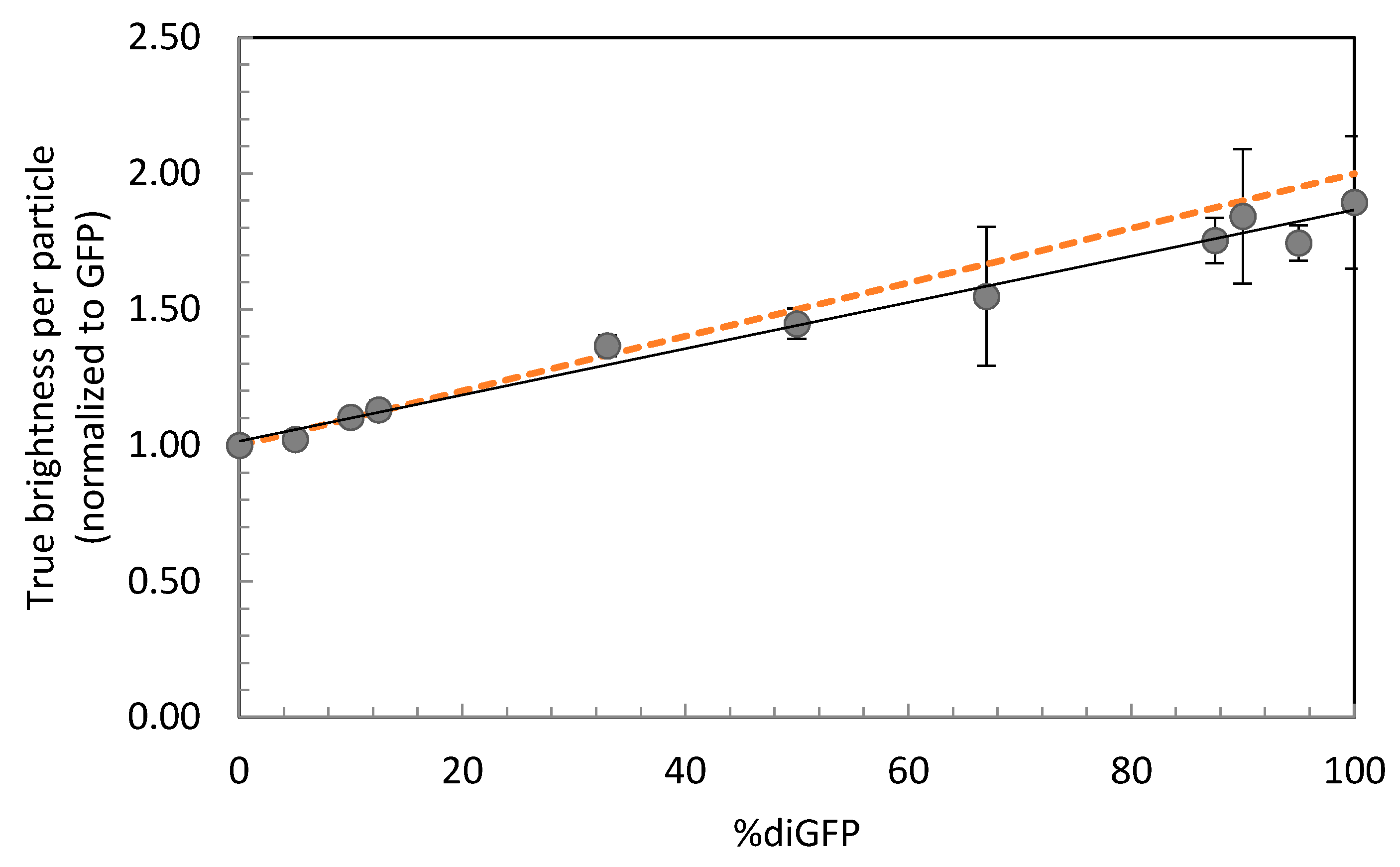
| diGFP% | τdiff (µs) | D (µm2 s−1) | qtrue (×104 cpms) | qtrue Norm. to GFP |
|---|---|---|---|---|
| 0 | 131 ± 21 | 97.3 ± 6.5 | 4.43 ± 1.22 | 1.00 ± 0.02 |
| 5 | 126 ± 32 | 98.3 ± 6.6 | 5.13 ± 1.19 | 1.02 ± 0.03 |
| 10 | 154 ± n.a. | 99.0 ± n.a. | 5.16 ± 1.60 | 1.10 ± 0.03 |
| 12.5 | 132 ± 37 | 94.1 ± 3.3 | 5.19 ± 1.15 | 1.13 ± 0.03 |
| 33.3 | 137 ± 32 | 87.7 ± 3.9 | 6.43 ± 1.42 | 1.37 ± 0.04 |
| 50 | 169 ± 31 | 74.0 ± 6.0 | 5.69 ± 1.62 | 1.45 ± 0.06 |
| 66.7 | 168 ± 37 | 78.4 ± 0.1 | 6.20 ± 1.84 | 1.55 ± 0.25 |
| 87.5 | 156 ± 37 | 76.8 ± 2.2 | 8.22 ± 2.02 | 1.75 ± 0.08 |
| 90 | 175 ± 46 | 69.5 ± 6.9 | 8.27 ± 2.88 | 1.84 ± 0.25 |
| 95 | 158 ± 36 | 75.7 ± 2.4 | 8.68 ± 1.70 | 1.74 ± 0.07 |
| 100 | 173 ± 40 | 71.4 ± 5.9 | 8.82 ± 2.77 | 1.89 ± 0.24 |
| Sample | Ftrip | τtrip (µs) | τdiff (µs) | N (range) | q (×104 cpms) | SD of q (×104 cpms) | # Traces | χ2 |
|---|---|---|---|---|---|---|---|---|
| GFP (trip free) | 0.241 ± 0.008 | 53.8 ± 2.8 | 381 ± 8 | 12.1 (8.5–19.9) | 4.71 ± 0.06 | 0.55 | 14 | 1.197 |
| GFP (trip fixed) | 0.178 | 40.0 | 330 ± 2 | 11 (7.8–18.2) | 5.18 ± 0.07 | 0.55 | 14 | 1.108 |
| diGFP | 0.128 | 61.9 | 841 ± 6 | 6.5 (4.9–7.9) | 8.32 ± 0.10 | 1.04 | 13 | 1.079 |
| FKBP12-GFP + dim | 0.178 | 40.0 | 1018 ± 9 | 19 (16.5–21.7) | 6.73 ± 0.18 | 0.79 | 9 | 1.015 |
| Sample | τdiff (µs) | D (µm2 s−1) | q (×104 cpms) | q Normalized to GFP | # Cells |
|---|---|---|---|---|---|
| GFP | 506 ± 115 | 16.7 ± 3.6 | 4.9 ± 0.6 | 1.00 ± 0.07 | 35 |
| diGFP | 871 ± 336 | 10.2 ± 2.4 * | 7.8 ± 1.4 | 1.60 ± 0.25 * | 27 |
| GFP + dim | 502 ± 133 | 17.1 ± 4.3 | 4.9 ± 0.6 | 1.00 ± 0.09 | 28 |
| FKBP12-GFP | 882 ± 269 | 9.8 ± 2.2 | 4.8 ± 0.7 | 0.98 ± 0.09 | 31 |
| FKBP12-GFP + dim | 1101 ± 336 | 7.8 ± 1.7 ** | 6.6 ± 0.9 | 1.33 ± 0.15 ** | 35 |
Publisher’s Note: MDPI stays neutral with regard to jurisdictional claims in published maps and institutional affiliations. |
© 2021 by the authors. Licensee MDPI, Basel, Switzerland. This article is an open access article distributed under the terms and conditions of the Creative Commons Attribution (CC BY) license (https://creativecommons.org/licenses/by/4.0/).
Share and Cite
Nederveen-Schippers, L.M.; Pathak, P.; Keizer-Gunnink, I.; Westphal, A.H.; van Haastert, P.J.M.; Borst, J.W.; Kortholt, A.; Skakun, V. Combined FCS and PCH Analysis to Quantify Protein Dimerization in Living Cells. Int. J. Mol. Sci. 2021, 22, 7300. https://doi.org/10.3390/ijms22147300
Nederveen-Schippers LM, Pathak P, Keizer-Gunnink I, Westphal AH, van Haastert PJM, Borst JW, Kortholt A, Skakun V. Combined FCS and PCH Analysis to Quantify Protein Dimerization in Living Cells. International Journal of Molecular Sciences. 2021; 22(14):7300. https://doi.org/10.3390/ijms22147300
Chicago/Turabian StyleNederveen-Schippers, Laura M., Pragya Pathak, Ineke Keizer-Gunnink, Adrie H. Westphal, Peter J. M. van Haastert, Jan Willem Borst, Arjan Kortholt, and Victor Skakun. 2021. "Combined FCS and PCH Analysis to Quantify Protein Dimerization in Living Cells" International Journal of Molecular Sciences 22, no. 14: 7300. https://doi.org/10.3390/ijms22147300
APA StyleNederveen-Schippers, L. M., Pathak, P., Keizer-Gunnink, I., Westphal, A. H., van Haastert, P. J. M., Borst, J. W., Kortholt, A., & Skakun, V. (2021). Combined FCS and PCH Analysis to Quantify Protein Dimerization in Living Cells. International Journal of Molecular Sciences, 22(14), 7300. https://doi.org/10.3390/ijms22147300