Abstract
The quantitative structure-activity relationship (QSAR) model searches for a reliable relationship between the chemical structure and biological activities in the field of drug design and discovery. (1) Background: In the study of QSAR, the chemical structures of compounds are encoded by a substantial number of descriptors. Some redundant, noisy and irrelevant descriptors result in a side-effect for the QSAR model. Meanwhile, too many descriptors can result in overfitting or low correlation between chemical structure and biological bioactivity. (2) Methods: We use novel log-sum regularization to select quite a few descriptors that are relevant to biological activities. In addition, a coordinate descent algorithm, which uses novel univariate log-sum thresholding for updating the estimated coefficients, has been developed for the QSAR model. (3) Results: Experimental results on artificial and four QSAR datasets demonstrate that our proposed log-sum method has good performance among state-of-the-art methods. (4) Conclusions: Our proposed multiple linear regression with log-sum penalty is an effective technique for both descriptor selection and prediction of biological activity.
1. Introduction
The quantitative structure-activity relationship (QSAR) model searches for a reliable relationship between chemical the structure and biological activities in the field of drug design and discovery [1]. In the study of QSAR, the chemical structure is encoded by a substantial number of descriptors, such as thermodynamic, shape descriptors, etc. Generally, only a few descriptors that are relevant to biological activities are of interest to the QSAR model. Descriptor selection aims to eliminate redundant, noisy and irrelevant descriptors [2]. The flow diagram shows the process of QSAR modeling in Figure 1.
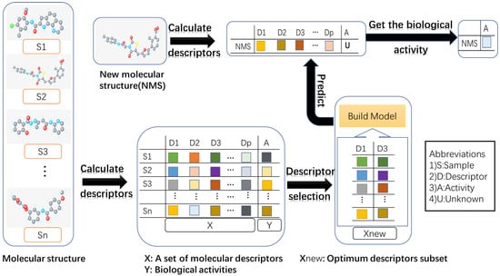
Figure 1.
The flow diagram shows the process of QSAR modeling. (1) Collecting molecular structures and their activities; (2) calculating molecular descriptors, which can produce thousands of parameters for each molecular structure; (3) removing redundant or irrelevant descriptors via descriptor selection; (4) building the model with the optimum descriptor subset; (5) predicting the biological activity of a new molecular structure using the established model. Different color blocks represent different values.
Generally, descriptor selection techniques can be categorized into four groups in the study of QSAR: classical methods, artificial intelligence-based methods, miscellaneous methods and regularization methods.
The classical methods have been proposed in the study of QSAR; as an example, forward selection adds the most significant descriptors until none improves the model to a statistically-significant extent. Backward elimination starts with all candidate descriptors, subsequently deleting descriptors without any statistical significance. Generally, stepwise regression builds a model by adding or removing predictor variables based on a series of F-tests or t-tests. The variable selection and modeling method based on the prediction [3] uses leave-one-out cross-validation (), predicted to select meaningful and important descriptors. Leaps-and-bounds regression [4] selects a subset of descriptors based on the residual sum of squares (RSS).
Recently, artificial intelligence-based methods have been designed for descriptor selection, such as the genetic algorithm [5], which uses the code, selection, exchange and mutation operations to select the important descriptors. Particle swarm optimization [6] has a series of initial random particles and then selects the descriptors by updating the velocity and positions. Artificial neural networks [7] are composed of many artificial neurons that are linked together according to a specific network architecture and select input nodes (descriptors) to predict the output node (biological activity). Simulated annealing [8] can be performed with the Metropolis algorithm based on Monte Carlo techniques, which performs descriptor selection. Frank et al. [9] used Bayesian regularized artificial neural networks with automatic relevance determination (ARD) in the study of QSAR. ARD has the capacity to allow the network to estimate the importance of each input, neglects irrelevant or highly correlated indices in the modeling and uses the most important variables for modeling the activity data. The ant colony system [10], inspired by real ants, searches a path, which is connected to a number of selected descriptors, between the colony and a source of food.
The miscellaneous methods used for descriptor selection in the development of QSAR include K nearest neighbor (KNN) [11], the replacement method (RM) [12], the successive projections algorithm (SPA) [13] and uninformative variable elimination-partial least squares (UVE-PLS) [14], just to name a few. KNN uses a similarity measure (Euler distance) to select the descriptor and predict the biological activity. RM has the capacity to find an optimal subset of the descriptors via the standard deviation. SPA is a simple operation to eliminate collinearity to reduce the descriptors. UVE-PLS has been proposed to increase the predictive ability of the standard PLS method via eliminating the variables that cannot contribute to the model and to make a comparison between experimental variables and added noise variables with respect to the degree of contribution to the model.
The regularization is an effective technique in descriptor selection and has been used in QSRR [15], QSPR [16] and QSTR [17] in the field of chemometrics. However, some individuals have poured their interest and attention into the study of QSAR. For example, LASSO () (least absolute shrinkage and selection operator) [18] has the capacity to perform descriptor selection. Algamal et al. proposed the -norm to select the significant and meaningful descriptors for anti-hepatitis C virus activity of thiourea derivatives in the QSAR classification model [19]. Xu et al. proposed [20] regularization, which has more sparsity. Algamal et al. proposed a penalized linear regression model with the -norm to select the significant and meaningful descriptors [21]. Theoretically, the regularization produces better solutions with more sparsity [22], but it is an NP problem. Therefore, Candes et al. proposed the log-sum penalty [23], which approximates the regularization much better.
In this paper, we utilized the log-sum penalty, which is non-convex in Figure 2. A coordinate descent algorithm, which uses novel univariate log-sum thresholding for updating the estimated coefficients, has been developed for the QSAR model. Experimental results on artificial and four QSAR datasets demonstrate that our proposed log-sum method has good performance among state-of-the-art methods. The structure of this paper is organized as follows: Section 2 introduces a coordinate descent algorithm, which uses novel univariate log-sum thresholding for updating the estimated coefficients and gives a detailed description of the datasets. In Section 3, we discuss the experimental results on simulated data and four QSRA datasets. Finally, we give some conclusions in Section 4.
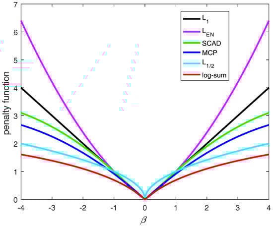
Figure 2.
and are convex, and SCAD, MCP, and log-sum are non-convex. The log-sum approximates to .
2. Methods
In this paper, there exists a predictor X and a response y, which represent the chemical structure and corresponding biological activities, respectively. Suppose we have n samples, , where = (, ,..., ) is the i-th input pattern with dimensionality p, which means has p descriptors, and denotes the value of descriptor j for the i-th sample. The multiple linear regression is expressed as:
where are the coefficients.
Given X and y, are estimated based on an objective function. The linear regression of the objective function can be formulated:
where is the vector of n response variables, X = {,,......,} is matrix with and denotes the -norm. When the number of variables is larger than the number of samples (), this can result in over-fitting. Here, we introduced a penalty function in the objective function to estimate the coefficient. We have rewritten Equation (2):
where is a penalty function indexed by the regularized parameter .
2.1. Coordinate Decent Algorithm for Different Thresholding Operators
In this paper, we used the coordinate descent algorithm to implement different penalized multiple linear regression. The algorithm is a “one-at-a-time” algorithm and solves , and other (representing the parameters remaining after the j-th element is removed) are fixed [22]. Equation (3) can be rewritten as:
where k represents other variables except the j-th variable.
Take the derivative with respect to :
Denote , , , where represents the partial residuals with respect to the j-th covariate. To take into account the correlation of descriptors, Zhou et al. have proposed elastic net () [24], which emphasizes a grouping effect. The penalty function is given as follows:
The penalty function of is a combination of the penalty () and the ridge penalty (). Therefore, Equation (5) is rewritten as follows:
Donoho et al. proposed the univariate solution [25] for a -penalized regression coefficient as follows:
where is the soft thresholding operator for the if a is equal to one; Formula (8) can be rewritten as follows:
Fan et al. have proposed the smoothly clipped absolute deviation (SCAD) [26], which can produce a sparse set of solutions and approximately unbiased coefficients for large coefficients. The penalty function is shown as follows:
Additionally, the SCAD thresholding operator is given as follows:
Similar to the SCAD penalty, Zhang et al. have proposed the maximum concave penalty (MCP) [27]. The formula of the penalty function is shown as:
Additionally, the MCP thresholding operator is given as follows:
where is the experience parameter.
Xu et al. proposed regularization [20]. Formula (3) can be rewritten:
and the univariate half thresholding operator for a -penalized linear regression coefficient is as follows:
where .
In this paper, we applied the log-sum penalty to the linear regression model. We could rewrite Formula (3) as follows:
where should be set arbitrarily small, to make the log-sum penalty closely resemble the -norm. Equation (16) has a local minimal. The proof is given in the Appendix A:
where and .
According to different thresholding operators, we can define three properties for to satisfy the coefficient estimator, unbiasedness, sparsity and continuity, in Figure 3.
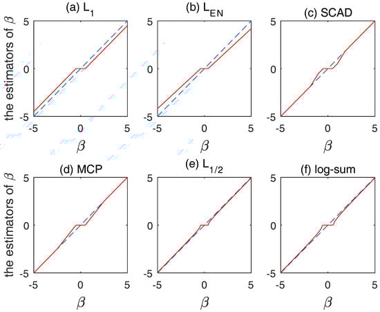
Figure 3.
Plot of thresholding functions for: (a) ; (b) ; (c) SCAD; (d) MCP; (e) ; and (f) log-sum.
2.2. Dataset
2.2.1. Simulated Data
In this work, we constructed the simulation. The process of the construction was given as follows:
Step I: The simulated dataset was generated from multiple linear regression using the normal distribution to produce X. Here, the number of row is sample n and the number of column is variable p.
where is the vector of n response variables, X = {, , ..., } is the generated matrix with , is the random error and controls the signal to noise.
Step II: Add a different correlation parameter to the simulation data.
Step III: In order to get a high quality model and variable selection, the coefficients (20) are set in advance from 1–20.
where is the coefficient.
In the simulation study, we firstly generated 100 groups of data with different sample sizes and . Secondly, the correlation coefficient and the noise control parameter , were considered in the model. Thirdly, the coefficients (20) are set in advance. Fourthly, the multiple linear regression with different penalties to select variables and build the model, including our proposed method, was used. Finally, due to the generation of 100 groups of data, the results obtained by different methods need to be averaged.
2.2.2. Real Data
We could obtain four public QSAR datasets, including the global half-life index [28], endocrine disruptor chemical (EDC) estrogen receptor (ER)-binding [29], (Benzo-)Triazoles toxicity in Daphnia magna [30] and apoptosis regulator Bcl-2 [31]. A brief description of these datasets is shown in Table 1. We utilized random sampling to divide datasets into training datasets and test datasets (80% for the training set and 20% for the test set [32]). Six commonly-used parameters in regression problems are employed to evaluate the model performance, including the square correlation coefficients of the leave-one-out cross-validation (), the root mean squared error of cross-validation (), the square correlation coefficients of fitting for the training set (), the root mean squared error for the training set (), the square correlation coefficients of fitting for the test set () and the root mean squared error for the test set (). According to existing literature [33], we have learned that the value of is not the best measure for QSAR model evaluation. Therefore, we poured more interest and attention into () and ().
| Algorithm: A coordinate descent algorithm for log-sum penalized multiple linear regression. |
| Step 1: Initialize all ,set ; |
| Step 2: Calculate the function (16) based on |
| Step 3: Update each and cycle |
| Step 3.1: |
| and |
| Step 3.2: Update |
| Step 4: Let , |
| Step 5: Repeat Steps 2 and 3 until converges |

Table 1.
A brief description of four public datasets used in the experiments.
3. Results
In this work, five methods are compared to our proposed method, including multiple linear regression with , , SCAD, MCP and penalties, respectively.
3.1. Analyses of Simulated Data
Table 2 and Table 3 describe the number of variables that are selected (non-zero coefficient) by different methods within 2000 variables and within pre-set variables (20), respectively. For example, when and , the average number of variables selected is 23.73 within 2000 variables by the log-sum in Table 2. In pre-set variables (20), we got 19.95 variables by the log-sum in Table 3. Therefore, we could calculate the average accuracy () for the simulation datasets obtained by log-sum in Table 4. From Table 2, Table 3 and Table 4, for example, when the correlation parameter and the noise control parameter decrease, the average accuracy of log-sum improves. When and , the average accuracy of log-sum is from 83.77–98.7%, where the correlation parameter is from 0.4–0.2. When and , the results obtained by log-sum are 84.07% and 86.39% with the noise control parameter 0.9, 0.3. In addition, compared to other methods, the average accuracy obtained by our proposed log-sum method is better, for example when , and , the result of the log-sum is 84.07% higher than 3.19%, 20.20%, 49.20%, 83.22% and 81.74% of the , , SCAD, MCP and . In other words, our proposed log-sum method has the capacity to obtain good performance in the simulation dataset.
Table 2.
The average number of variables selected in total by , , SCAD, MCP, and log-sum. In bold, the best performance is shown.
Table 3.
The average number of variables selected with a pre-set value (20) obtained by , , SCAD, MCP, and log-sum.
Table 4.
The average accuracy (%) for the simulation data sets obtained by , , SCAD, MCP, and log-sum. In bold, the best performance is shown.
3.2. Analyses of Real Data
As shown in Table 5 and Figure 4 and Figure 5, the and of the , and MCP are 0.87, 0.87, 0.88 and 0.64, 0.62, 0.27, better than the values of 0.85, 0.86, 0.88 and 0.69, 0.63, 0.28 of the log-sum for the GHLI, EDCER and BATZD datasets, respectively. However, our proposed log-sum method is the best in terms of and . In the BATZD dataset, the obtained by log-sum is 0.23, lower than the values of 0.30, 0.30, 0.30, 0.28 and 0.26 of other methods. In the BCL2 dataset, the obtained by log-sum is 0.75, higher than the 0.51, 0.57, 0.73, 0.73 and 0.67 of other methods. Moreover, a small subset of descriptors was selected by our proposed method; for example, for the EDCER dataset, the result of log-sum is 10, lower than the 47, 36, 17, 11 and 12 of , , SCAD, MCP and . Furthermore, for and , for the GHLI dataset, the best method is log-sum (0.75 and 0.88); and are second (0.74 and 0.90); MCP is third (0.73 and 0.91); is fourth (0.72 and 0.92); and the last is SCAD (0.72 and 0.93). Therefore, our proposed method is better than the other methods. In addition, we gave the experimental and predicted values for the four datasets.
Table 5.
Experimental results on the four datasets (the results are emphasized by our proposed method in bold and italic).
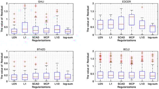
Figure 4.
The value of residual () on different datasets.
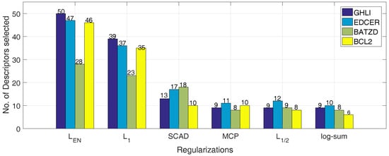
Figure 5.
The number of descriptors obtained by the multiple linear regression with the different penalties on different datasets(different colors represent different datasets).
First of all, in Table 6, Table 7, Table 8 and Table 9, the number of top-ranked informative descriptors identified by , , SCAD, MCP, and log-sum is 9, 10, 8 and 6 based on the value of the coefficients. Secondly, the common descriptors are emphasized in bold. Thirdly, as shown in Table 10, the number of descriptors is from the class of 2D. Then, the majority of descriptors are belong to the atom-type electrotopological state and autocorrelation of descriptors types. Finally, the name of the descriptors obtained by the log-sum method is exhibited in Table 11.
Table 6.
The 9 top-ranked descriptors identified by , , SCAD, MCP, and log-sum from the GHLI dataset (the common descriptors are emphasized in bold).
Table 7.
The 10 top-ranked descriptors identified by , , SCAD, MCP, and log-sum from the EDCER dataset (the common descriptors are emphasized in bold).
Table 8.
The 8 top-ranked descriptors identified by , , SCAD, MCP, and log-sum from the BATZD dataset (the common descriptors are emphasized in bold).
Table 9.
The 6 top-ranked descriptors identified by , , SCAD, MCP, and log-sum from the BCL2 dataset (the common descriptors are emphasized in bold).
Table 10.
The detailed information of the descriptors obtained by the log-sum method.
Table 11.
The name of the descriptors obtained by the log-sum method.
4. Conclusions
In the field of drug design and discovery, only a few descriptors are of interest to the QSAR model. Therefore, descriptor selection plays an important role in the study of QSAR. In this paper, we proposed univariate log-sum thresholding for updating the estimated coefficients and developed a coordinate descent algorithm for log-sum penalized multiple linear regression.
Both experimental results on artificial and four QSAR datasets demonstrate that our proposed multiple linear regression with log-sum penalty is still better than , , SCAD, MCP and . Therefore, our proposed log-sum method is the effective technique in both descriptor selection and prediction of biological activity.
In this paper, we introduced random sampling, which is easy to use, for QSAR data preprocessing. However, this method does not take into account additional knowledge. Therefore, we plan to integrate a self-paced learning mechanism, which learns easy samples first and then gradually takes into consideration complex samples, making the model more and more mature, with our proposed method in future work.
Acknowledgments
This work was supported by the Macau Science and Technology Development Funds from the Macau Special Administrative Region of the People’s Republic of China, the National Grand Fundamental Research 973 Program of China under Grant No. 2013CB329404 and the China NSFC projects under Contracts 61373114, 61661166011, 11690011, 61721002.
Author Contributions
Liang-Yong Xia, Hua Chai and Yong Liang designed the simulations. Liang-Yong Xia and De-Yu Meng provided the mathematical proof. Liang-Yong Xia, Xiao-Jun Yao and Yu-Wei Wang contributed to collecting the datasets and analyze the data. Liang-Yong Xia and Yong Liang designed and implemented the algorithm. Liang-Yong Xia, Yu-Wei Wang, De-Yu Meng, Xiao-Jun Yao and Yong Liang contributed to the interpretation of the results. Liang-Yong Xia took the lead in writing the manuscript. Yu-Wei Wang, De-Yu Meng, Xiao-Jun Yao, Hua Chai and Yong Liang revised the manuscript.
Conflicts of Interest
The authors declare no conflict of interest.
Abbreviations
| QSAR | Quantitative structure-activity relationship |
| QSRR | Quantitative structure-(chromatographic) retention relationships |
| QSPR | Quantitative structure-property relationship |
| QSTR | Quantitative structure-toxicity relationship |
| MLR | Multiple linear regression |
| MCP | Maximum concave penalty |
| SCAD | Smoothly clipped absolute deviation |
| LASSO | |
| BTAZD | (Benzo-)Triazoles toxicity in Daphnia magna |
| EDCER | EDC estrogen receptor binding |
| GHLI | Global half-life index |
| BCL2 | Apoptosis regulator Bcl-2 |
Appendix A. Proof
We first consider the situation :
Based on Equation (A1), the gradient of the log-sum regularization at can be expressed as:
Denote , , , which is equivalent to:
let: , Thus, we have:
Thus, , and it is then easy to obtain that when or and when . Therefore, Equation (16) has a local minimum. For , we can prove it in a similar way.
References
- Katritzky, A.R.; Kuanar, M.; Slavov, S.; Hall, C.D.; Karelson, M.; Kahn, I.; Dobchev, D.A. Quantitative correlation of physical and chemical properties with chemical structure: Utility for prediction. Chem. Rev. 2010, 110, 5714–5789. [Google Scholar] [CrossRef] [PubMed]
- Shahlaei, M. Descriptor selection methods in quantitative structure-activity relation-ship studies: A review study. Chem. Rev. 2013, 113, 8093–8103. [Google Scholar] [CrossRef] [PubMed]
- Liu, S.-S.; Liu, H.-L.; Yin, C.-S.; Wang, L.-S. Vsmp: A novel variable selection and modeling method based on the prediction. J. Chem. Inf. Comput. Sci. 2003, 43, 964–969. [Google Scholar] [CrossRef] [PubMed]
- Xu, L.; Zhang, W.-J. Comparison of different methods for variable selection. Anal. Chim. Acta 2001, 446, 475–481. [Google Scholar] [CrossRef]
- Wegner, J.K.; Zell, A. Prediction of aqueous solubility and partition coefficient optimized by a genetic algorithm based descriptor selection method. J. Chem. Inf. Comput. Sci. 2003, 43, 1077–1084. [Google Scholar] [CrossRef] [PubMed]
- Khajeh, A.; Modarress, H.; Zeinoddini-Meymand, H. Modified particle swarm optimization method for variable selection in qsar/qspr studies. Struct. Chem. 2013, 24, 1401–1409. [Google Scholar] [CrossRef]
- Meissner, M.; Schmuker, M.; Schneider, G. Optimized particle swarm optimization (OPSO) and its application to artificial neural network training. BMC Bioinform. 2006, 7, 125. [Google Scholar] [CrossRef] [PubMed]
- Ghosh, P.; Bagchi, M. QSAR modeling for quinoxaline derivatives using genetic algorithm and simulated annealing based feature selection. Curr. Med. Chem. 2009, 16, 4032–4048. [Google Scholar] [CrossRef] [PubMed]
- Burden, F.; Winkler, D. Bayesian regularization of neural networks. Artif. Neural Netw. Methods Appl. 2009, 458, 23–42. [Google Scholar]
- Dorigo, M.; Birattari, M.; Stutzle, T. Ant colony optimization. IEEE Comput. Intell. Mag. 2006, 1, 28–39. [Google Scholar] [CrossRef]
- Zheng, W.; Tropsha, A. Novel variable selection quantitative structure- property relationship approach based on the k-nearest-neighbor principle. J. Chem. Inf. Comput. Sci. 2000, 40, 185–194. [Google Scholar] [CrossRef] [PubMed]
- Mercader, A.G.; Duchowicz, P.R.; Fern’andez, F.M.; Castro, E.A. Modified and enhanced replacement method for the selection of molecular descriptors in qsar and qspr theories. Chemom. Intell. Lab. Syst. 2008, 92, 138–144. [Google Scholar] [CrossRef]
- Ara’ujo, M.C.U.; Saldanha, T.C.B.; Galvao, R.K.H.; Yoneyama, T.; Chame, H.C.; Visani, V. The successive projections algorithm for variable selection in spectroscopic multicomponent analysis. Chemom. Intell. Lab. Syst. 2001, 57, 65–73. [Google Scholar] [CrossRef]
- Put, R.; Daszykowski, M.; Baczek, T.; Heyden, Y.V. Retention prediction of peptides based on uninformative variable elimination by partial least squares. J. Proteome Res. 2006, 5, 1618–1625. [Google Scholar] [CrossRef] [PubMed]
- Daghir-Wojtkowiak, E.; Wiczling, P.; Bocian, S.; Kubik, L.; Koslinski, P.; Buszewski, B.; Kaliszan, R.; Markuszewski, M.J. Least absolute shrinkage and selection operator and dimensionality reduction techniques in quantitative structure retention relationship modeling of retention in hydrophilic interaction liquid chromatography. J. Chromatogr. A 2015, 1403, 54–62. [Google Scholar] [CrossRef] [PubMed]
- Goodarzi, M.; Chen, T.; Freitas, M.P. QSPR predictions of heat of fusion of organic compounds using Bayesian regularized artificial neural networks. Chemom. Intell. Lab. Syst. 2010, 104, 260–264. [Google Scholar] [CrossRef]
- Aalizadeh, R.; Peter, C.; Thomaidis, N.S. Prediction of acute toxicity of emerging contaminants on the water flea Daphnia magna by Ant Colony Optimization-Support Vector Machine QSTR models. Environ. Sci. Process. Impacts 2017, 19, 438–448. [Google Scholar] [CrossRef] [PubMed]
- Tibshirani, R. Regression shrinkage and selection via the lasso. J. R. Stat. Soc. Ser. B (Methodol.) 1996, 73, 267–288. [Google Scholar]
- Algamal, Z.; Lee, M. A new adaptive l1-norm for optimal descriptor selection of high-dimensional qsar classification model for anti-hepatitis c virus activity of thiourea derivatives. SAR QSAR Environ. Res. 2017, 28, 75–90. [Google Scholar] [CrossRef] [PubMed]
- Xu, Z.; Chang, X.; Xu, F.; Zhang, H. l1/2 regularization: A thresholding repre-sentation theory and a fast solver. IEEE Trans. Neural Netw. Learn. Syst. 2012, 23, 1013–1027. [Google Scholar] [PubMed]
- Algamal, Z.; Lee, M.; Al-Fakih, A.; Aziz, M. High-dimensional qsar modeling using penalized linear regression model with l1/2-norm. SAR QSAR Environ. Res. 2016, 27, 703–719. [Google Scholar] [CrossRef] [PubMed]
- Liang, Y.; Liu, C.; Luan, X.-Z.; Leung, K.-S.; Chan, T.-M.; Xu, Z.B.; Zhang, H. Sparse logistic regression with a l1/2 penalty for gene selection in cancer classification. BMC Bioinform. 2013, 14, 198. [Google Scholar] [CrossRef] [PubMed]
- Candes, E.J.; Wakin, M.B.; Boyd, S.P. Enhancing sparsity by reweighted l1 minimization. J. Fourier Anal. Appl. 2008, 14, 877–905. [Google Scholar] [CrossRef]
- Zou, H.; Hastie, T. Regularization and variable selection via the elastic net. J. R. Stat. Soc. Ser. B (Stat. Methodol.) 2005, 67, 301–320. [Google Scholar] [CrossRef]
- Donoho, D.L.; Johnstone, I.M. Ideal spatial adaptation by wavelet shrinkage. Biometrika 1994, 81, 425–455. [Google Scholar] [CrossRef]
- Fan, J.; Li, R. Variable selection via nonconcave penalized likelihood and its oracle properties. J. Am. Stat. Assoc. 2001, 96, 1348–1360. [Google Scholar] [CrossRef]
- Zhang, C.-H. Nearly unbiased variable selection under minimax concave penalty. Ann. Stat. 2010, 38, 894–942. [Google Scholar] [CrossRef]
- Gramatica, P.; Papa, E. Screening and ranking of pops for global half-life: Qsar approaches for prioritization based on molecular structure. Environ. Sci. Technol. 2007, 41, 2833–2839. [Google Scholar] [CrossRef] [PubMed]
- Li, J.; Gramatica, P. The importance of molecular structures, endpoints values, and predictivity parameters in qsar research: Qsar analysis of a series of estrogen receptor binders. Mol. Divers. 2010, 14, 687–696. [Google Scholar] [CrossRef] [PubMed]
- Cassani, S.; Kovarich, S.; Papa, E.; Roy, P.P.; van der Wal, L.; Gramatica, P. Daphnia and fish toxicity of (benzo) triazoles: Validated qsar models, and interspecies quantitative activity-activity modeling. J. Hazard. Mater. 2013, 258, 50–60. [Google Scholar] [CrossRef] [PubMed]
- Zakharov, A.V.; Peach, M.L.; Sitzmann, M.; Nicklaus, M.C. Qsar modeling of imbalanced high-throughput screening data in pubchem. J. Chem. Inf. Model. 2014, 54, 705–712. [Google Scholar] [CrossRef] [PubMed]
- Gramatica, P.; Cassani, S.; Chirico, N. QSARINS-Chem: Insubria Datasets and New QSAR/QSPR Models for Environmental Pollutants in QSARINS. J. Comput. Chem. Softw. News Updates 2014, 35, 1036–1044. [Google Scholar] [CrossRef] [PubMed]
- Golbraikh, A.; Tropsha, A. Beware of q2. J. Mol. Graph. Model. 2002, 20, 269–276. [Google Scholar] [CrossRef]
© 2017 by the authors. Licensee MDPI, Basel, Switzerland. This article is an open access article distributed under the terms and conditions of the Creative Commons Attribution (CC BY) license (http://creativecommons.org/licenses/by/4.0/).