
Incorporating Domain Knowledge and Structure-Based Descriptors for Machine Learning: A Case Study of Pd-Catalyzed Sonogashira Reactions


Abstract
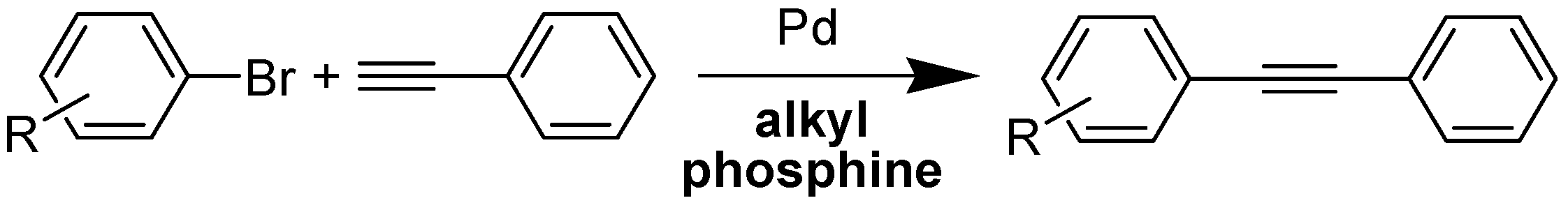
1. Introduction
2. Results
2.1. Performance of Our Ligand Descriptors
2.2. Comparison to Other Ligand Descriptors
2.3. Cross-Validation
3. Discussion
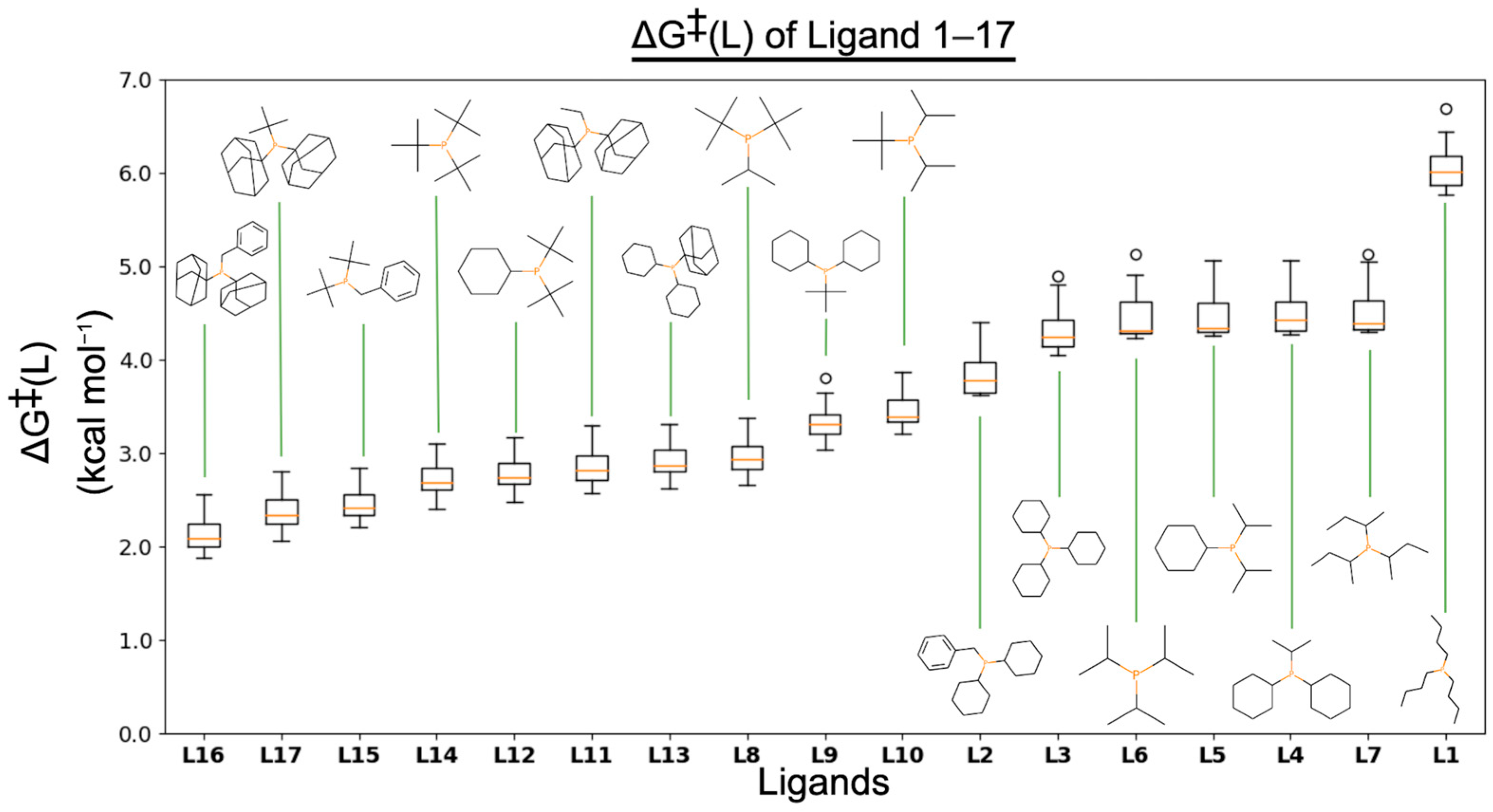
3.1. ΔG‡(L)
3.2. ΔG‡(L-S)
3.3. ΔG‡
4. Methodology
4.1. Descriptors
4.1.1. Descriptors for Aryl Bromides
4.1.2. Descriptors for Phosphine Ligands
4.2. Machine Learning
4.2.1. Machine Learning Architecture
4.2.2. Machine Learning Model Training Process
5. Computational Details
- Phosphine ligand descriptors were passed through a GNN layer with 3–5 iterations in which each iteration had the same weight without bias. The GNN layer was constructed in the framework of a message-passing neural network (MPNN) using Leaky ReLU activation with a = 0.01, size 2–4 for message function, and size 1 for update function. The graphical output was concatenated according to the order of an aligned graph. The generated vector was referred to as GNN Output States.
- Aryl bromide descriptors and GNN Output States were concatenated and passed through a fully connected neural network (FCNN) layer using Sigmoid activation, size 1, L2-regularizer, and no bias. The generated vector was referred to as Hidden States 1.
- GNN Output States were passed through an FCNN layer using Sigmoid activation, size 1, L2-regularizer, with non-negative weights and no bias. The generated vector was referred to as Hidden States 2.
- Hidden States 1 and Hidden States 2 were passed through an FCNN layer using linear activation, size 1, with non-negative weights and no bias, generating predicted activation energies.
- Predicted activation energies were converted to reaction rate constants using the Eyring equation.
6. Conclusions
Supplementary Materials
Author Contributions
Funding
Institutional Review Board Statement
Informed Consent Statement
Data Availability Statement
Acknowledgments
Conflicts of Interest
Sample Availability
References
- Jordan, M.I.; Mitchell, T.M. Machine learning: Trends, perspectives, and prospects. Science 2015, 349, 255–260. [Google Scholar] [CrossRef] [PubMed]
- Tu, J.V. Advantages and disadvantages of using artificial neural networks versus logistic regression for predicting medical outcomes. J. Clin. Epidemiol. 1996, 49, 1225–1231. [Google Scholar] [CrossRef] [PubMed]
- Zanardi, M.M.; Sarotti, A.M. GIAO C–H COSY Simulations Merged with Artificial Neural Networks Pattern Recognition Analysis. Pushing the Structural Validation a Step Forward. J. Org. Chem. 2015, 80, 9371–9378. [Google Scholar] [CrossRef] [PubMed]
- Mansouri, K.; Cariello, N.F.; Korotcov, A.; Tkachenko, V.; Grulke, C.M.; Sprankle, C.S.; Allen, D.; Casey, W.M.; Kleinstreuer, N.C.; Williams, A.J. Open-source QSAR models for pKa prediction using multiple machine learning approaches. J. Cheminform. 2019, 11, 60. [Google Scholar] [CrossRef] [PubMed]
- Yang, Q.; Li, Y.; Yang, J.D.; Liu, Y.; Zhang, L.; Luo, S.; Cheng, J.P. Holistic Prediction of the pKa in Diverse Solvents Based on a Machine-Learning Approach. Angew. Chem. Int. Ed. Engl. 2020, 59, 19282–19291. [Google Scholar] [CrossRef]
- Ramakrishnan, R.; Dral, P.O.; Rupp, M.; von Lilienfeld, O.A. Big data meets quantum chemistry approximations: The Δ-machine learning approach. J. Chem. Theory Comput. 2015, 11, 2087–2096. [Google Scholar] [CrossRef]
- Unke, O.T.; Meuwly, M. PhysNet: A neural network for predicting energies, forces, dipole moments, and partial charges. J. Chem. Theory Comput. 2019, 15, 3678–3693. [Google Scholar] [CrossRef]
- von Lilienfeld, O.A. Quantum machine learning in chemical compound space. Angew. Chem. Int. Ed. Engl. 2018, 57, 4164–4169. [Google Scholar] [CrossRef]
- Rupp, M.; Tkatchenko, A.; Müller, K.R.; von Lilienfeld, O.A. Fast and accurate modeling of molecular atomization energies with machine learning. Phys. Rev. Lett. 2012, 108, 058301. [Google Scholar] [CrossRef]
- Gastegger, M.; Behler, J.; Marquetand, P. Machine learning molecular dynamics for the simulation of infrared spectra. Chem. Sci. 2017, 8, 6924–6935. [Google Scholar] [CrossRef]
- Montavon, G.; Rupp, M.; Gobre, V.; Vazquez-Mayagoitia, A.; Hansen, K.; Tkatchenko, A.; Müller, K.R.; von Lilienfeld, O.A. Machine learning of molecular electronic properties in chemical compound space. New J. Phys. 2013, 15, 095003. [Google Scholar] [CrossRef]
- Coley, C.W.; Barzilay, R.; Jaakkola, T.S.; Green, W.H.; Jensen, K.F. Prediction of Organic Reaction Outcomes Using Machine Learning. ACS Cent. Sci. 2017, 3, 434–443. [Google Scholar] [CrossRef]
- Coley, C.W.; Green, W.H.; Jensen, K.F. Machine Learning in Computer-Aided Synthesis Planning. Acc. Chem. Res. 2018, 51, 1281–1289. [Google Scholar] [CrossRef]
- Gómez-Bombarelli, R.; Aguilera-Iparraguirre, J.; Hirzel, T.D.; Duvenaud, D.; Maclaurin, D.; Blood-Forsythe, M.A.; Chae, H.S.; Einzinger, M.; Ha, D.G.; Wu, T.; et al. Design of efficient molecular organic light-emitting diodes by a high-throughput virtual screening and experimental approach. Nat. Mater. 2016, 15, 1120–1127. [Google Scholar] [CrossRef]
- Xie, T.; Grossman, J.C. Crystal Graph Convolutional Neural Networks for an Accurate and Interpretable Prediction of Material Properties. Phys. Rev. Lett. 2018, 120, 145301. [Google Scholar] [CrossRef]
- Coley, C.W.; Jin, W.; Rogers, L.; Jamison, T.F.; Jaakkola, T.S.; Green, W.H.; Barzilay, R.; Jensen, K.F. A graph-convolutional neural network model for the prediction of chemical reactivity. Chem. Sci. 2019, 10, 370–377. [Google Scholar] [CrossRef]
- Schwaller, P.; Vaucher, A.C.; Laino, T.; Reymond, J.L. Prediction of chemical reaction yields using deep learning. Mach. Learn. Sci. Technol. 2021, 2, 015016. [Google Scholar] [CrossRef]
- Schwaller, P.; Hoover, B.; Reymond, J.L.; Strobelt, H.; Laino, T. Unsupervised Attention-Guided Atom-Mapping. Sci. Adv. 2021, 7, eabe4166. [Google Scholar] [CrossRef]
- Ahneman, D.T.; Estrada, J.G.; Lin, S.; Dreher, S.D.; Doyle, A.G. Predicting reaction performance in C–N cross-coupling using machine learning. Science 2018, 360, 186–190. [Google Scholar] [CrossRef]
- Nielsen, M.K.; Ahneman, D.T.; Riera, O.; Doyle, A.G. Deoxyfluorination with Sulfonyl Fluorides: Navigating Reaction Space with Machine Learning. J. Am. Chem. Soc. 2018, 140, 5004–5008. [Google Scholar] [CrossRef]
- Yada, A.; Matsumura, T.; Ando, Y.; Nagata, K.; Ichinoseki, S.; Sato, K. Ensemble Learning Approach with LASSO for Predicting Catalytic Reaction Rates. Synlett 2021, 32, 1843–1848. [Google Scholar] [CrossRef]
- Zahrt, A.F.; Henle, J.J.; Rose, B.T.; Wang, Y.; Darrow, W.T.; Denmark, S.E. Prediction of higher-selectivity catalysts by computer-driven workflow and machine learning. Science 2019, 363, eaau5631. [Google Scholar] [CrossRef] [PubMed]
- Domingo, L.R.; Aurell, M.J.; Pérez, P.; Contreras, R. Quantitative characterization of the global electrophilicity power of common diene/dienophile pairs in Diels–Alder reactions. Tetrahedron 2002, 58, 4417–4423. [Google Scholar] [CrossRef]
- Teixeira, F.; Cordeiro, M.N.D. Simple descriptors for assessing the outcome of aza-Diels–Alder reactions. RSC Adv. 2015, 5, 50729–50740. [Google Scholar] [CrossRef]
- an der Heiden, M.R.; Plenio, H.; Immel, S.; Burello, E.; Rothenberg, G.; Hoefsloot, H.C.J. Insights into Sonogashira Cross-Coupling by High-Throughput Kinetics and Descriptor Modeling. Chem. Eur. J. 2008, 14, 2857–2866. [Google Scholar] [CrossRef]
- Gensch, T.; dos Passos Gomes, G.; Friederich, P.; Peters, E.; Gaudin, T.; Pollice, R.; Jorner, K.; Nigam, A.; Lindner-D’Addario, M.; Sigman, M.S.; et al. A comprehensive discovery platform for organophosphorus ligands for catalysis. J. Am. Chem. Soc. 2022, 144, 1205–1217. [Google Scholar] [CrossRef]
- Sandfort, F.; Strieth-Kalthoff, F.; Kühnemund, M.; Beecks, C.; Glorius, F. A structure-based platform for predicting chemical reactivity. Chem 2020, 6, 1379–1390. [Google Scholar] [CrossRef]
- Barrios-Landeros, F.; Hartwig, J.F. Distinct mechanisms for the oxidative addition of chloro-, bromo-, and iodoarenes to a bisphosphine palladium (0) complex with hindered ligands. J. Am. Chem. Soc. 2005, 127, 6944–6945. [Google Scholar] [CrossRef]
- Fleckenstein, C.A.; Plenio, H. Sterically demanding trialkylphosphines for palladium-catalyzed cross coupling reactions—Alternatives to PtBu3. Chem. Soc. Rev. 2010, 39, 694–711. [Google Scholar] [CrossRef]
- Schilz, M.; Plenio, H. A guide to Sonogashira cross-coupling reactions: The influence of substituents in aryl bromides, acetylenes, and phosphines. J. Org. Chem. 2012, 77, 2798–2807. [Google Scholar] [CrossRef]
- Barrios-Landeros, F.; Carrow, B.P.; Hartwig, J.F. Effect of ligand steric properties and halide identity on the mechanism for oxidative addition of haloarenes to trialkylphosphine Pd (0) complexes. J. Am. Chem. Soc. 2009, 131, 8141–8154. [Google Scholar] [CrossRef]
- Crabtree, R.H. The Organometallic Chemistry of the Transition Metals, 6th ed.; John Wiley & Sons: New York, NY, USA, 2014; pp. 163–203. [Google Scholar]
- Spessard, G.; Miessler, G. Euan Cameron. Organometallic Chemistry, 2nd ed.; Oxford University Press: New York, NY, USA, 2010; pp. 585–586. [Google Scholar]
- Labinger, J.A. Tutorial on oxidative addition. Organometallics 2015, 34, 4784–4795. [Google Scholar] [CrossRef]
- Xue, L.; Lin, Z. Theoretical aspects of palladium-catalysed carbon–carbon cross-coupling reactions. Chem. Soc. Rev. 2010, 39, 1692–1705. [Google Scholar] [CrossRef]
- Hammett, L.P. The effect of structure upon the reactions of organic compounds. Benzene derivatives. J. Am. Chem. Soc. 1937, 59, 96–103. [Google Scholar] [CrossRef]
- Masood, H.; Toe, C.Y.; Teoh, W.Y.; Sethu, V.; Amal, R. Machine Learning for Accelerated Discovery of Solar Photocatalysts. ACS Catal. 2019, 9, 11774–11787. [Google Scholar] [CrossRef]
- Zhou, Z.; Kearnes, S.; Li, L.; Zare, R.N.; Riley, P. Optimization of Molecules via Deep Reinforcement Learning. Sci. Rep. 2019, 9, 10752. [Google Scholar] [CrossRef]
- Miyaura, N.; Suzuki, A. Palladium-Catalyzed Cross-Coupling Reactions of Organoboron Compounds. Chem. Rev. 1995, 95, 2457–2483. [Google Scholar] [CrossRef]
- Nicolaou, K.C.; Bulger, P.G.; Sarlah, D. Palladium-Catalyzed Cross-Coupling Reactions in Total Synthesis. Angew. Chem. Int. Ed. Engl. 2005, 44, 4442–4489. [Google Scholar] [CrossRef]
- Abadi, M.; Agarwal, A.; Barham, P.; Brevdo, E.; Chen, Z.; Citro, C.; Corrado, G.S.; Davis, A.; Dean, J.; Devin, M.; et al. TensorFlow: Large-Scale Machine Learning on Heterogeneous Systems. 2015. Available online: https://tensorflow.org/ (accessed on 1 January 2021).
- Wang, M.; Yu, L.; Zheng, D.; Gan, Q.; Gai, Y.; Ye, Z.; Li, M.; Zhou, J.; Huang, Q.; Ma, C.; et al. Deep graph library: A graph-centric, highly-performant package for graph neural networks. arXiv 2019, arXiv:1909.01315. [Google Scholar]
- Akiba, T.; Sano, S.; Yanase, T.; Ohta, T.; Koyama, M. Optuna: A next-generation hyperparameter optimization framework. In Proceedings of the 25th ACM SIGKDD International Conference on Knowledge Discovery & Data Mining, Anchorage, AK, USA, 4–8 August 2019; Association for Computing Machinery: Anchorage, AK, USA, 2019; pp. 2623–2631. [Google Scholar]
- Perrin, D.D.; Dempsey, B.; Serjeant, E.P. pKa Prediction for Organic Acids and Bases; Springer: New York, NY, USA, 1981; pp. 109–126. [Google Scholar]


| Ligand Descriptor | Model | Training Set | Validation Set | Testing Set | |||
|---|---|---|---|---|---|---|---|
| R2 | MAE | R2 | MAE | R2 | MAE | ||
| Graphical Representation (i.e., our descriptor) | GNN | 0.94 | 0.81 | 0.87 | 1.04 | 0.84 | 1.15 |
| Buried Volume | FCNN | <0 | 3.500 | <0 | 3.233 | <0 | 3.508 |
| Restricted Linear Regression | 0.27 | 3.46 | 0.34 | 2.78 | 0.30 | 4.06 | |
| Cone Angle | FCNN | <0 | 3.500 | <0 | 3.233 | <0 | 3.508 |
| Restricted Linear Regression | 0.26 | 3.52 | 0.33 | 2.78 | 0.28 | 4.03 | |
| Buried Volume and Cone Angle | FCNN | <0 | 3.500 | <0 | 3.233 | <0 | 3.508 |
| Restricted Linear Regression | 0.27 | 3.46 | 0.34 | 2.78 | 0.30 | 4.06 | |
| One-Hot Encoding | FCNN | <0 | 3.502 | <0 | 3.232 | <0 | 3.511 |
| Restricted Linear Regression | 0.52 | 2.85 | 0.52 | 2.38 | 0.51 | 3.07 | |
| Multiple Fingerprint Features (MFF) | FCNN | <0 | 3.500 | <0 | 3.233 | <0 | 3.508 |
| Restricted Linear Regression | 0.52 | 2.85 | 0.52 | 2.38 | 0.51 | 3.07 | |
| Dataset | Cross-Validation Set Performance (R2) | Average Performance (R2) | |||
|---|---|---|---|---|---|
| Set 1 | Set 2 | Set 3 | Set 4 1 | ||
| Training Set | 0.94 | 0.93 | 0.91 | 0.92 | 0.93 |
| Validation Set | 0.87 | 0.76 | 0.78 | 0.93 | 0.84 |
| Testing Set | 0.84 | 0.87 | 0.87 | 0.91 | 0.87 |
Disclaimer/Publisher’s Note: The statements, opinions and data contained in all publications are solely those of the individual author(s) and contributor(s) and not of MDPI and/or the editor(s). MDPI and/or the editor(s) disclaim responsibility for any injury to people or property resulting from any ideas, methods, instructions or products referred to in the content. |
© 2023 by the authors. Licensee MDPI, Basel, Switzerland. This article is an open access article distributed under the terms and conditions of the Creative Commons Attribution (CC BY) license (https://creativecommons.org/licenses/by/4.0/).
Share and Cite
Chan, K.; Ta, L.T.; Huang, Y.; Su, H.; Lin, Z. Incorporating Domain Knowledge and Structure-Based Descriptors for Machine Learning: A Case Study of Pd-Catalyzed Sonogashira Reactions. Molecules 2023, 28, 4730. https://doi.org/10.3390/molecules28124730
Chan K, Ta LT, Huang Y, Su H, Lin Z. Incorporating Domain Knowledge and Structure-Based Descriptors for Machine Learning: A Case Study of Pd-Catalyzed Sonogashira Reactions. Molecules. 2023; 28(12):4730. https://doi.org/10.3390/molecules28124730
Chicago/Turabian StyleChan, Kalok, Long Thanh Ta, Yong Huang, Haibin Su, and Zhenyang Lin. 2023. "Incorporating Domain Knowledge and Structure-Based Descriptors for Machine Learning: A Case Study of Pd-Catalyzed Sonogashira Reactions" Molecules 28, no. 12: 4730. https://doi.org/10.3390/molecules28124730
APA StyleChan, K., Ta, L. T., Huang, Y., Su, H., & Lin, Z. (2023). Incorporating Domain Knowledge and Structure-Based Descriptors for Machine Learning: A Case Study of Pd-Catalyzed Sonogashira Reactions. Molecules, 28(12), 4730. https://doi.org/10.3390/molecules28124730