
Unveiling the Molecular Origin of Vapor-Liquid Phase Transition of Bulk and Confined Fluids

 , ,
, ,
Abstract
:1. Introduction
2. Results and Discussion
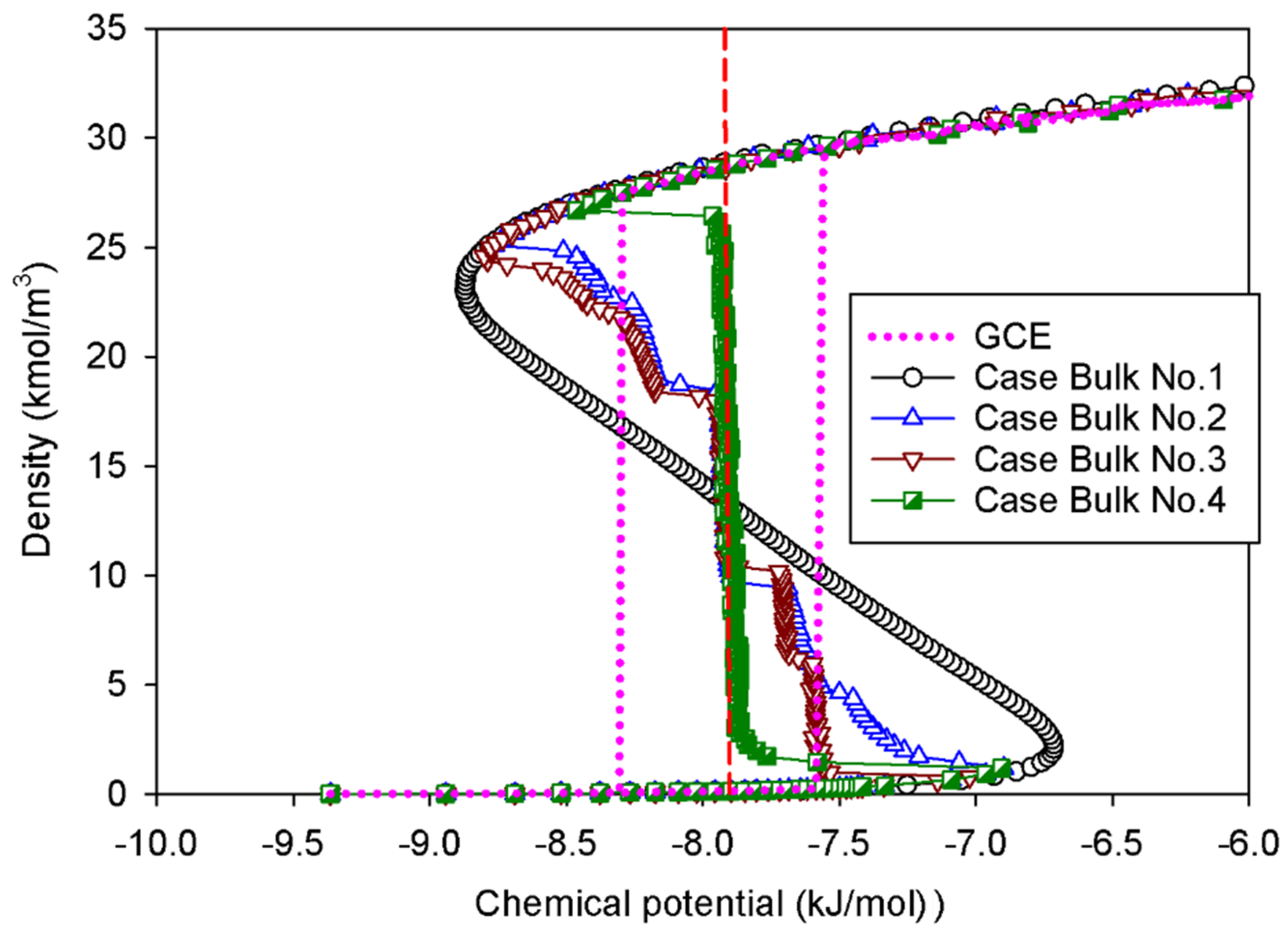
2.1. Vapor–Liquid Phase Transition of Nitrogen in the Bulk Phase
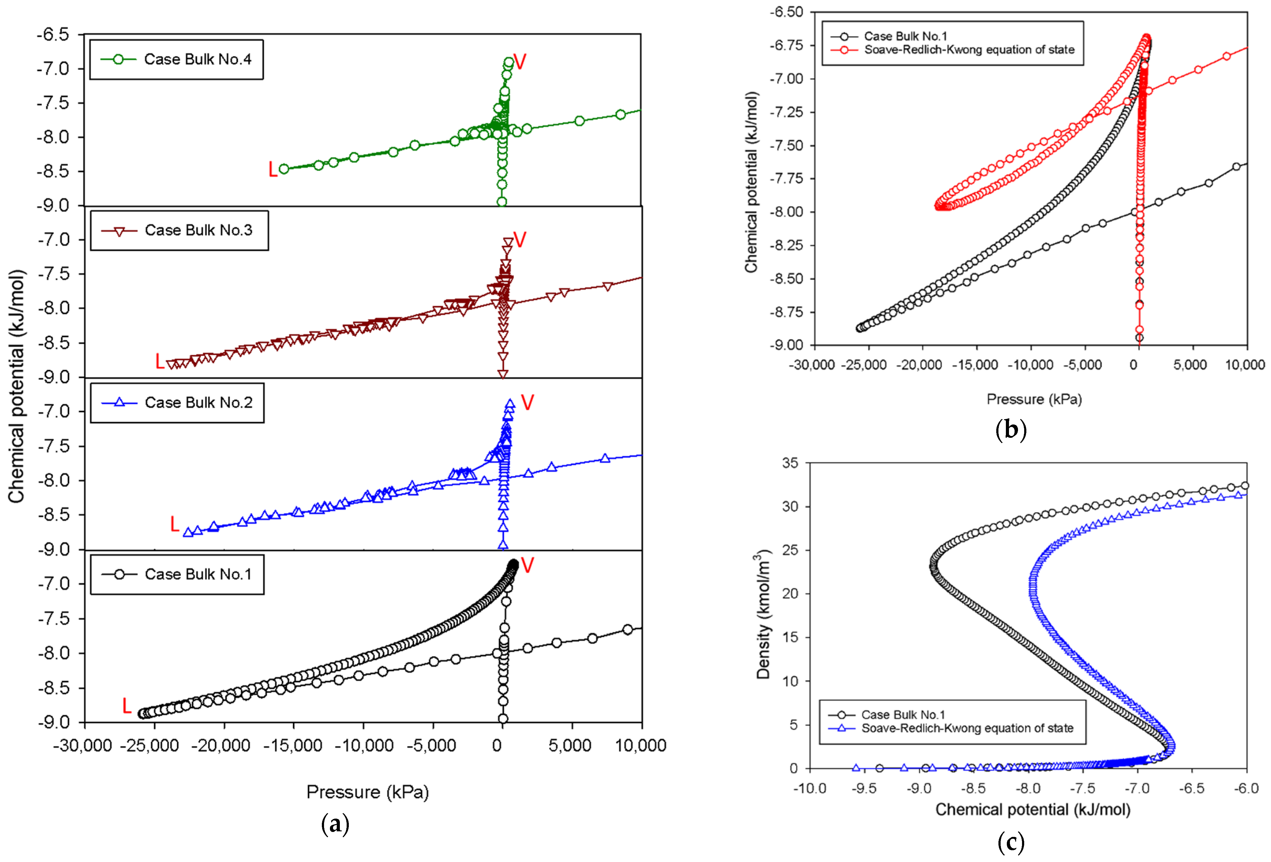
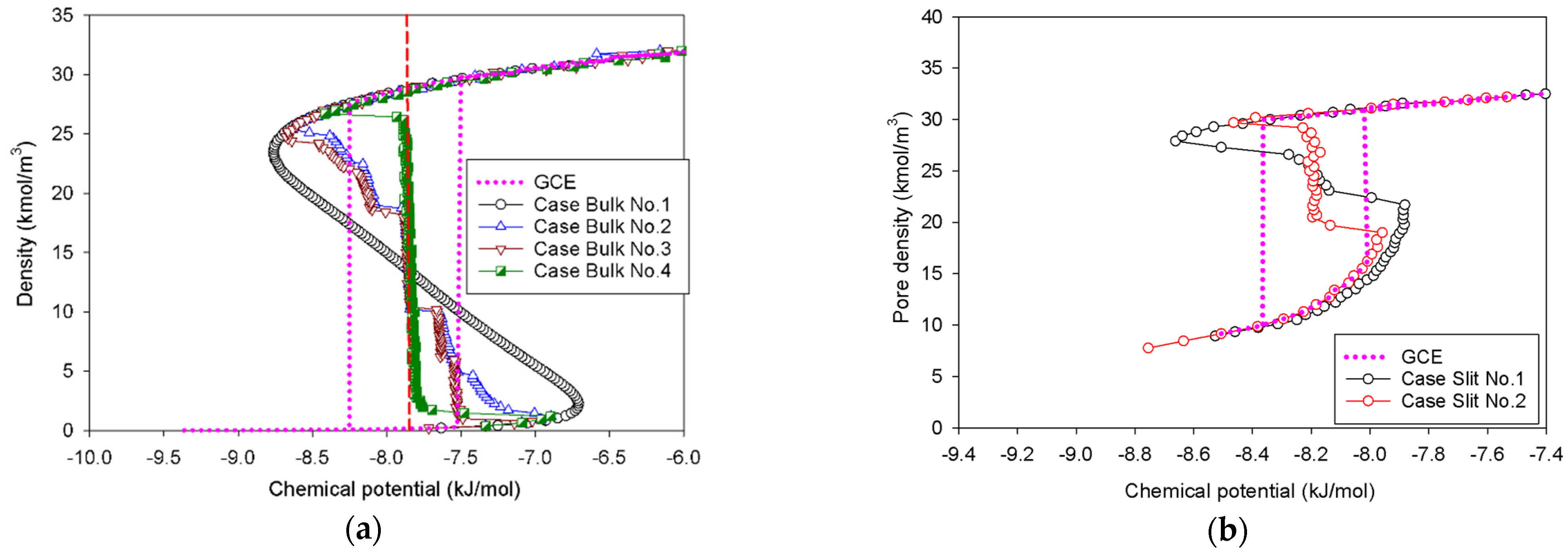
2.1.1. Group I: Smooth S-Shaped Isotherm
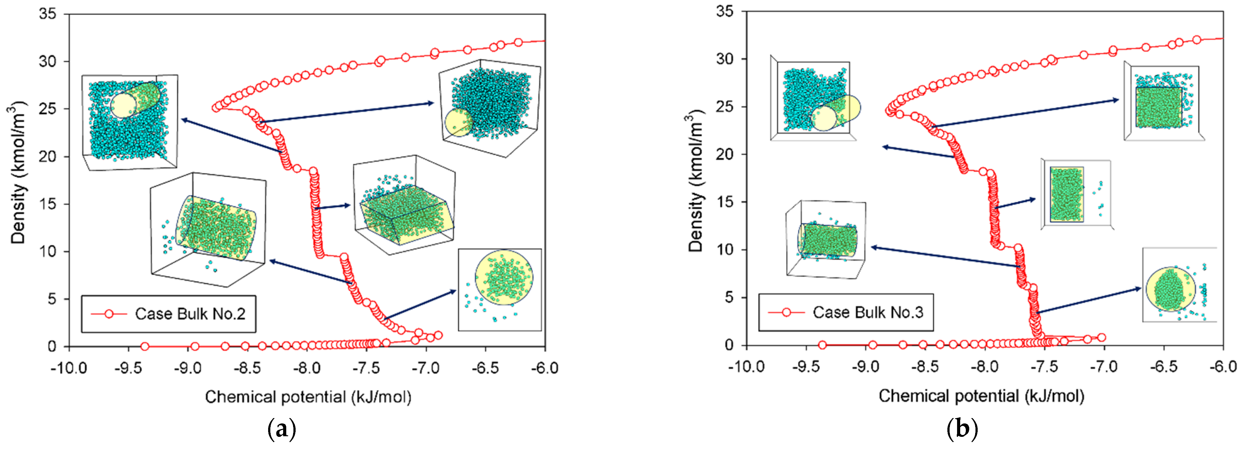
2.1.2. Group II: Stepwise S-Shaped Isotherm
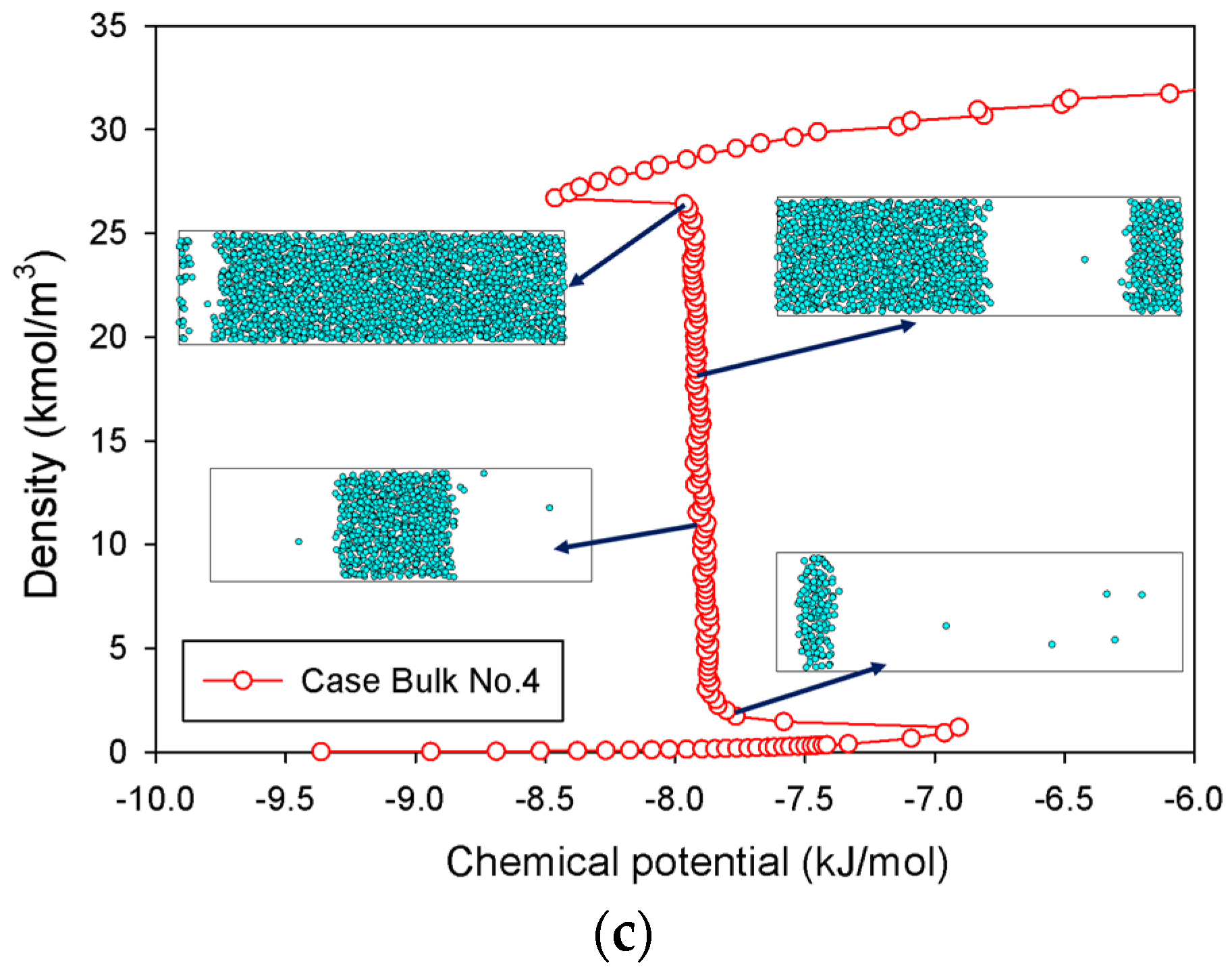
2.1.3. Group III: Stepwise S-Shaped Isotherm with Just a Vertical Segment
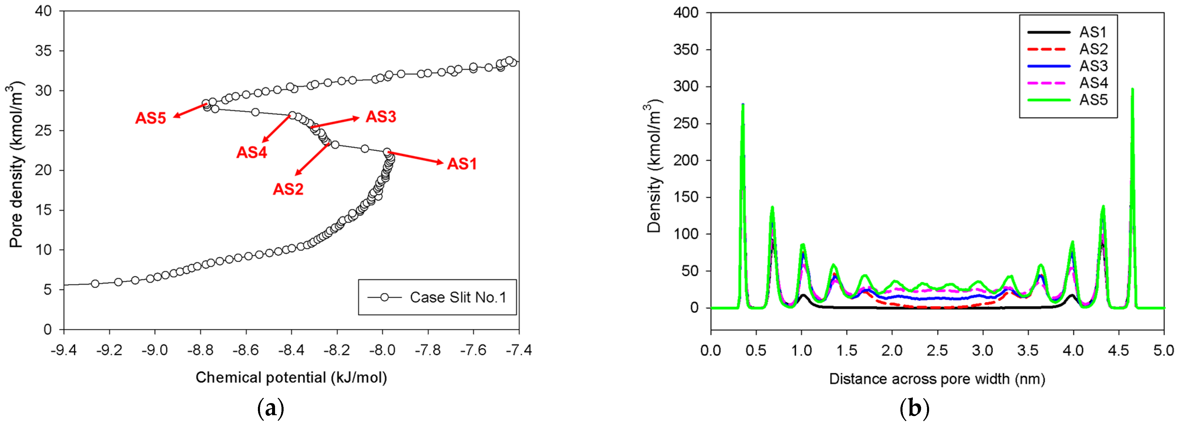
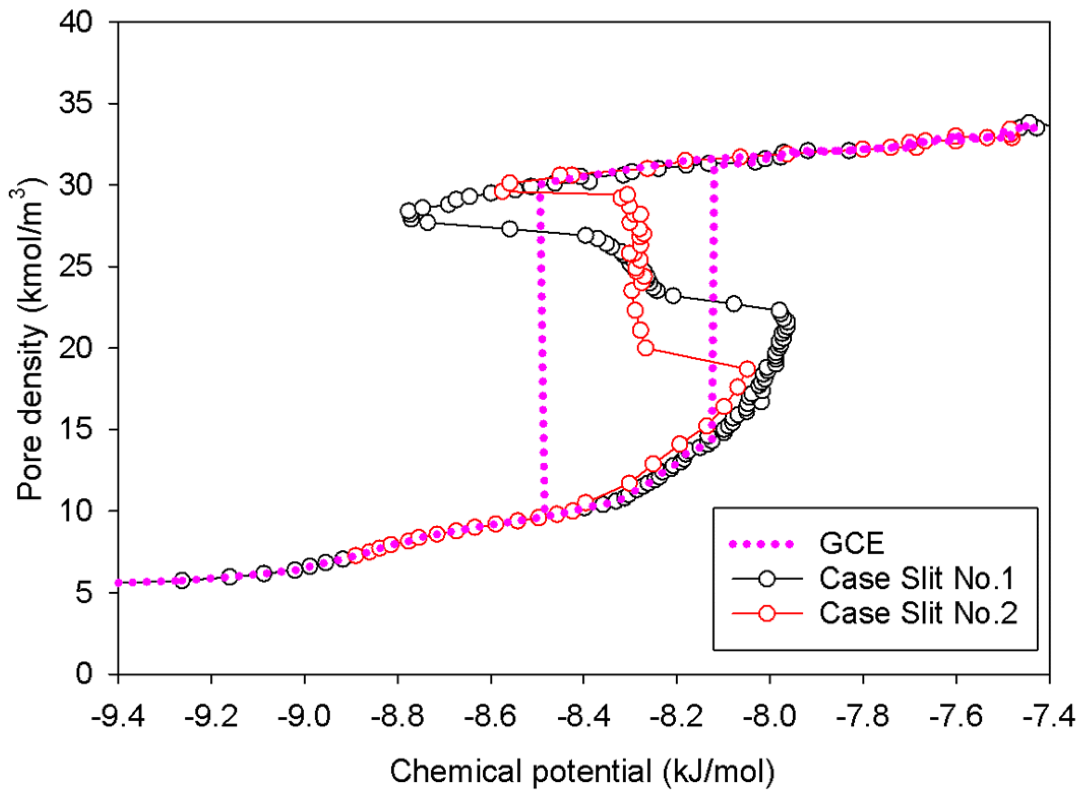
2.2. Nitrogen Adsorption in the Infinite Slit Mesopore
- (1)
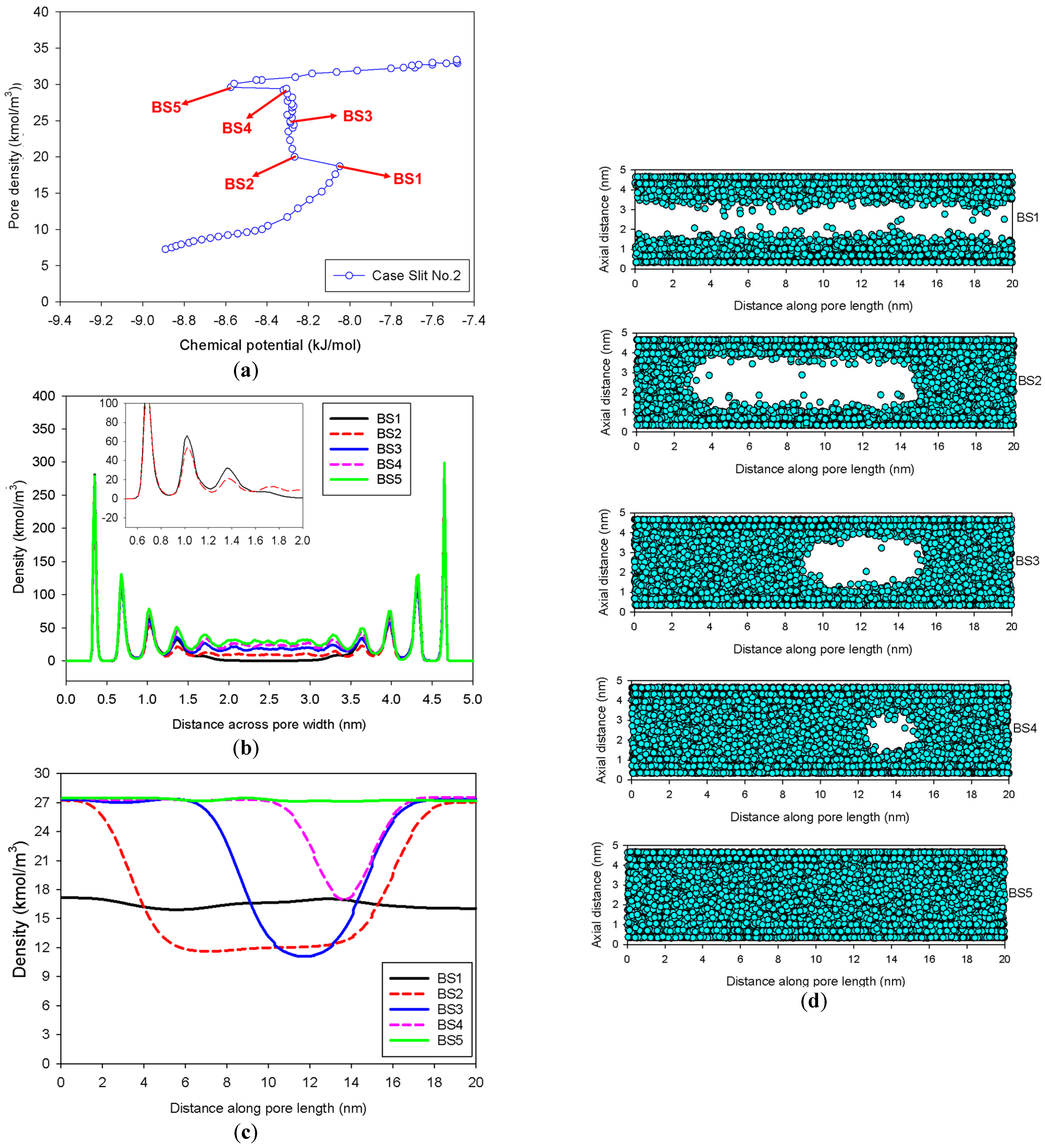
- At Point BS1 of Figure 6c, the threshold density of the metastable adsorbed layers is about 17 kmol/m3, where the adsorbed films on opposite pore walls are close enough to create a liquid bridge.
- (2)
- At Point BS2 of Figure 6c, this is the process of nucleation of a liquid bridge at the coexistence chemical potential [37]. The densities of stable adsorbed layers and the liquid embryo are approximately 12 and 27 kmol/m3, respectively. The liquid bridge has two concave cylindrical menisci, which indicate the reduction of chemical potential.
- (3)
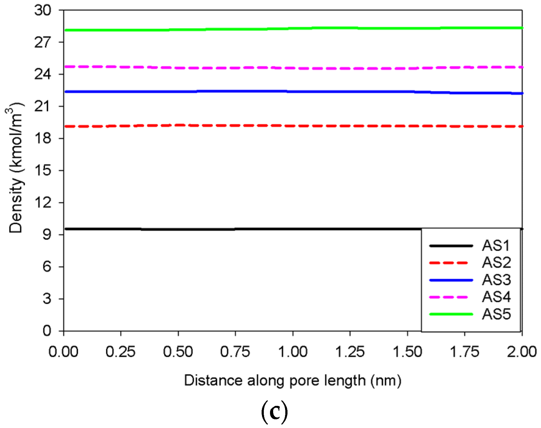
- The creation of a liquid bridge between Points BS1 and BS2 is mostly due to a decrease in density in the second and third adsorbed layers (as shown in the inset of Figure 6b). This is why the density of stable adsorbed layers is lower than that of the metastable adsorbed layers.
- (4)
- The axial density of the metastable adsorbed layer at Point BS1 is noticeably higher than at Point AS1, indicating that the surface dimension of the carbon substrate for Slit No.1 is insufficient to construct the liquid bridge.
- (5)
- The density at Point BS1 is greater than that at the point just before sudden condensation of the GCE isotherm. This is because the minute size of the dosing cell used in the MCE simulation allows the adsorption system to control a much narrower undulating zone between the adsorbed layers and the gas-like core to be substantially smaller [38], requiring a greater chemical potential to build up the adsorbed layer for condensation.
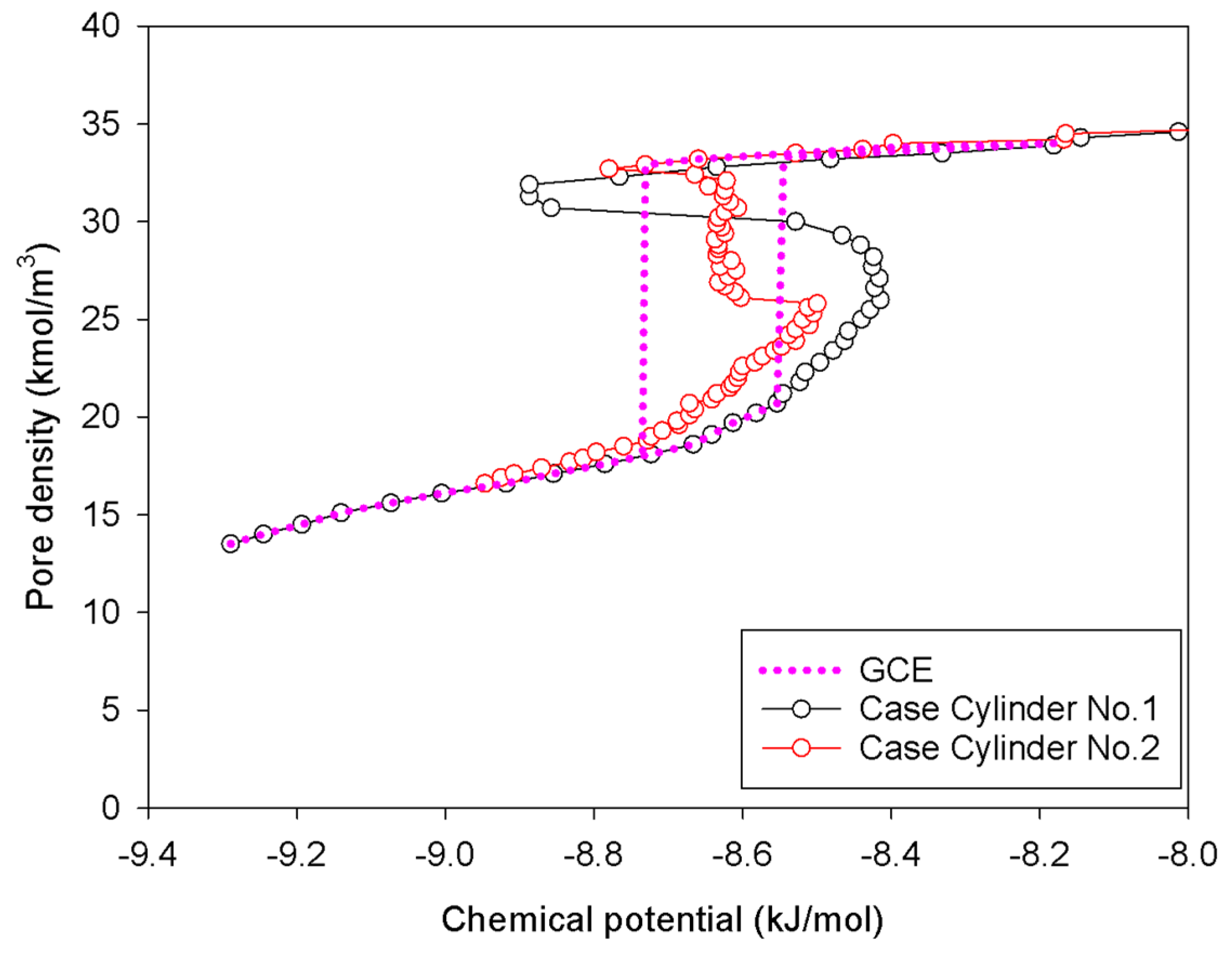
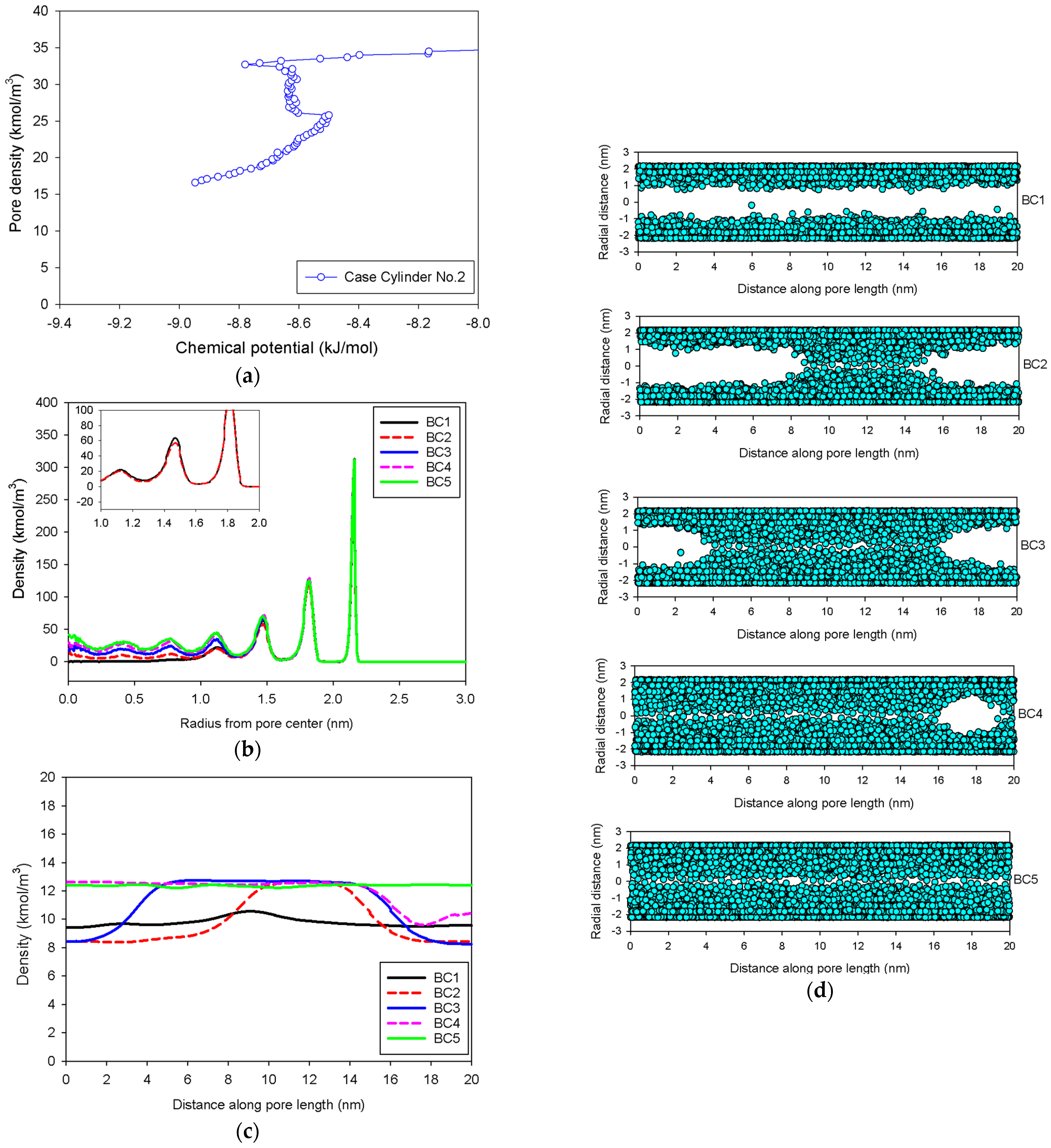
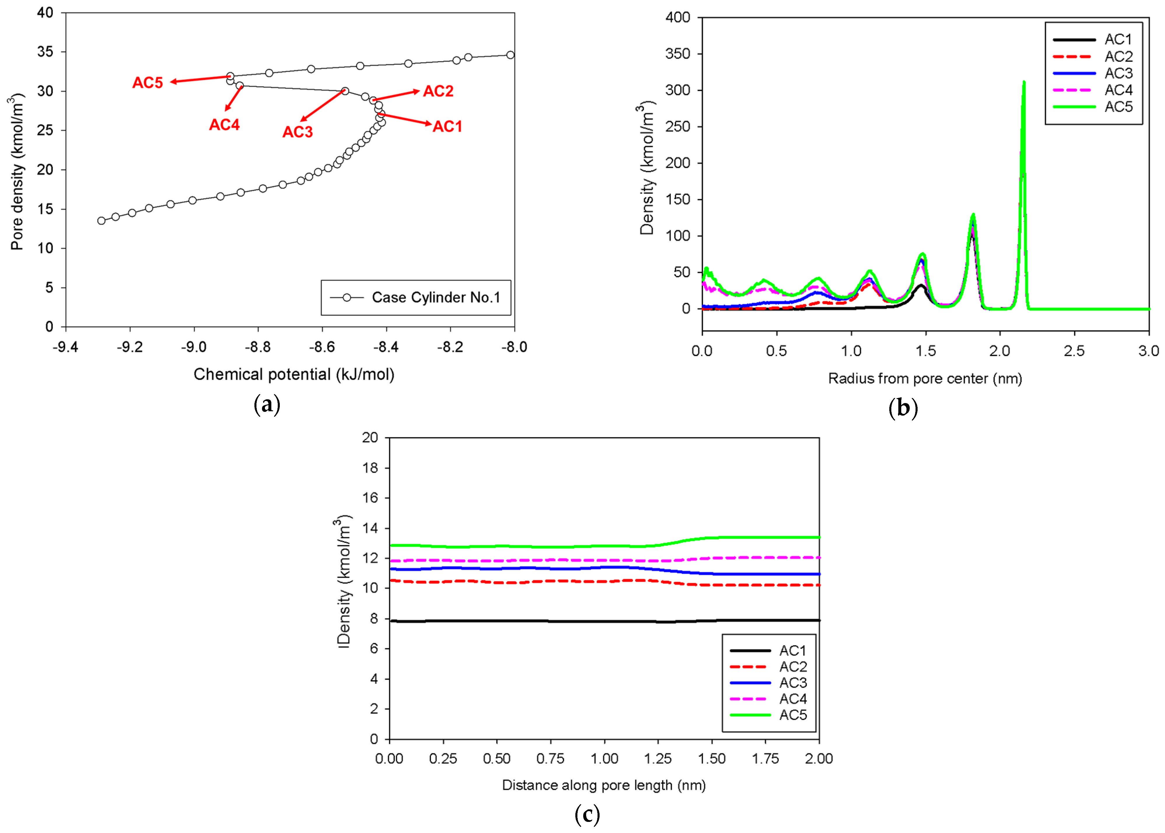
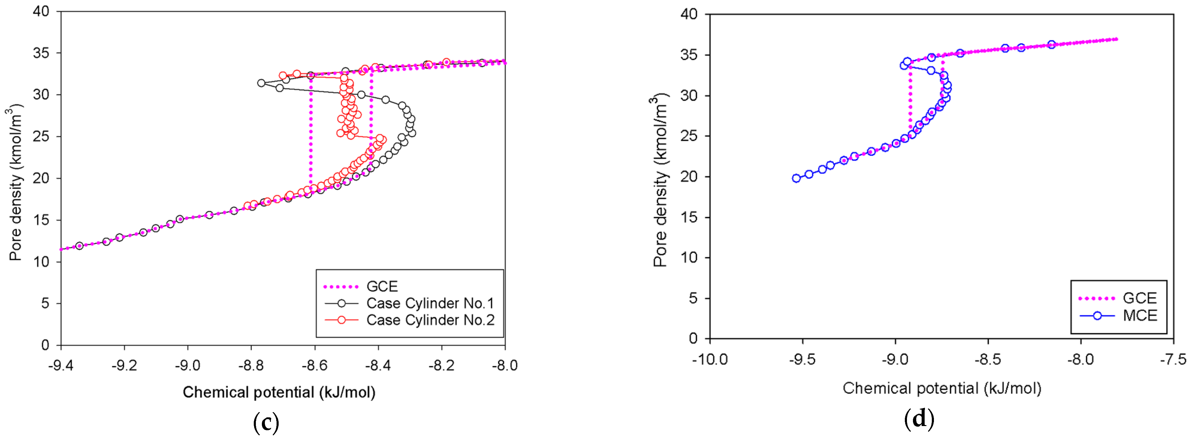
2.3. Nitrogen Adsorption in the Infinite Cylindrical Mesopore
- (1)
- Adsorption progresses up to Point BC1 via the formation of cylindrical interfacial curvature by the accumulation of metastable adsorbed layers across the radial direction (Figure 9b).
- (2)
- The curvature of the interface changes from cylinder to hemispheres during the formation of the liquid bridge by supplying molecules from the second adsorbed layer (Point BC2 in Figure 9b). This differs from what we found in the slit pore, where the interfacial curvature ranges from two parallel slabs to semi-cylindrical menisci.
- (3)
- All spinodal points and the equilibrium phase transition occur at a lower chemical potential than in slit pore; this is attributed to the larger curvature of the interface suppressing the size of the undulating interface [41]. For a given pore size, the condensation in a cylinder requires fewer adsorbed layers than in a slit pore, and the core size in a cylinder just before capillary condensation is greater than in a slit pore.
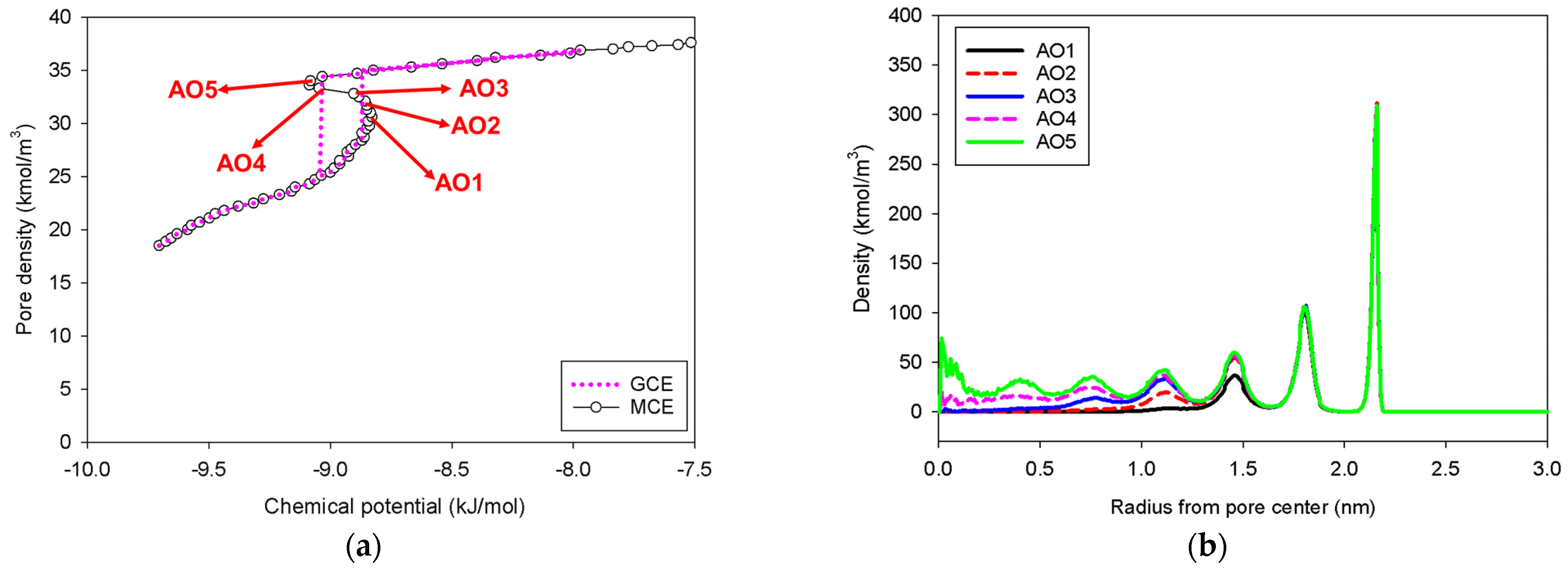
2.4. Nitrogen Adsorption in the Spherical Mesopore
2.5. Effect of Molecular Model of Nitrogen
3. Materials and Methods
3.1. Fluid–Fluid Interaction Models
3.2. Solid–Fluid Interaction Models
3.3. Monte Carlo Simulations
4. Conclusions
Author Contributions
Funding
Institutional Review Board Statement
Informed Consent Statement
Data Availability Statement
Acknowledgments
Conflicts of Interest
References
- Kontogeorgis, G.M.; Dohrn, R.; Economou, I.G.; de Hemptinne, J.-C.; Kate, A.T.; Kuitunen, S.; Mooijer, M.; Žilnik, L.F.; Vesovic, V. Industrial Requirements for Thermodynamic and Transport Properties: 2020. Ind. Eng. Chem. Res. 2021, 60, 4987–5013. [Google Scholar] [CrossRef] [PubMed]
- Campbell, F.C. Phase Diagrams: Understanding the Basics; ASM International: Materials Park, OH, USA, 2012. [Google Scholar]
- Greiner, W.; Neise, L.; Stöcker, H. Classification of Phase Transitions. In Thermodynamics and Statistical Mechanics; Springer: New York, NY, USA, 1995; pp. 416–435. [Google Scholar]
- Binder, K. Theory of first-order phase transitions. Rep. Prog. Phys. 1987, 50, 783. [Google Scholar] [CrossRef]
- Stishov, S.M.; Petrova, A.E. Critical Points and Phase Transitions. J. Exp. Theor. Phys. 2020, 131, 1056–1063. [Google Scholar] [CrossRef]
- Daub, E.E. Gibbs phase rule: A centenary retrospect. J. Chem. Educ. 1976, 53, 747. [Google Scholar] [CrossRef]
- Gutiérrez, G. Gibbs’ phase rule revisited. Theor. Math. Phys. 1996, 108, 1222–1224. [Google Scholar] [CrossRef]
- Forero, L.A.; Velásquez, J.A. A generalized cubic equation of state for non-polar and polar substances. Fluid Phase Equilib. 2016, 418, 74–87. [Google Scholar] [CrossRef]
- Kontogeorgis, G.M.; Privat, R.; Jaubert, J.-N. Taking Another Look at the van der Waals Equation of State—Almost 150 Years Later. J. Chem. Eng. Data 2019, 64, 4619–4637. [Google Scholar] [CrossRef] [Green Version]
- Rajendran, K.; Ravi, R. Critical Analysis of Maxwell’s Equal Area Rule: Implications for Phase Equilibrium Calculations. Ind. Eng. Chem. Res. 2010, 49, 7687–7692. [Google Scholar] [CrossRef]
- Zhao, D.; Yu, K.; Han, X.; He, Y.; Chen, B. Recent progress on porous MOFs for process-efficient hydrocarbon separation, luminescent sensing, and information encryption. Chem. Commun. 2022, 58, 747–770. [Google Scholar] [CrossRef]
- Das, S.; Heasman, P.; Ben, T.; Qiu, S. Porous Organic Materials: Strategic Design and Structure—Function Correlation. Chem. Rev. 2017, 117, 1515–1563. [Google Scholar] [CrossRef] [PubMed]
- Thommes, M.; Kaneko, K.; Neimark Alexander, V.; Olivier James, P.; Rodriguez-Reinoso, F.; Rouquerol, J.; Sing Kenneth, S.W. Physisorption of gases, with special reference to the evaluation of surface area and pore size distribution (IUPAC Technical Report). Pure Appl. Chem. 2015, 87, 1051. [Google Scholar] [CrossRef] [Green Version]
- Horikawa, T.; Do, D.D.; Nicholson, D. Capillary condensation of adsorbates in porous materials. Adv. Colloid Interface Sci. 2011, 169, 40–58. [Google Scholar] [CrossRef] [PubMed]
- Cychosz, K.A.; Guillet-Nicolas, R.; Garcia-Martinez, J.; Thommes, M. Recent advances in the textural characterization of hierarchically structured nanoporous materials. Chem. Soc. Rev. 2017, 46, 389–414. [Google Scholar] [CrossRef]
- Cychosz, K.A.; Thommes, M. Progress in the Physisorption Characterization of Nanoporous Gas Storage Materials. Engineering 2018, 4, 559–566. [Google Scholar] [CrossRef]
- Fan, C.; Nguyen, V.; Zeng, Y.; Phadungbut, P.; Horikawa, T.; Do, D.D.; Nicholson, D. Novel approach to the characterization of the pore structure and surface chemistry of porous carbon with Ar, N2, H2O and CH3OH adsorption. Microporous Mesoporous Mater. 2015, 209, 79–89. [Google Scholar] [CrossRef] [Green Version]
- Klomkliang, N.; Do, D.D.; Nicholson, D. Hysteresis Loop and Scanning Curves of Argon Adsorption in Closed-End Wedge Pores. Langmuir 2014, 30, 12879–12887. [Google Scholar] [CrossRef]
- Klomkliang, N.; Do, D.D.; Nicholson, D. Hysteresis Loop and Scanning Curves for Argon Adsorbed in Mesopore Arrays Composed of Two Cavities and Three Necks. J. Phys. Chem. C 2015, 119, 9355–9363. [Google Scholar] [CrossRef]
- Klomkliang, N.; Do, D.D.; Nicholson, D. Scanning curves in wedge pore with the wide end closed: Effects of temperature. AIChE J. 2015, 61, 3936–3943. [Google Scholar] [CrossRef]
- Predel, B.; Hoch, M.; Pool, M. Phase Equilibria in One-Component Systems. In Phase Diagrams and Heterogeneous Equilibria: A Practical Introduction; Predel, B., Hoch, M., Pool, M., Eds.; Springer: Berlin/Heidelberg, Germany, 2004; pp. 9–15. [Google Scholar]
- Glasser, L. Water, Water, Everywhere: Phase Diagrams of Ordinary Water Substance. J. Chem. Educ. 2004, 81, 414. [Google Scholar] [CrossRef]
- Goncharov, A. Phase diagram of hydrogen at extreme pressures and temperatures; updated through 2019 (Review article). Low Temp. Phys. 2020, 46, 97–103. [Google Scholar] [CrossRef]
- Peterson, B.K.; Walton, J.P.R.B.; Gubbins, K. Phase Transitions in Narrow Pores: Metastable States, Critical Points, and Adsorption Hysteresis. In Proceedings of the Second Engineering Foundation Conference on Fundamentals of Adsorption, Santa Barbara, CA, USA, 4–9 May 1986. [Google Scholar]
- Lotfi, A.; Vrabec, J.; Fischer, J. Vapour liquid equilibria of the Lennard-Jones fluid from the NpT plus test particle method. Mol. Phys. 1992, 76, 1319–1333. [Google Scholar] [CrossRef]
- Guevara-Carrion, G.; Janzen, T.; Muñoz-Muñoz, Y.M.; Vrabec, J. Mutual diffusion of binary liquid mixtures containing methanol, ethanol, acetone, benzene, cyclohexane, toluene, and carbon tetrachloride. J. Chem. Phys. 2016, 144, 124501. [Google Scholar] [CrossRef]
- Eggimann, B.L.; Sun, Y.; DeJaco, R.F.; Singh, R.; Ahsan, M.; Josephson, T.R.; Siepmann, J.I. Assessing the Quality of Molecular Simulations for Vapor–Liquid Equilibria: An Analysis of the TraPPE Database. J. Chem. Eng. Data 2020, 65, 1330–1344. [Google Scholar] [CrossRef]
- Linstrom, P.J.; Mallard, W.G. The NIST Chemistry WebBook: A Chemical Data Resource on the Internet. J. Chem. Eng. Data 2001, 46, 1059–1063. [Google Scholar] [CrossRef]
- Semerjian, H.G.; Burgess, D.R., Jr. Data Programs at NBS/NIST: 1901–2021. J. Phys. Chem. Ref. Data 2022, 51, 11501. [Google Scholar] [CrossRef]
- Binder, K.; Block, B.J.; Virnau, P.; Tröster, A. Beyond the Van Der Waals loop: What can be learned from simulating Lennard-Jones fluids inside the region of phase coexistence. Am. J. Phys. 2012, 80, 1099–1109. [Google Scholar] [CrossRef] [Green Version]
- Vishnyakov, A.; Neimark, A.V. Studies of Liquid−Vapor Equilibria, Criticality, and Spinodal Transitions in Nanopores by the Gauge Cell Monte Carlo Simulation Method. J. Phys. Chem. B 2001, 105, 7009–7020. [Google Scholar] [CrossRef]
- Xu, H.; Phothong, K.; Do, D.D.; Nicholson, D. Wetting/non-wetting behaviour of quadrupolar molecules (N2, C2H4, CO2) on planar substrates. Chem. Eng. J. 2021, 419, 129502. [Google Scholar] [CrossRef]
- Johnson, J.K.; Zollweg, J.A.; Gubbins, K.E. The Lennard-Jones equation of state revisited. Mol. Phys. 1993, 78, 591–618. [Google Scholar] [CrossRef]
- Johnston, D.C. Advances in Thermodynamics of the van der Waals Fluid; IOP Publishing: Bristol, UK, 2014. [Google Scholar]
- Ghanbari, M.; Ahmadi, M.; Lashanizadegan, A. A comparison between Peng-Robinson and Soave-Redlich-Kwong cubic equations of state from modification perspective. Cryogenics 2017, 84, 13–19. [Google Scholar] [CrossRef]
- Fan, C.; Zeng, Y.; Do, D.D.; Nicholson, D. An undulation theory for condensation in open end slit pores: Critical hysteresis temperature & critical hysteresis pore size. Phys. Chem. Chem. Phys. 2014, 16, 12362–12373. [Google Scholar] [PubMed] [Green Version]
- Vishnyakov, A.; Neimark, A.V. Nucleation of liquid bridges and bubbles in nanoscale capillaries. J. Chem. Phys. 2003, 119, 9755–9764. [Google Scholar] [CrossRef] [Green Version]
- Phadungbut, P.; Do, D.D.; Nicholson, D. On the microscopic origin of the hysteresis loop in closed end pores—Adsorbate restructuring. Chem. Eng. J. 2016, 285, 428–438. [Google Scholar] [CrossRef] [Green Version]
- Cohan, L.H. Sorption hysteresis and the vapor pressure of concave surfaces. J. Am. Chem. Soc. 1938, 60, 433–435. [Google Scholar] [CrossRef]
- Everett, D.H.; Haynes, J.M. Model Studies of Capillary Condensation I. Cylindrical Pore Model with Zero Contact Angle. J. Colloid Interface Sci. 1972, 38, 125–136. [Google Scholar] [CrossRef]
- Phadungbut, P.; Do, D.D.; Nicholson, D. Undulation Theory and Analysis of Capillary Condensation in Cylindrical and Spherical Pores. J. Phys. Chem. C 2015, 119, 20433–20445. [Google Scholar] [CrossRef]
- Neimark, A.V.; Vishnyakov, A. The birth of a bubble: A molecular simulation study. J. Chem. Phys. 2005, 122, 54707. [Google Scholar] [CrossRef]
- Ravikovitch, P.I.; Vishnyakov, A.; Neimark, A.V. Density functional theories and molecular simulations of adsorption and phase transitions in nanopores. Phys. Rev. E 2001, 64, 11602. [Google Scholar] [CrossRef] [Green Version]
- Potoff, J.J.; Siepmann, J.I. Vapor–liquid equilibria of mixtures containing alkanes, carbon dioxide, and nitrogen. AIChE J. 2001, 47, 1676–1682. [Google Scholar] [CrossRef]
- Siderius, D.W.; Gelb, L.D. Extension of the Steele 10-4-3 potential for adsorption calculations in cylindrical, spherical, and other pore geometries. J. Chem. Phys. 2011, 135, 084703. [Google Scholar] [CrossRef]
- Allen, M.P.; Tildesley, D.J. Computer Simulation of Liquids; Clarendon: Oxford, UK, 1987. [Google Scholar]
- Nguyen, V.T.; Do, D.D.; Nicholson, D. Monte Carlo Simulation of the Gas-Phase Volumetric Adsorption System: Effects of Dosing Volume Size, Incremental Dosing Amount, Pore Shape and Size, and Temperature. J. Phys. Chem. B 2011, 115, 7862–7871. [Google Scholar] [CrossRef] [PubMed]
- Neimark, A.V.; Vishnyakov, A. Gauge cell method for simulation studies of phase transitions in confined systems. Phys. Rev. E 2000, 62, 4611. [Google Scholar] [CrossRef] [PubMed] [Green Version]
- Frenkel, D.; Smit, B. Understanding Molecular Simulation: From Algorithms to Applications; Academic Press: San Diego, CA, USA, 1996; p. xviii. [Google Scholar]
- Widom, B. Some Topics in the Theory of Fluids. J. Chem. Phys. 1963, 39, 2808–2812. [Google Scholar] [CrossRef]
- Puibasset, J.; Kierlik, E.; Tarjus, G. Influence of reservoir size on the adsorption path in an ideal pore. J. Chem. Phys. 2009, 131, 124123. [Google Scholar] [CrossRef]
- Phadungbut, P.; Herrera, L.F.; Do, D.D.; Tangsathitkulchai, C.; Nicholson, D.; Junpirom, S. Computational methodology for determining textural properties of simulated porous carbons. J. Colloid Interface Sci. 2017, 503, 28–38. [Google Scholar] [CrossRef]


| Type of System | Case | MCE Simulation Detail | Type of MCE Isotherm |
|---|---|---|---|
| Bulk phase | Bulk No.1 | Gradual addition of nitrogen molecules in a square box having a linear dimension of 2 nm. | Group I |
| Bulk No.2 | Gradual addition of nitrogen molecules in a square box having a linear dimension of 5 nm. | Group II | |
| Bulk No.3 | Placing 1000 nitrogen molecules in a square box with varying box volume. | Group II | |
| Bulk No.4 | Gradual addition of nitrogen molecules in a rectangular box of 2.5 × 20 × 2.5 nm3. | Group III | |
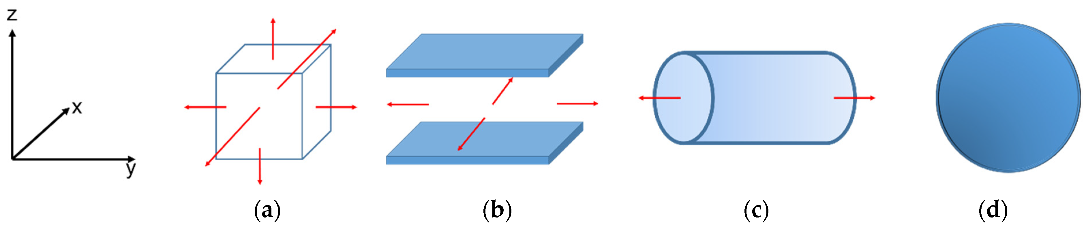
| Infinite slit pore of 5 nm in width | Slit No.1 | Gradual addition of nitrogen molecules in an infinite slit pore having pore length in y-direction of 2 nm. | Group I |
| Slit No.2 | Gradual addition of nitrogen molecules in an infinite slit pore having pore length in y-direction of 20 nm. | Group III | |
| Infinite cylindrical pore of 5 nm in diameter | Cylinder No.1 | Gradual addition of nitrogen molecules in an infinite cylindrical pore having pore length in y-direction of 2 nm. | Group I |
| Cylinder No.2 | Gradual addition of nitrogen molecules in an infinite cylindrical pore having pore length in y-direction of 20 nm. | Group III | |
| Spherical pore of 5 nm in diameter | Sphere | Gradual addition of nitrogen molecules in a spherical pore. | Group I |
| Potential Model of Nitrogen | Interacting Site | x (nm) | y (nm) | z (nm) | σFF (nm) | εFF/kB (K) | q (e) |
|---|---|---|---|---|---|---|---|
| 1-LJ model | N2 | 0 | 0 | 0 | 0.3615 | 101.5 | 0 |
| 2-LJ model | N | −0.055 | 0 | 0 | 0.331 | 36.0 | −0.482 |
| Center site | 0 | 0 | 0 | 0 | 0 | +0.964 | |
| N | +0.055 | 0 | 0 | 0.331 | 36.0 | −0.482 |
| Type of Pore Geometry | Term | Equation |
|---|---|---|
| Spherical pore | where r is the radial distance from pore center and R is pore radius. | |
| Infinite cylindrical pore | where r is the radial distance from pore center and R is pore radius. | |
where F(a,b,c,d) is the hypergeometric function. | ||
| Infinite slit pore | where z is the distance between a particle and the planar surface and H is pore width. | |
Publisher’s Note: MDPI stays neutral with regard to jurisdictional claims in published maps and institutional affiliations. |
© 2022 by the authors. Licensee MDPI, Basel, Switzerland. This article is an open access article distributed under the terms and conditions of the Creative Commons Attribution (CC BY) license (https://creativecommons.org/licenses/by/4.0/).
Share and Cite
Jitmitsumphan, S.; Sripetdee, T.; Chaimueangchuen, T.; Tun, H.M.; Chinkanjanarot, S.; Klomkliang, N.; Srinives, S.; Jonglertjunya, W.; Ling, T.C.; Phadungbut, P. Unveiling the Molecular Origin of Vapor-Liquid Phase Transition of Bulk and Confined Fluids. Molecules 2022, 27, 2656. https://doi.org/10.3390/molecules27092656
Jitmitsumphan S, Sripetdee T, Chaimueangchuen T, Tun HM, Chinkanjanarot S, Klomkliang N, Srinives S, Jonglertjunya W, Ling TC, Phadungbut P. Unveiling the Molecular Origin of Vapor-Liquid Phase Transition of Bulk and Confined Fluids. Molecules. 2022; 27(9):2656. https://doi.org/10.3390/molecules27092656
Chicago/Turabian StyleJitmitsumphan, Sorrasit, Tirayoot Sripetdee, Tharathep Chaimueangchuen, Htet Myet Tun, Sorayot Chinkanjanarot, Nikom Klomkliang, Sira Srinives, Woranart Jonglertjunya, Tau Chuan Ling, and Poomiwat Phadungbut. 2022. "Unveiling the Molecular Origin of Vapor-Liquid Phase Transition of Bulk and Confined Fluids" Molecules 27, no. 9: 2656. https://doi.org/10.3390/molecules27092656
APA StyleJitmitsumphan, S., Sripetdee, T., Chaimueangchuen, T., Tun, H. M., Chinkanjanarot, S., Klomkliang, N., Srinives, S., Jonglertjunya, W., Ling, T. C., & Phadungbut, P. (2022). Unveiling the Molecular Origin of Vapor-Liquid Phase Transition of Bulk and Confined Fluids. Molecules, 27(9), 2656. https://doi.org/10.3390/molecules27092656