
Automated Computational Detection of Disease Activity in ANCA-Associated Glomerulonephritis Using Raman Spectroscopy: A Pilot Study

 ,
, 
Abstract
1. Introduction
2. Materials and Methods
2.1. Patients & Ethics
2.2. Sample Collection & Preparation
2.3. Spectral Acquisition
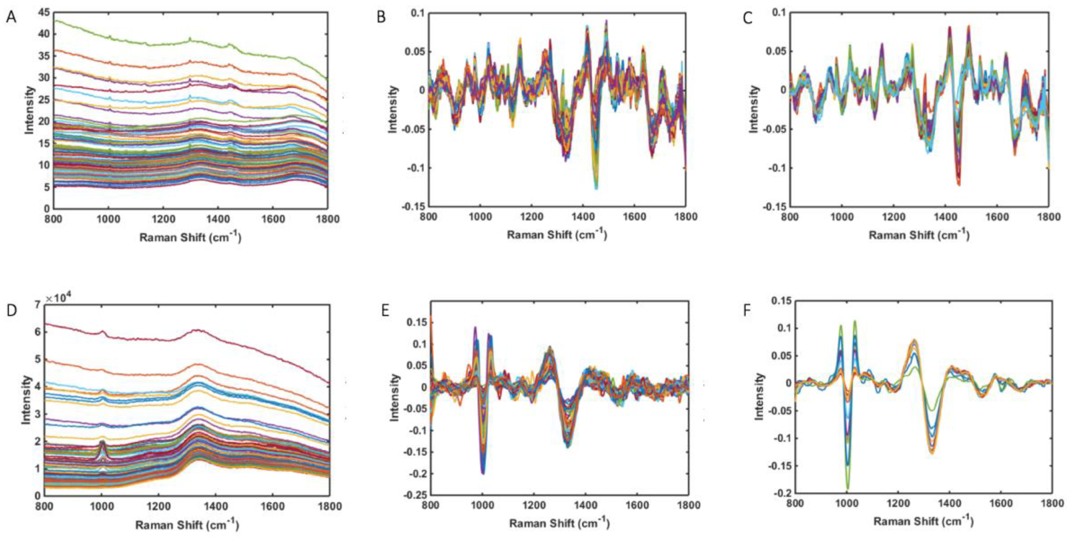
2.4. Spectral Pre-Processing
2.5. Multivariate Analysis
2.6. Chemometric Models
2.7. Model Validation
3. Results
3.1. Study Population
3.2. Spectral Data & Classification Models: All Renal Tissue Samples
3.3. Spectral Data and Classification Models: Comparative Results for Tissue & Paired Urine Samples
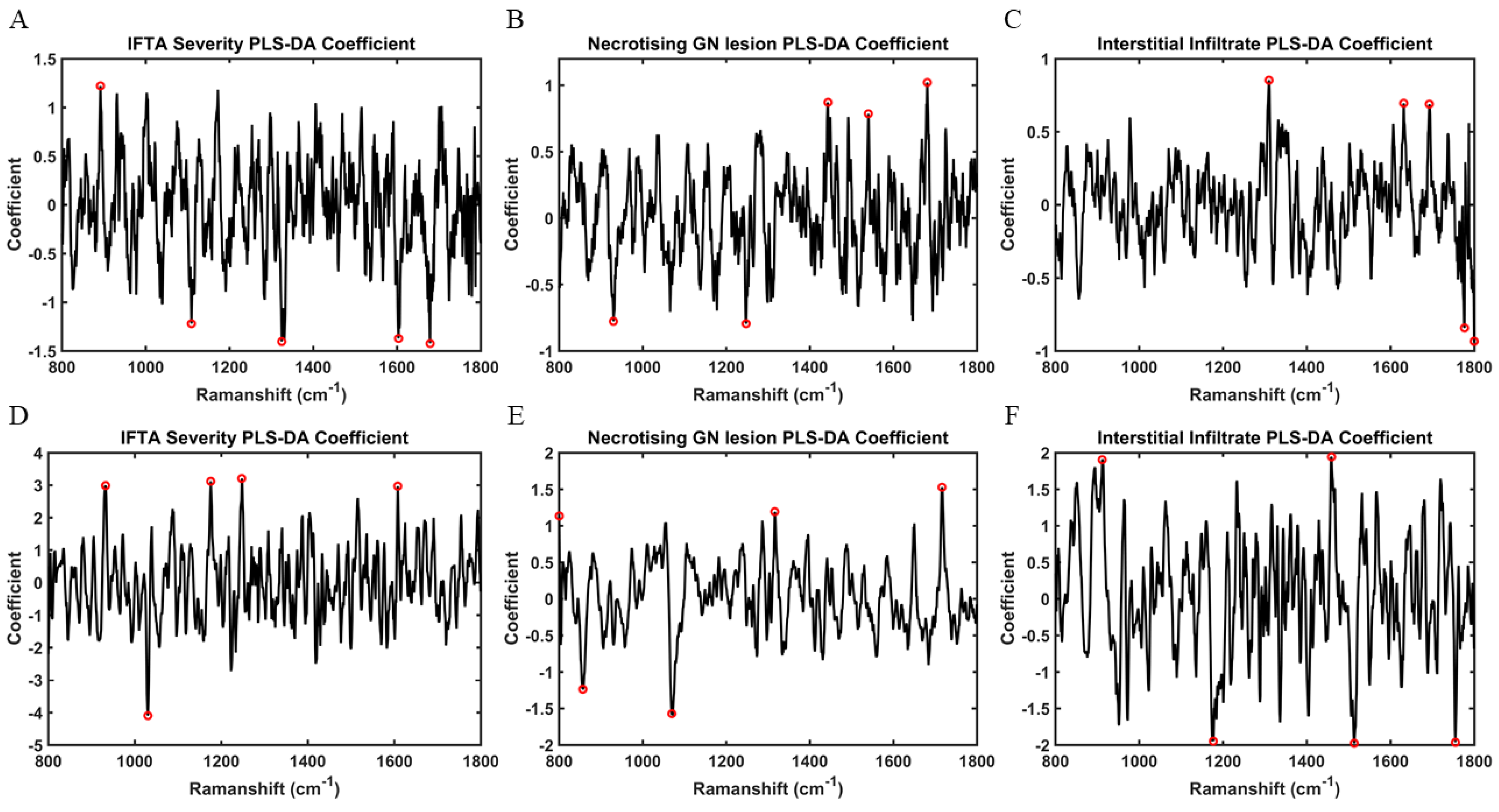
3.4. Key Discriminating Spectral Biomarkers: Tissue & Paired Urine Samples
4. Discussion
Author Contributions
Funding
Institutional Review Board Statement
Informed Consent Statement
Data Availability Statement
Acknowledgments
Conflicts of Interest
References
- Flossmann, O.; Berden, A.; De Groot, K.; Hagen, C.; Harper, L.; Heijl, C.; Höglund, P.; Jayne, D.; Luqmani, R.; Mahr, A.; et al. Long-term patient survival in ANCA-associated vasculitis. Ann. Rheum. Dis. 2011, 70, 488–494. [Google Scholar] [CrossRef]
- de Joode, A.A.E.; Sanders, J.S.F.; Stegeman, C.A. Renal survival in Proteinase 3 and Myeloperoxidase ANCA-associated systemic Vasculitis. Clin. J. Am. Soc. Nephrol. 2013, 8, 1709–1717. [Google Scholar] [CrossRef] [PubMed]
- Berti, A.; Cornec-Le Gall, E.; Cornec, D.; Casal Moura, M.; Matteson, E.L.; Crowson, C.S.; Ravindran, A.; Sethi, S.; Fervenza, F.C.; Specks, U. Incidence, prevalence, mortality and chronic renal damage of anti-neutrophil cytoplasmic antibody-associated glomerulonephritis in a 20-year population-based cohort. Nephrol. Dial. Transplant. 2018, 34, 1508–1517. [Google Scholar] [CrossRef] [PubMed]
- Lee, T.; Gasim, A.; Derebail, V.K.; Chung, Y.; McGregor, J.G.; Lionaki, S.; Poulton, C.; Hogan, S.L.; Jennette, J.C.; Falk, R.J.; et al. Predictors of treatment outcomes in ANCA-associated vasculitis with severe kidney failure. Clin. J. Am. Soc. Nephrol. 2014, 9, 905–913. [Google Scholar] [CrossRef] [PubMed]
- Manno, R.L.; Seo, P.; Geetha, D. Older patients with ANCA-associated vasculitis and dialysis dependent renal failure: A retrospective study. BMC Nephrol. 2015, 16, 88. [Google Scholar] [CrossRef] [PubMed]
- Berden, A.E.; Ferrario, F.; Hagen, E.C.; Jayne, D.R.; Jennette, J.C.; Joh, K.; Neumann, I.; Noël, L.H.; Pusey, C.D.; Waldherr, R.; et al. Histopathologic classification of ANCA-associated glomerulonephritis. J. Am. Soc. Nephrol. 2010, 21, 1628–1636. [Google Scholar] [CrossRef]
- Hilhorst, M.; Wilde, B.; Van Breda Vriesman, P.; Van Paassen, P.; Tervaert, J.W.C. Estimating renal survival using the ANCA-associated GN classification. J. Am. Soc. Nephrol. 2013, 24, 1371–1375. [Google Scholar] [CrossRef]
- Berden, A.E.; Jones, R.B.; Erasmus, D.D.; Walsh, M.; Noël, L.H.; Ferrario, F.; Waldherr, R.; Bruijn, J.A.; Jayne, D.R.; Bajema, I.M. Tubular lesions predict renal outcome in antineutrophil cytoplasmic antibody-associated glomerulonephritis after rituximab therapy. J. Am. Soc. Nephrol. 2012, 23, 313–321. [Google Scholar] [CrossRef]
- Quintana, L.F.; Peréz, N.S.; De Sousa, E.; Rodas, L.M.; Griffiths, M.H.; Solé, M.; Jayne, D. ANCA serotype and histopathological classification for the prediction of renal outcome in ANCA-associated glomerulonephritis. Nephrol. Dial. Transplant. 2014, 29, 1764–1769. [Google Scholar] [CrossRef]
- Chen, Y.X.; Xu, J.; Pan, X.X.; Shen, P.Y.; Li, X.; Ren, H.; Chen, X.N.; Ni, L.Y.; Zhang, W.; Chen, N. Histopathological classification and renal outcome in patients with antineutrophil cytoplasmic antibodies-associated renal vasculitis: A study of 186 patients and meta analysis. J. Rheumatol. 2017, 44, 304–313. [Google Scholar] [CrossRef]
- van Daalen, E.E.; Wester Trejo, M.A.C.; Göçeroglu, A.; Ferrario, F.; Joh, K.; Noël, L.H.; Ogawa, Y.; Wilhelmus, S.; Ball, M.J.; Honsova, E.; et al. Developments in the histopathological classification of ANCA-associated glomerulonephritis. Clin. J. Am. Soc. Nephrol. 2020, 15, 1103–1111. [Google Scholar] [CrossRef] [PubMed]
- Brix, S.R.; Noriega, M.; Tennstedt, P.; Vettorazzi, E.; Busch, M.; Nitschke, M.; Jabs, W.J.; Özcan, F.; Wendt, R.; Hausberg, M.; et al. Development and validation of a renal risk score in ANCA-associated glomerulonephritis. Kidney Int. 2018, 94, 1177–1188. [Google Scholar] [CrossRef] [PubMed]
- Morais, C.L.M.; Lima, K.M.G.; Singh, M.; Martin, F.L. Tutorial: Multivariate classification for vibrational spectroscopy in biological samples. Nat. Protoc. 2020, 15, 2143–2162. [Google Scholar] [CrossRef] [PubMed]
- Morais, C.L.M.; Paraskevaidi, M.; Cui, L.; Fullwood, N.J.; Isabelle, M.; Lima, K.M.G.; Martin-Hirsch, P.L.; Sreedhar, H.; Trevisan, J.; Walsh, M.J.; et al. Standardization of complex biologically derived spectrochemical datasets. Nat. Protoc. 2019, 14, 1546–1577. [Google Scholar] [CrossRef] [PubMed]
- Ballabio, D.; Consonni, V. Classification tools in chemistry. Part 1: Linear models. PLS-DA. Anal. Methods 2013, 5, 3790–3798. [Google Scholar] [CrossRef]
- Cortes, C.; Vapnik, V. Support-Vector Networks. Mach. Learn. 1995, 297, 273–297. [Google Scholar] [CrossRef]
- Morais, C.L.M.; Lima, K. Comparing unfolded and two-dimensional discriminant analysis and support vector machines for classification of EEM data. Chemom. Intell. Lab. Syst. 2017, 162, 123–129. [Google Scholar] [CrossRef]
- Movasaghi, Z.; Rehman, S.; Rehman, I.U. Raman spectroscopy of biological tissues. Appl. Spectrosc. Rev. 2007, 42, 493–541. [Google Scholar] [CrossRef]
- Ginley, B.; Jen, K.-Y.; Han, S.S.; Rodrigues, L.; Jain, S.; Fogo, A.B.; Zuckerman, J.; Walavalkar, V.; Miecznikowski, J.C.; Wen, Y.; et al. Automated Computational Detection of Interstitial Fibrosis, Tubular Atrophy, and Glomerulosclerosis. J. Am. Soc. Nephrol. 2021, 32, 837–850. [Google Scholar] [CrossRef]
- De Bruyne, S.; Van Dorpe, J.; Himpe, J.; Van Biesen, W.; Delanghe, S.; Speeckaert, M.M.; Delanghe, J.R. Detection and Characterization of a Biochemical Signature Associated with Diabetic Nephropathy Using Near-infrared Spectroscopy on Tissue Sections. J. Clin. Med. 2019, 8, 1022. [Google Scholar] [CrossRef]
- Varma, V.K.; Kajdacsy-Balla, A.; Akkina, S.K.; Setty, S.; Walsh, M.J. A label-free approach by infrared spectroscopic imaging for interrogating the biochemistry of diabetic nephropathy progression. Kidney Int. 2016, 89, 1153–1159. [Google Scholar] [CrossRef] [PubMed]
- Severcan, F.; Bozkurt, O.; Gurbanov, R.; Gorgulu, G. FT-IR spectroscopy in diagnosis of diabetes in rat animal model. J. Biophotonics 2010, 3, 621–631. [Google Scholar] [CrossRef] [PubMed]
- Vuiblet, V.; Fere, M.; Gobinet, C.; Birembaut, P.; Piot, O.; Rieu, P. Renal graft fibrosis and inflammation quantification by an automated fourier-transform infrared imaging technique. J. Am. Soc. Nephrol. 2016, 27, 2382–2391. [Google Scholar] [CrossRef]
- Karim, B.; Fleureau, J.; Rolland, D.; Lavastre, O.; Rioux-Leclercq, N.; Guille, F.; Patard, J.-J.; Senhadji, L.; de Crevoisier, R. Raman Spectroscopy: A novel experimental approach to evaluating renal tumours. Eur. Urol. 2010, 58, 602–608. [Google Scholar]
- Couapel, J.-P.; Senhadji, L.; Rioux-Leclercq, N.; Verhoest, G.; Lavastre, O.; de Crevoisier, R.; Al, E. Optical spectroscopy techniques can accurately distinguish benign and malignant renal tumours. BJU Int. 2013, 111, 865–871. [Google Scholar] [CrossRef]
- Mert, S.; Özbek, E.; Ötünçtemur, A.; Çulha, M. Kidney tumor staging using surface-enhanced Raman scattering. J. Biomed. Opt. 2015, 20, 047002. [Google Scholar] [CrossRef]
- Morris, A.D.; Morais, C.L.M.; Lima, K.M.G.; Freitas, D.L.D.; Brady, M.E.; Dhaygude, A.P.; Rowbottom, A.W.; Martin, F.L. Distinguishing active from quiescent disease in ANCA-associated vasculitis using attenuated total reflection Fourier-transform infrared spectroscopy. Sci. Rep. 2021, 11, 9981. [Google Scholar] [CrossRef] [PubMed]
- Morris, A.D.; Morais, C.L.M.; Lima, K.M.G.; Freitas, D.L.D.; Brady, M.E.; Dhaygude, A.P.; Rowbottom, A.W.; Martin, F.L. A comparative analysis of different biofluids using Raman spectroscopy to determine disease activity in ANCA-associated vasculitis. J. Biophotonics 2021, 14, e202000426. [Google Scholar] [CrossRef]
- Tam, F.W.K.; Sanders, J.S.; George, A.; Hammad, T.; Miller, C.; Dougan, T.; Cook, H.T.; Kallenberg, C.G.M.; Gaskin, G.; Levy, J.B.; et al. Urinary monocyte chemoattractant protein-1 (MCP-1) is a marker of active renal vasculitis. Nephrol. Dial. Transplant. 2004, 19, 2761–2768. [Google Scholar] [CrossRef]
- Ohlsson, S.; Bakoush, O.; Tencer, J.; Torffvit, O.; Segelmark, M. Monocyte chemoattractant protein 1 is a prognostic marker in ANCA-associated small vessel vasculitis. Mediat. Inflamm. 2009, 2009, 584916. [Google Scholar] [CrossRef]
- Lieberthal, J.G.; Cuthbertson, D.; Carette, S.; Hoffman, G.S.; Khalidi, N.A.; Koening, C.L.; Langford, C.A.; Maksimowicz-McKinnon, K.; Seo, P.; Specks, U.; et al. Urinary biomarkers in relapsing antineutrophil cytoplasmic antibody-associated vasculitis. J. Rheumatol. 2013, 40, 674–683. [Google Scholar] [CrossRef] [PubMed]
- Jönsson, N.; Erlandsson, E.; Gunnarsson, L.; Pettersson, Å.; Ohlsson, S. Monocyte chemoattractant protein-1 in antineutrophil cytoplasmic autoantibody-associated vasculitis: Biomarker potential and association with polymorphisms in the MCP-1 and the CC chemokine receptor-2 gene. Mediat. Inflamm. 2018, 2018, 6861257. [Google Scholar] [CrossRef] [PubMed]
- O’Reilly, V.P.; Wong, L.; Kennedy, C.; Elliot, L.A.; O’Meachair, S.; Coughlan, A.M.; O’Brien, E.C.; Ryan, M.M.; Sandoval, D.; Connolly, E.; et al. Urinary soluble CD163 in active renal vasculitis. J. Am. Soc. Nephrol. 2016, 27, 2906–2916. [Google Scholar] [CrossRef] [PubMed]
- Xing, G.Q.; Chen, M.; Liu, G.; Heeringa, P.; Zhang, J.J.; Zheng, X.; Jie, E.; Kallenberg, C.G.M.; Zhao, M.H. Complement activation is involved in renal damage in human antineutrophil cytoplasmic autoantibody associated pauci-immune vasculitis. J. Clin. Immunol. 2009, 29, 282–291. [Google Scholar] [CrossRef]
- Hilhorst, M.; Van Paassen, P.; Van Rie, H.; Bijnens, N.; Heerings-Rewinkel, P.; Van Breda Vriesman, P.; Cohen Tervaert, J.W. Complement in ANCA-associated glomerulonephritis. Nephrol. Dial. Transplant. 2015, 32, 1302–1313. [Google Scholar] [CrossRef]
- Gou, S.J.; Yuan, J.; Wang, C.; Zhao, M.H.; Chen, M. Alternative complement pathway activation products in urine and kidneys of patients with ANCA-associated GN. Clin. J. Am. Soc. Nephrol. 2013, 8, 1884–1891. [Google Scholar] [CrossRef]
- Aendekerk, J.P.; Timmermans, S.A.M.E.G.; Busch, M.H.; Potjewijd, J.; Heeringa, P.; Damoiseaux, J.G.M.C.; Reutelingsperger, C.P.; van Paassen, P. Urinary Soluble CD163 and Disease Activity in Biopsy-Proven ANCA-Associated Glomerulonephritis. Clin. J. Am. Soc. Nephrol. 2020, 15, 1740–1748. [Google Scholar] [CrossRef]


| AAGN (n = 27) | |
|---|---|
| Mean Age (SD) | 63 ± 10 |
| Sex | |
| Male Female | 15/27 (55.6%) 12/27 (44.4%) |
| Median serum creatinine at biopsy (μmol/L) | 215 (338–164) |
| Median eGFR at biopsy (mls/min/1.73 m2) | 22 (33–12) |
| ANCA serotype at biopsy | |
| MPO | 12/27 (44.4%) |
| PR3 | 12/27 (44.4%) |
| Negative | 3/27 (11.1%) |
| Mean number of glomeruli per biopsy sample | |
| Berden classification | 20 ± 9 |
| Focal | 15/27 (55.6%) |
| Crescentic | 3/27 (11.1%) |
| Sclerosed | 0 |
| Mixed | 9/27 (33.3%) |
| Normal glomeruli | |
| N0 (>25%) | 21/27 (77.8%) |
| N1 (10–25%) | 2/27 (7.4%) |
| N2 (<10%) | 4/27 (14.8%) |
| IFTA | |
| T0 (≤25%) | 20/27 (74.1%) |
| T1 (>25%) | 7/27 (25.9%) |
| Necrotising glomerular lesions | 16/27 (59.3%) |
| Interstitial infiltrate | 10/27 (37%) |
| Extra-glomerular arteritis | 5/27 (18.5%) |
| Vessel wall necrosis | 4/27 (14.8%) |
| Presence of Histological Features as an Experimental Class | Best Discriminate Model | Spectral Data | Accuracy (%) | Sensitivity (%) | Specificity (%) | F-Score (%) | G-Score (%) |
|---|---|---|---|---|---|---|---|
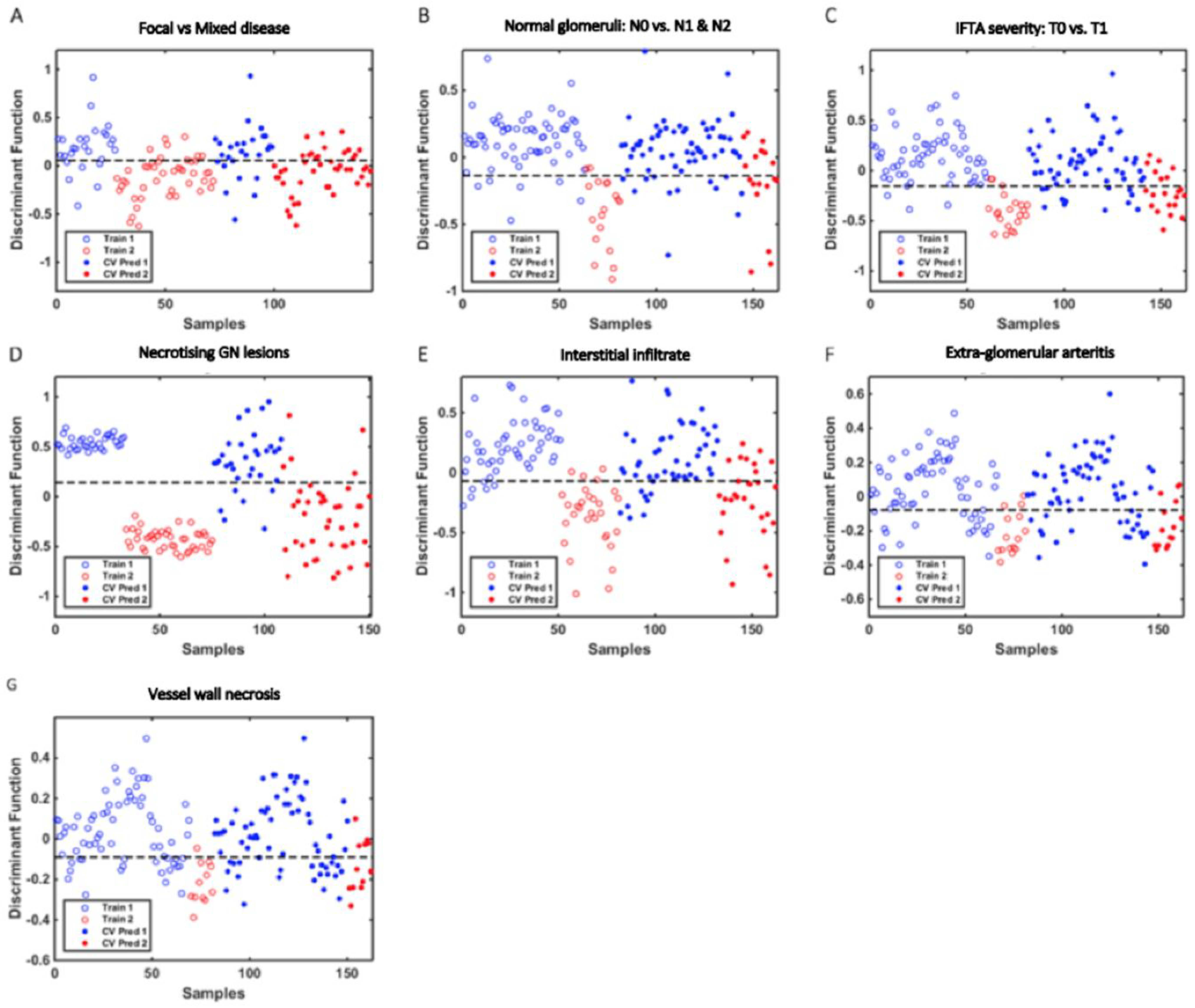
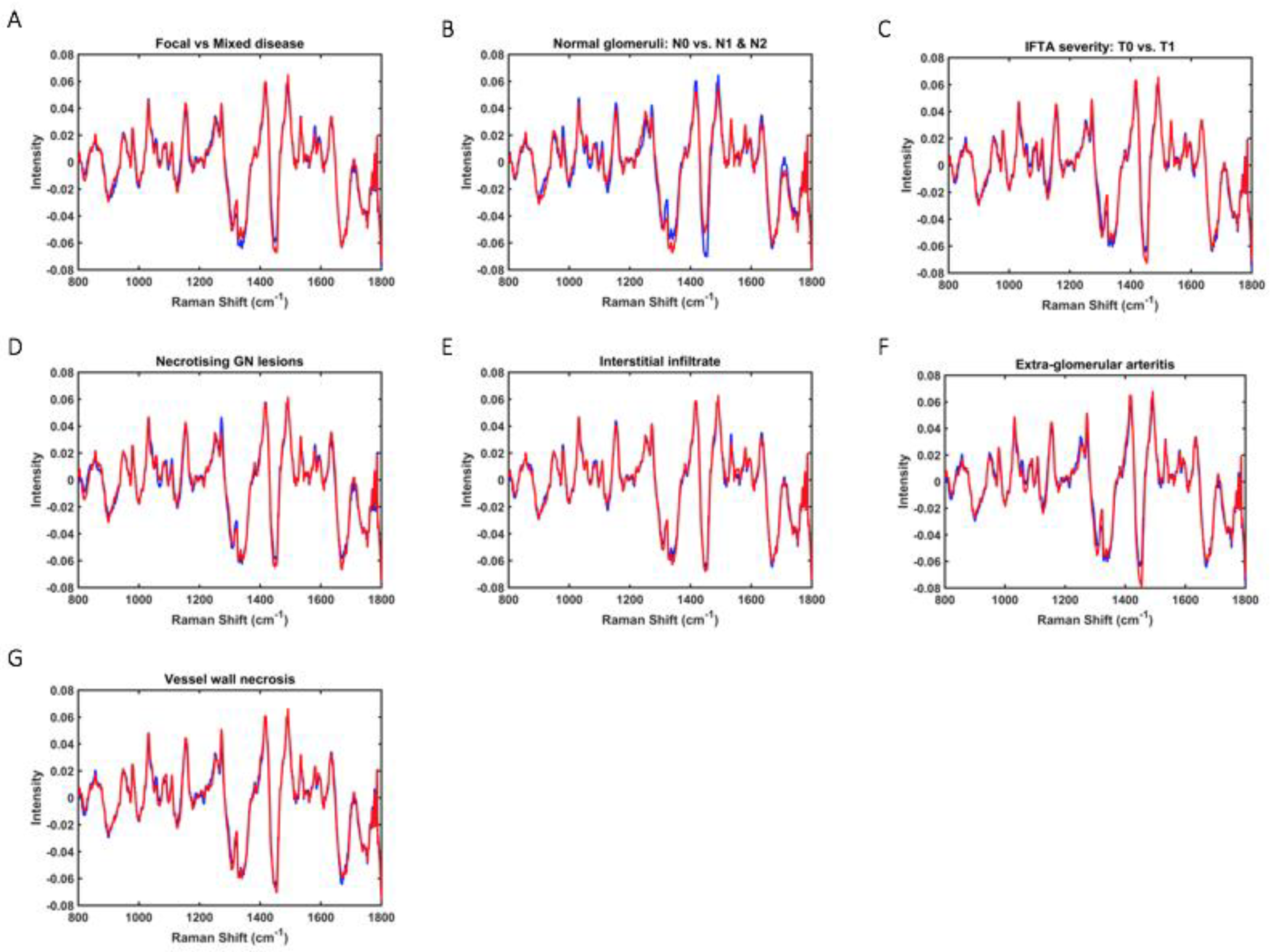
| Berden classification: Focal vs. Mixed | PLS-DA (3 LVs) | Training: TPS | 81 | 82 | 78 | 80 | 80 |
| CV: TPS | 75 | 80 | 67 | 73 | 73 | ||
| Test: MPS | 69 | 69 | 70 | 69 | 69 | ||
| Normal Glomeruli: N0 vs. N1&N2 | PLS-DA (3 LVs) | Training: TPS | 90 | 89 | 90 | 89 | 89 |
| CV: TPS | 77 | 56 | 83 | 67 | 68 | ||
| Test: MPS | 93 | 83 | 95 | 89 | 89 | ||
| IFTA: T0 vs. T1 | PLS-DA (3 LVs) | Training: TPS | 91 | 86 | 93 | 89 | 89 |
| CV: TPS | 78 | 67 | 82 | 74 | 74 | ||
| Test: MPS | 93 | 100 | 90 | 95 | 95 | ||
| Necrotising glomerular lesions | PLS-DA (8 LVs) | Training: TPS | 100 | 100 | 100 | 100 | 100 |
| CV: TPS | 87 | 88 | 85 | 86 | 86 | ||
| Test: MPS | 100 | 100 | 100 | 100 | 100 | ||
| Interstitial Infiltrate | PLS-DA (3 LVs) | Training: TPS | 88 | 87 | 88 | 87 | 87 |
| CV: TPS | 80 | 73 | 84 | 78 | 78 | ||
| Test: MPS | 100 | 100 | 100 | 100 | 100 | ||
| Extra-glomerular arteritis | PLS-DA (2 LVs) | Training: TPS | 74 | 80 | 73 | 76 | 76 |
| CV: TPS | 72 | 67 | 73 | 70 | 70 | ||
| Test: MPS | 78 | 100 | 73 | 84 | 85 | ||
| Vessel Wall Necrosis | PLS-DA (2 LVs) | Training: TPS | 74 | 92 | 71 | 80 | 81 |
| CV: TPS | 69 | 58 | 71 | 64 | 64 | ||
| Test: MPS | 81 | 100 | 78 | 88 | 88 |
| Presence of Histological Features as an Experimental Class | Sample | Best Discriminate Model | Spectral Data | Accuracy (%) | Sensitivity (%) | Specificity (%) | F-Score (%) | G-Score (%) |
|---|---|---|---|---|---|---|---|---|
| Presence of IFTA: T0 vs. T1 | Tissue | PLS-DA (6 LVs) | Training: TPS | 100 | 100 | 100 | 100 | 100 |
| CV: TPS | 83 | 67 | 90 | 77 | 78 | |||
| Test: MPS | 100 | 100 | 100 | 100 | 100 | |||
| Urine | PLS-DA (10 LVs) | Training: TPS | 100 | 100 | 100 | 100 | 100 | |
| CV: TPS | 66 | 57 | 70 | 63 | 63 | |||
| Test: MPS | 100 | 100 | 100 | 100 | 100 | |||
| Presence of Necrotising glomerular lesions | Tissue | PLS-DA (3 LVs) | Training: TPS | 100 | 100 | 100 | 100 | 100 |
| CV: TPS | 87 | 78 | 90 | 84 | 84 | |||
| Test: MPS | 100 | 100 | 100 | 100 | 100 | |||
| Urine | PLS-DA (4 LVs) | Training: TPS | 93 | 93 | 93 | 93 | 93 | |
| CV: TPS | 67 | 53 | 73 | 61 | 62 | |||
| Test: MPS | 100 | 100 | 100 | 100 | 100 | |||
| Presence of Interstitial Infiltrate | Tissue | PLS-DA (6 LVs) | Training: TPS | 100 | 100 | 100 | 100 | 100 |
| CV: TPS | 90 | 89 | 90 | 89 | 89 | |||
| Test: MPS | 100 | 100 | 100 | 100 | 100 | |||
| Urine | PLS-DA (10 LVs) | Training: TPS | 99 | 97 | 100 | 98 | 98 | |
| CV: TPS | 72 | 53 | 80 | 64 | 65 | |||
| Test: MPS | 100 | 100 | 100 | 100 | 100 |
Publisher’s Note: MDPI stays neutral with regard to jurisdictional claims in published maps and institutional affiliations. |
© 2022 by the authors. Licensee MDPI, Basel, Switzerland. This article is an open access article distributed under the terms and conditions of the Creative Commons Attribution (CC BY) license (https://creativecommons.org/licenses/by/4.0/).
Share and Cite
Morris, A.D.; Freitas, D.L.D.; Lima, K.M.G.; Floyd, L.; Brady, M.E.; Dhaygude, A.P.; Rowbottom, A.W.; Martin, F.L. Automated Computational Detection of Disease Activity in ANCA-Associated Glomerulonephritis Using Raman Spectroscopy: A Pilot Study. Molecules 2022, 27, 2312. https://doi.org/10.3390/molecules27072312
Morris AD, Freitas DLD, Lima KMG, Floyd L, Brady ME, Dhaygude AP, Rowbottom AW, Martin FL. Automated Computational Detection of Disease Activity in ANCA-Associated Glomerulonephritis Using Raman Spectroscopy: A Pilot Study. Molecules. 2022; 27(7):2312. https://doi.org/10.3390/molecules27072312
Chicago/Turabian StyleMorris, Adam D., Daniel L. D. Freitas, Kássio M. G. Lima, Lauren Floyd, Mark E. Brady, Ajay P. Dhaygude, Anthony W. Rowbottom, and Francis L. Martin. 2022. "Automated Computational Detection of Disease Activity in ANCA-Associated Glomerulonephritis Using Raman Spectroscopy: A Pilot Study" Molecules 27, no. 7: 2312. https://doi.org/10.3390/molecules27072312
APA StyleMorris, A. D., Freitas, D. L. D., Lima, K. M. G., Floyd, L., Brady, M. E., Dhaygude, A. P., Rowbottom, A. W., & Martin, F. L. (2022). Automated Computational Detection of Disease Activity in ANCA-Associated Glomerulonephritis Using Raman Spectroscopy: A Pilot Study. Molecules, 27(7), 2312. https://doi.org/10.3390/molecules27072312