
Polarisation of Electron Density and Electronic Effects: Revisiting the Carbon–Halogen Bonds

 , , , , , and
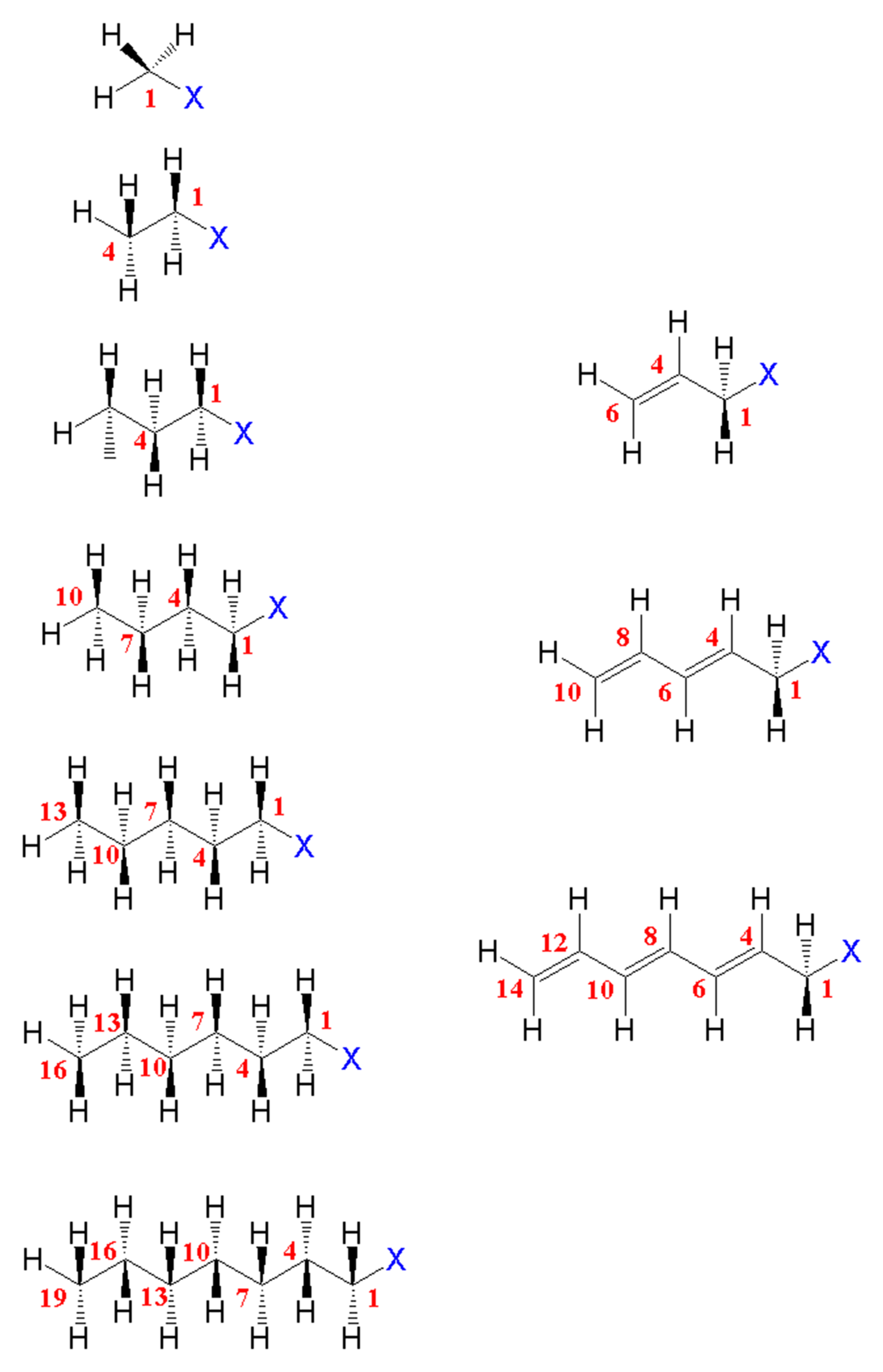
Abstract
:1. Introduction
2. Theoretical Background
3. Materials and Methods
4. Results and Discussion
4.1. Studied Systems
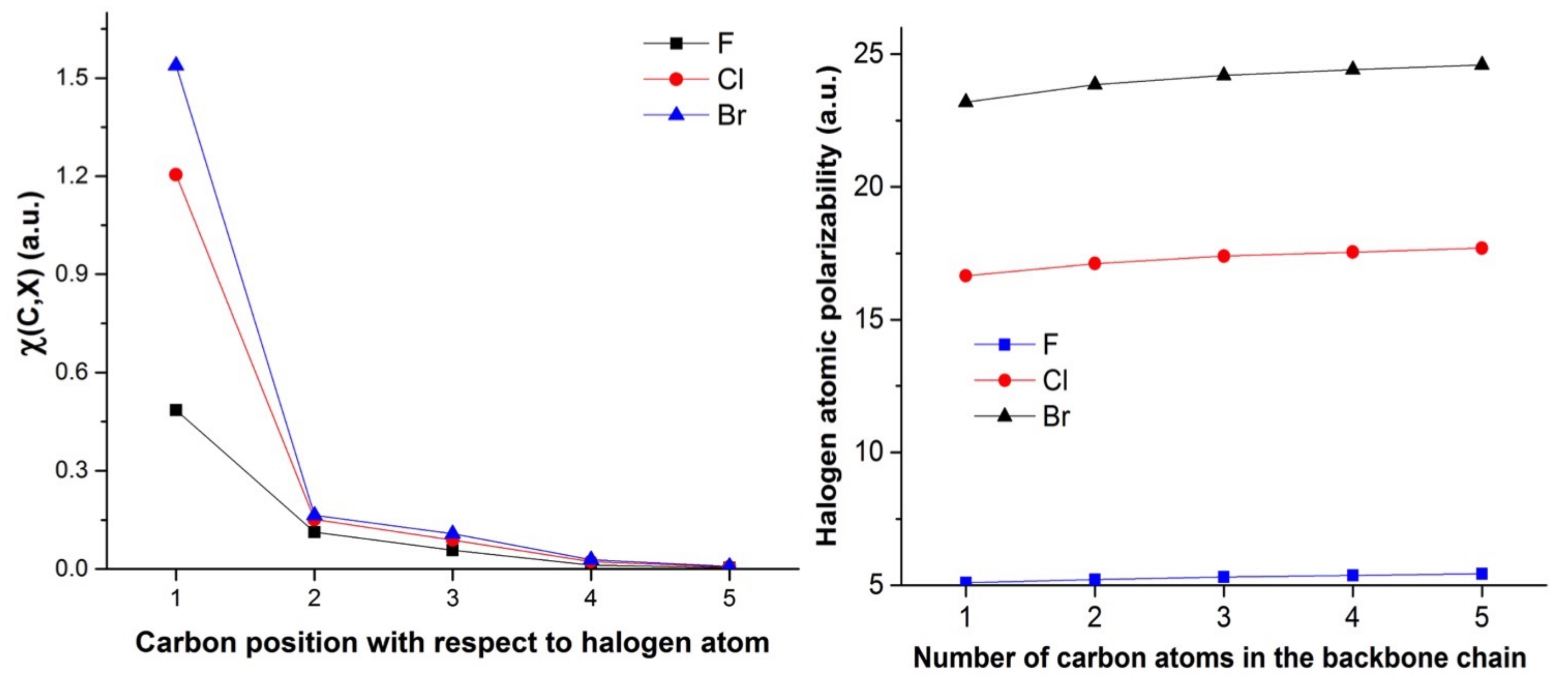
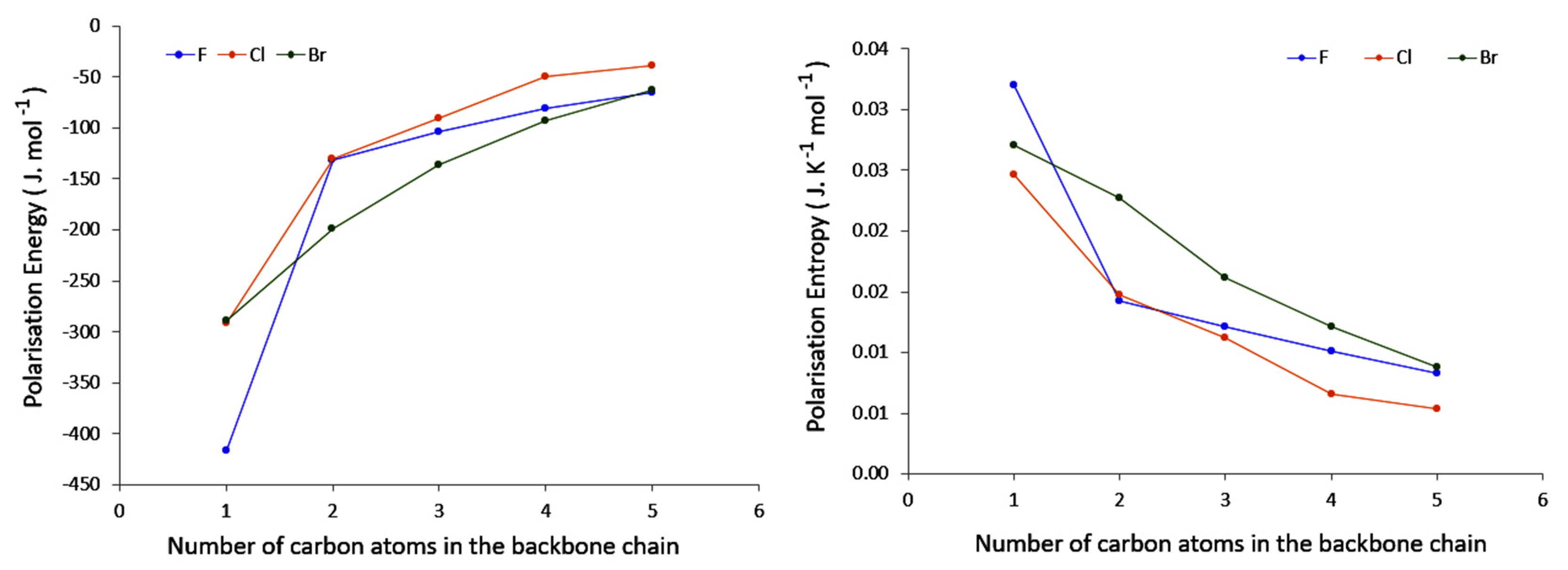
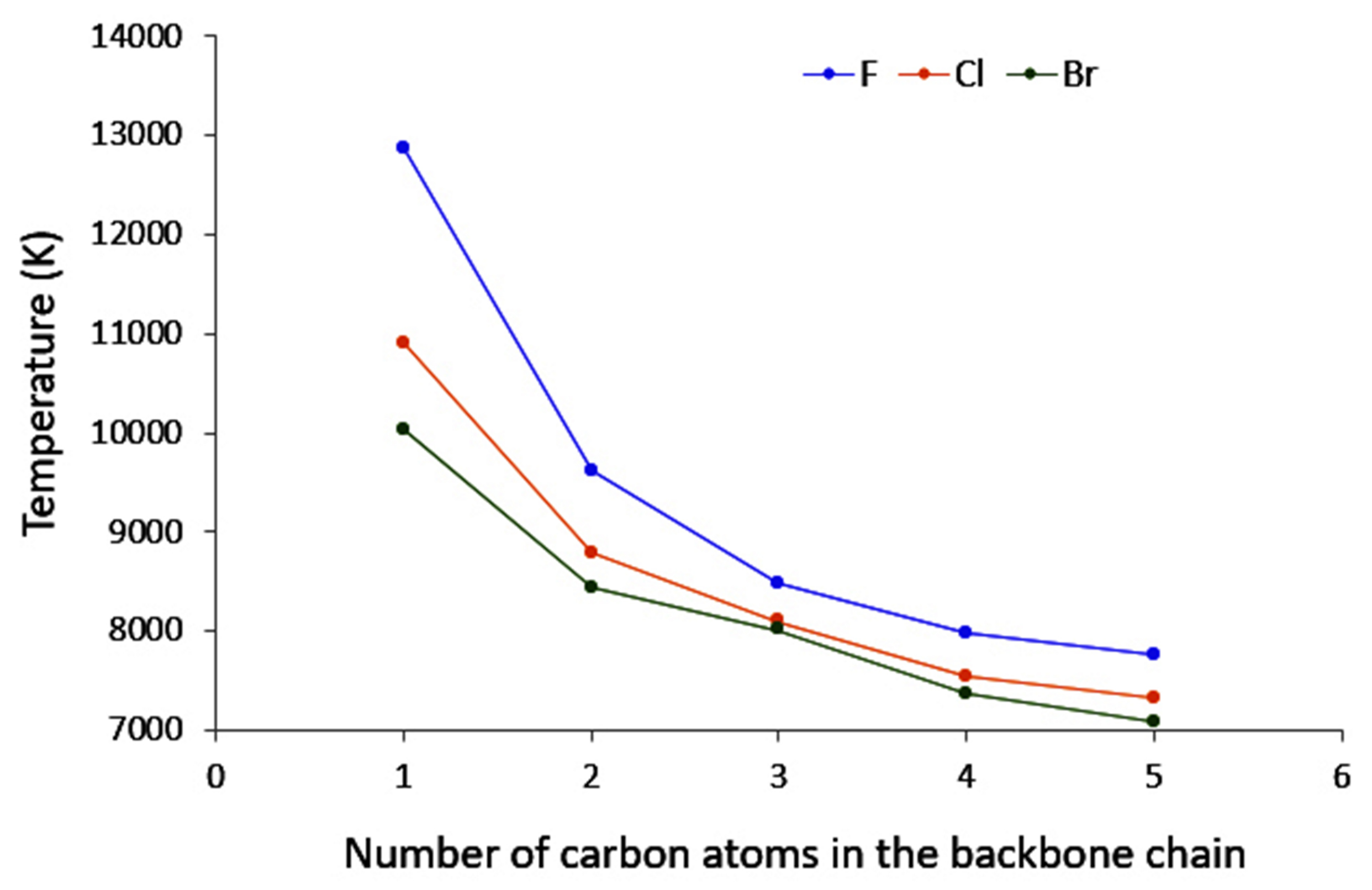
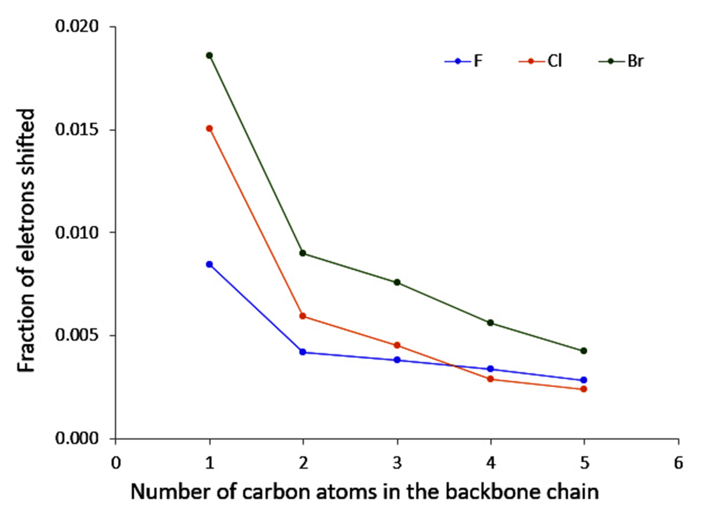
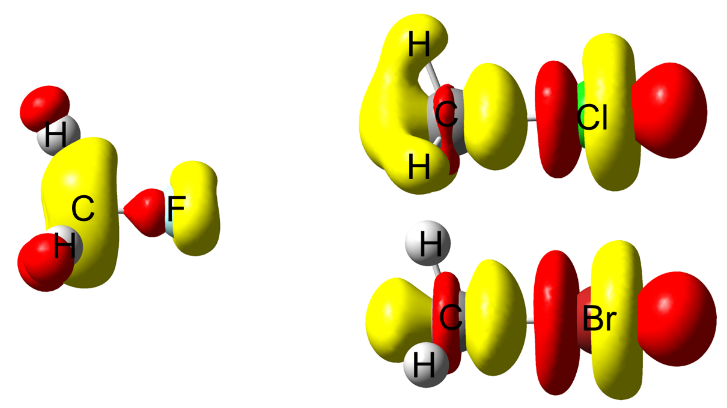
4.2. Saturated Compounds
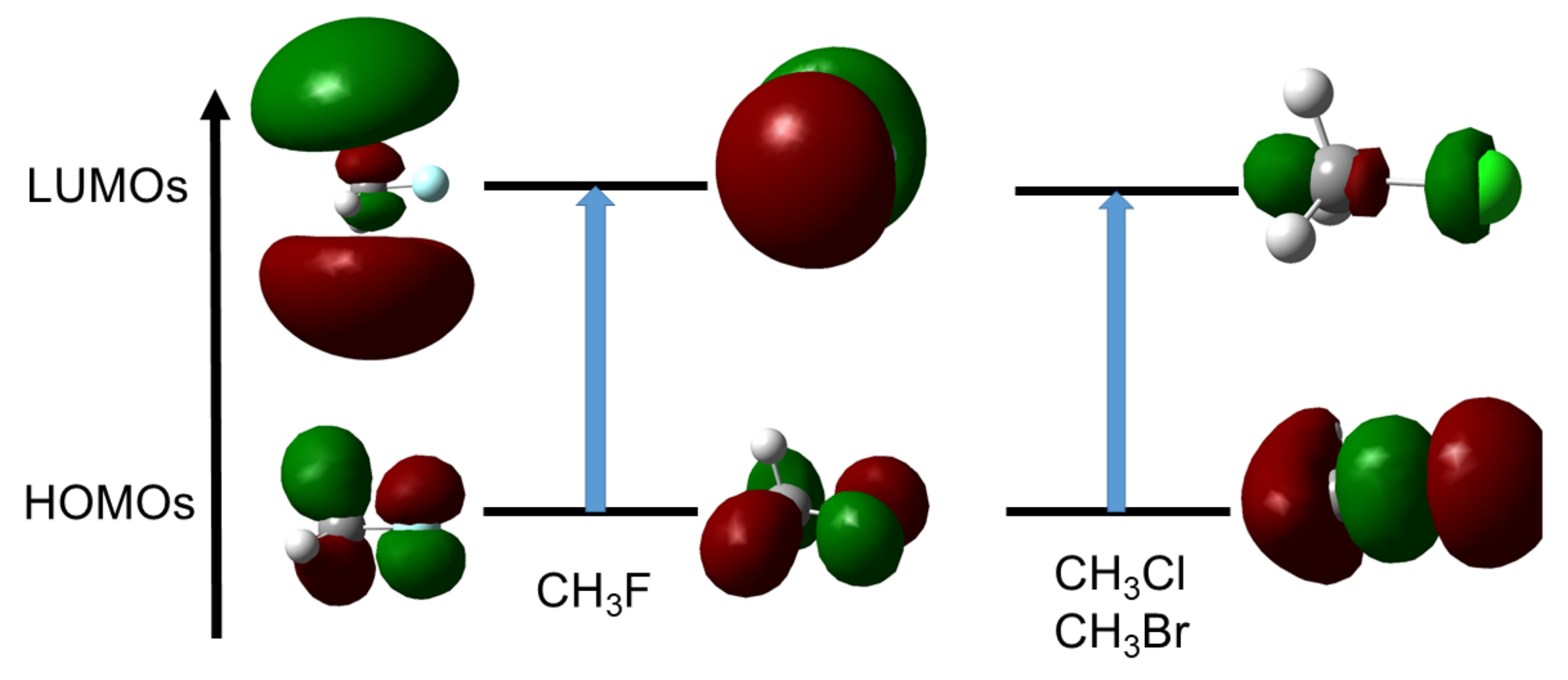
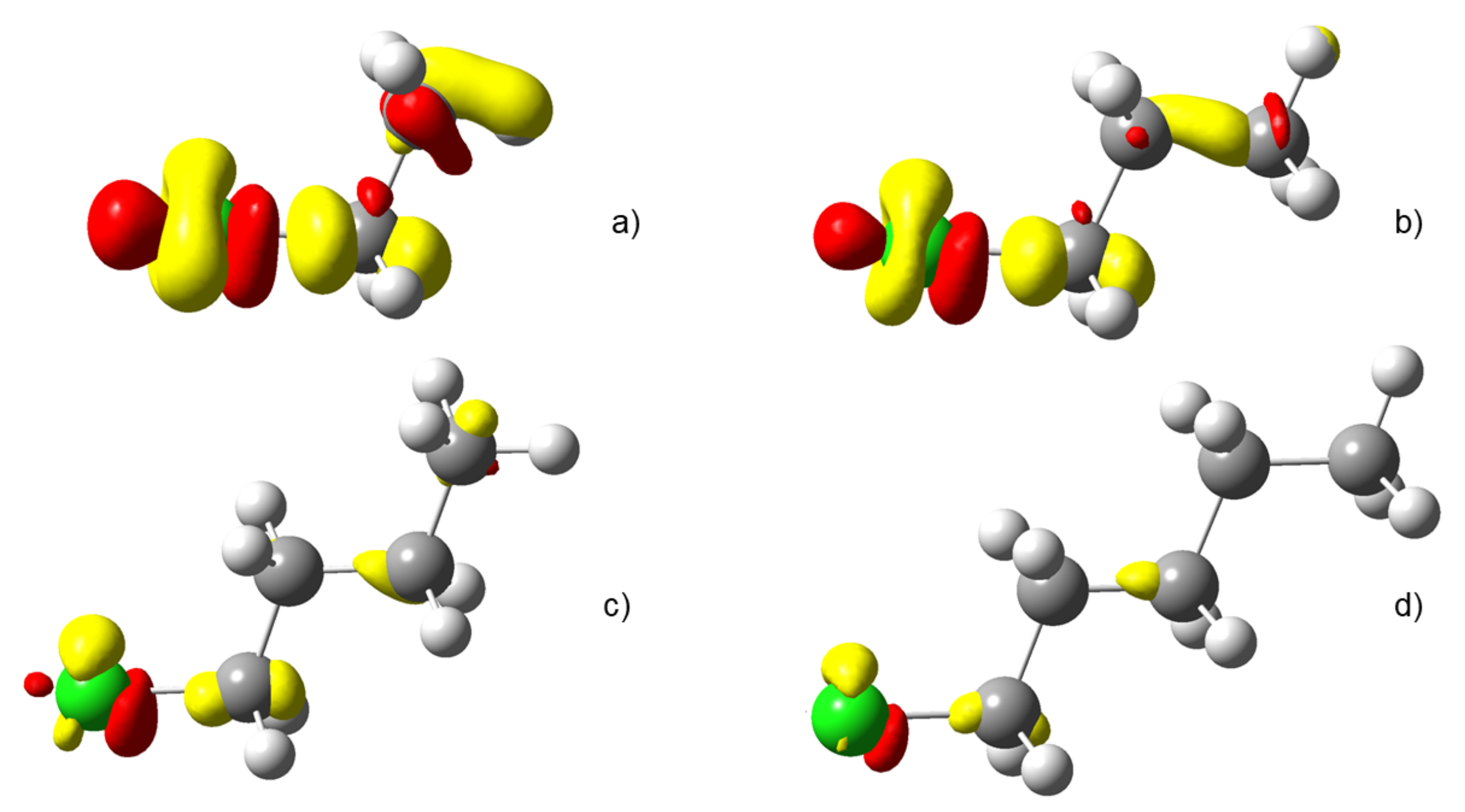
4.3. C-Halides Polarisation Mode
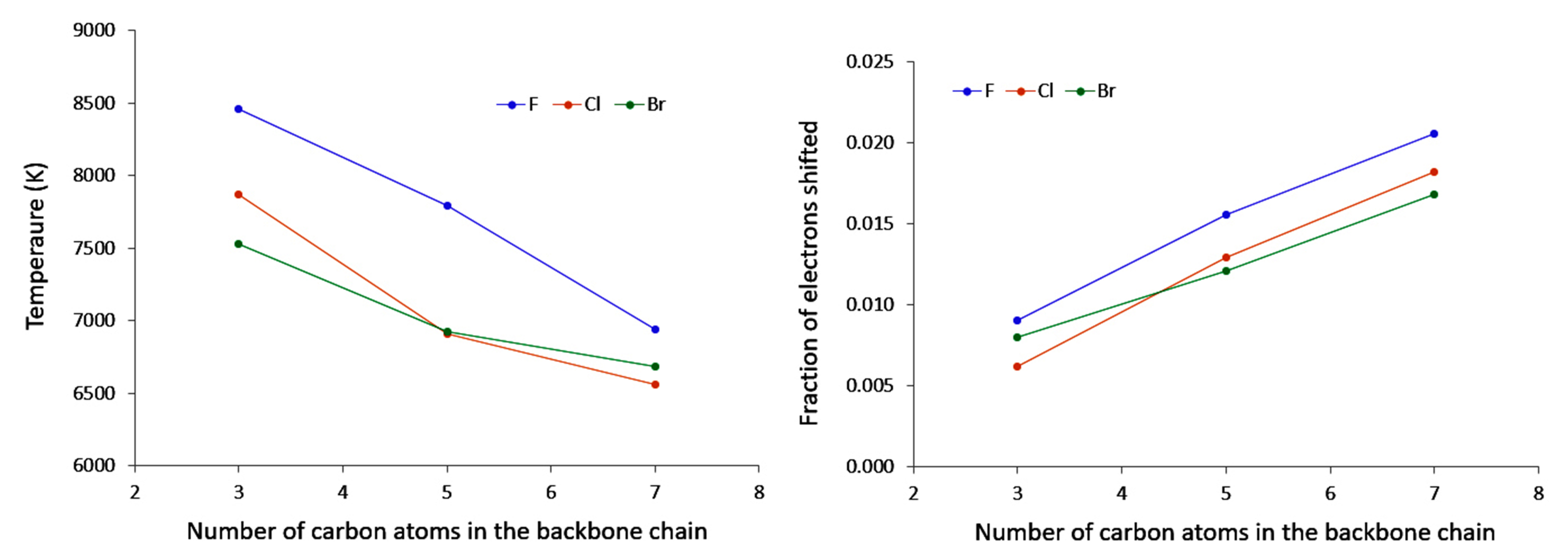
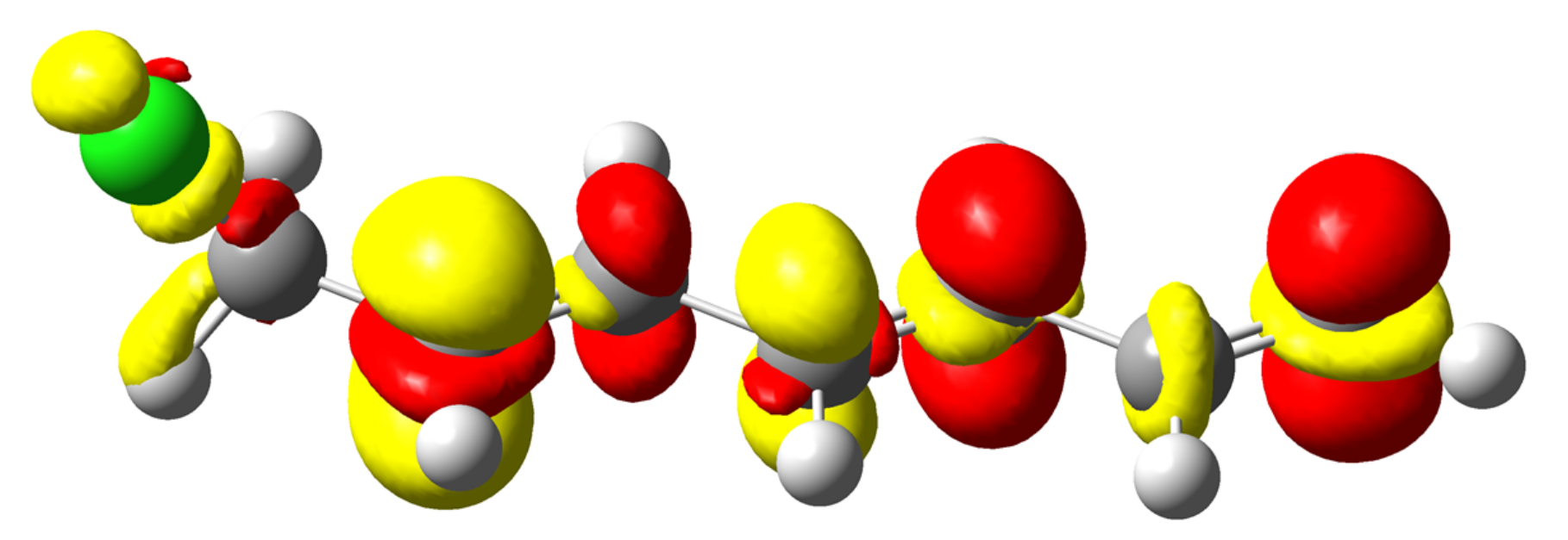
4.4. Unsaturated Compounds
- conjugation, which allows a larger electron density movement, reflecting in the larger values compared to the saturated compounds (and the incident increase in their value with the elongation of the conjugated chain);
- “counter” polarisation of the backbone, stemming from the inductive effects of the halogen, and resulting in a slower decrease of temperature than could be expected.
5. Conclusions
Author Contributions
Funding
Data Availability Statement
Acknowledgments
Conflicts of Interest
Sample Availability
Abbreviations
| AO | atomic orbital |
| C-DFT | Conceptual Density Functional Theory |
| DFT | Density Functional Theory |
| EA | electron affinity |
| EF | electric field |
| IP | ionization potential |
| KS | Kohn–Sham |
| LRF | Linear Response Function |
| MO | molecular orbital |
| NTO | Natural Transition Orbital |
| QTAIM | Quantum Theory of Atoms-in-Molecules |
| RS | Rayleigh–Schrödinger |
| TDA | Tamm–Dancoff Approximation |
References
- Pauling, L. The Nature of the Chemical Bond and the Structure of Molecules and Crystals, 5th ed.; Cornell University Press: Ithaca, NY, USA, 1960. [Google Scholar]
- Shaik, S.; Hiberty, P.C. Valence Bond Theory, Its History, Fundamentals, and Applications: A Primer. In Reviews in Computational Chemistry; John Wiley & Sons, Ltd.: Hoboken, NJ, USA, 2004; Chapter 1; pp. 1–100. [Google Scholar] [CrossRef]
- Mulliken, R.S. A New Electroaffinity Scale; Together with Data on Valence States and on Valence Ionization Potentials and Electron Affinities. J. Chem. Phys. 1934, 2, 782–793. [Google Scholar] [CrossRef]
- Allred, A. Electronegativity values from thermochemical data. J. Inorg. Nucl. Chem. 1961, 17, 215–221. [Google Scholar] [CrossRef]
- Allred, A.; Rochow, E. Electronegativities of carbon, silicon, germanium, tin and lead—II. J. Inorg. Nucl. Chem. 1961, 20, 167–170. [Google Scholar] [CrossRef]
- Gordy, W. A Relation between Bond Force Constants, Bond Orders, Bond Lengths, and the Electronegativities of the Bonded Atoms. J. Chem. Phys. 1946, 14, 305–320. [Google Scholar] [CrossRef]
- Pritchard, H.O. The Determination of Electron Affinities. Chem. Rev. 1953, 52, 529–563. [Google Scholar] [CrossRef]
- Tognetti, V.; Morell, C.; Joubert, L. Atomic electronegativities in molecules. Chem. Phys. Lett. 2015, 635, 111–115. [Google Scholar] [CrossRef]
- Tantardini, C.; Oganov, A.R. Thermochemical electronegativities of the elements. Nat. Commun. 2021, 12. [Google Scholar] [CrossRef]
- Chermette, H. An old, but actual concept: The electronegativity, and its connection to HSAB principle. l’Actualité Chimique 1985, 120, 59–69. (In French) [Google Scholar]
- Parr, R.G.; Donnelly, R.A.; Levy, M.; Palke, W.E. Electronegativity: The density functional viewpoint. J. Chem. Phys. 1978, 68, 3801–3807. [Google Scholar] [CrossRef]
- Chermette, H. Chemical reactivity indexes in density functional theory. J. Comput. Chem. 1999, 20, 129–154. [Google Scholar] [CrossRef]
- Geerlings, P.; De Proft, F.; Langenaeker, W. Conceptual Density Functional Theory. Chem. Rev. 2003, 103, 1793–1874. [Google Scholar] [CrossRef]
- Blanksby, S.J.; Ellison, G.B. Bond Dissociation Energies of Organic Molecules. Accounts Chem. Res. 2003, 36, 255–263. [Google Scholar] [CrossRef]
- Geerlings, P.; Chamorro, E.; Chattaraj, P.K.; De Proft, F.; Gazquez, J.L.; Liu, S.; Morell, C.; Toro-Labbe, A.; Vela, A.; Ayers, P. Conceptual density functional theory: Status, prospects, issues. Theor. Chem. Accounts 2020, 139, 36. [Google Scholar] [CrossRef]
- Geerlings, P.; De Proft, F. Recent developments in conceptual density functional theory. In Abstracts of Papers of the American Chemical Society, Proceedings of the 231st National Meeting of the American-Chemical-Society, Atlanta, GA, USA, 26–30 March 2006; American Chemical Society: Washington, DC, USA, 2006; Volume 231, p. 231. [Google Scholar]
- Sablon, N.; Proft, F.D.; Geerlings, P. The linear response kernel of conceptual DFT as a measure of electron delocalisation. Chem. Phys. Lett. 2010, 498, 192–197. [Google Scholar] [CrossRef]
- Boisdenghien, Z.; Van Alsenoy, C.; De Proft, F.; Geerlings, P. Evaluating and Interpreting the Chemical Relevance of the Linear Response Kernel for Atoms. J. Chem. Theory Comput. 2013, 9, 1007–1015. [Google Scholar] [CrossRef]
- Boisdenghien, Z.; Fias, S.; Pieve, F.D.; Proft, F.D.; Geerlings, P. The polarisability of atoms and molecules: A comparison between a conceptual density functional theory approach and time-dependent density functional theory. Mol. Phys. 2015, 113, 1890–1898. [Google Scholar] [CrossRef]
- Guégan, F.; Tognetti, V.; Martínez-Araya, J.I.; Chermette, H.; Merzoud, L.; Toro-Labbé, A.; Morell, C. A statistical thermodynamics view of electron density polarisation: Application to chemical selectivity. Phys. Chem. Chem. Phys. 2020, 22, 23553–23562. [Google Scholar] [CrossRef]
- Berkowitz, M.; Parr, R.G. Molecular hardness and softness, local hardness and softness, hardness and softness kernels, and relations among these quantities. J. Chem. Phys. 1988, 88, 2554–2557. [Google Scholar] [CrossRef]
- Scherrer, A.; Sebastiani, D. Moment expansion of the linear density-density response function. J. Comput. Chem. 2016, 37, 665–674. [Google Scholar] [CrossRef]
- Senet, P. Variational Principle for Eigenmodes of Reactivity in Conceptual Density Functional Theory. ACS Omega 2020, 5, 25349–25357. [Google Scholar] [CrossRef]
- Guégan, F.; Pigeon, T.; De Proft, F.; Tognetti, V.; Joubert, L.; Chermette, H.; Ayers, P.W.; Luneau, D.; Morell, C. Understanding Chemical Selectivity through Well Selected Excited States. J. Phys. Chem. A 2020, 124, 633–641. [Google Scholar] [CrossRef] [Green Version]
- Neese, F. The ORCA program system. WIREs Comput. Mol. Sci. 2012, 2, 73–78. [Google Scholar] [CrossRef]
- Hirata, S.; Head-Gordon, M. Time-dependent density functional theory within the Tamm-Dancoff approximation. Chem. Phys. Lett. 1999, 314, 291–299. [Google Scholar] [CrossRef]
- Geerlings, P.; Fias, S.; Boisdenghien, Z.; De Proft, F. Conceptual DFT: Chemistry from the linear response function. Chem. Soc. Rev. 2014, 43, 4989–5008. [Google Scholar] [CrossRef]
- Bader, R.F.W. Atoms in Molecules: A Quantum Theory; Clarendon: Owxford, UK, 1990. [Google Scholar]
- te Velde, G.; Bickelhaupt, F.M.; Baerends, E.J.; Fonseca Guerra, C.; van Gisbergen, S.J.A.; Snijders, J.G.; Ziegler, T. Chemistry with ADF. J. Comput. Chem. 2001, 22, 931–967. [Google Scholar] [CrossRef]
- Baerends, E.J.; Ziegler, T.; Atkins, A.J.; Autschbach, J.; Baseggio, O.; Bashford, D.; Bérces, A.; Bickelhaupt, F.M.; Bo, C.; Boerritger, P.M.; et al. ADF2021, SCM, Theoretical Chemistry; Vrije Universiteit: Amsterdam, The Netherlands, 2021. [Google Scholar]
- Dos Santos, L.H.R.; Krawczuk, A.; Macchi, P. Distributed Atomic Polarizabilities of Amino Acids and their Hydrogen-Bonded Aggregates. J. Phys. Chem. A 2015, 119, 3285–3298. [Google Scholar] [CrossRef]
- Frisch, M.J.; Trucks, G.W.; Schlegel, H.B.; Scuseria, G.E.; Robb, M.A.; Cheeseman, J.R.; Scalmani, G.; Barone, V.; Petersson, G.A.; Nakatsuji, H.; et al. Gaussian 09 Revision C.01; Gaussian Inc.: Wallingford, CT, USA, 2013. [Google Scholar]
- Keith, T.A. AIMAll (Version 19.02.13); TK Gristmill Software: Overland Park, KS, USA, 2019. [Google Scholar]
- Dumont, E.; Chaquin, P. Investigation of pure inductive effects on benzene ring by 13C NMR chemical shifts: A theoretical study using fictitious nuclear charges of hydrogen atoms (’H* method’). Chem. Phys. Lett. 2007, 435, 354–357. [Google Scholar] [CrossRef]


Publisher’s Note: MDPI stays neutral with regard to jurisdictional claims in published maps and institutional affiliations. |
© 2021 by the authors. Licensee MDPI, Basel, Switzerland. This article is an open access article distributed under the terms and conditions of the Creative Commons Attribution (CC BY) license (https://creativecommons.org/licenses/by/4.0/).
Share and Cite
Menant, S.; Guégan, F.; Tognetti, V.; Merzoud, L.; Joubert, L.; Chermette, H.; Morell, C. Polarisation of Electron Density and Electronic Effects: Revisiting the Carbon–Halogen Bonds. Molecules 2021, 26, 6218. https://doi.org/10.3390/molecules26206218
Menant S, Guégan F, Tognetti V, Merzoud L, Joubert L, Chermette H, Morell C. Polarisation of Electron Density and Electronic Effects: Revisiting the Carbon–Halogen Bonds. Molecules. 2021; 26(20):6218. https://doi.org/10.3390/molecules26206218
Chicago/Turabian StyleMenant, Sébastien, Frédéric Guégan, Vincent Tognetti, Lynda Merzoud, Laurent Joubert, Henry Chermette, and Christophe Morell. 2021. "Polarisation of Electron Density and Electronic Effects: Revisiting the Carbon–Halogen Bonds" Molecules 26, no. 20: 6218. https://doi.org/10.3390/molecules26206218
APA StyleMenant, S., Guégan, F., Tognetti, V., Merzoud, L., Joubert, L., Chermette, H., & Morell, C. (2021). Polarisation of Electron Density and Electronic Effects: Revisiting the Carbon–Halogen Bonds. Molecules, 26(20), 6218. https://doi.org/10.3390/molecules26206218