Appendix A
The appendix includes informational materials that show the featurization of the GNN and non-GNN baseline models in
Table A7, in
Figure A1 and
Figure A2 the individual models and their corresponding names can be seen. These are the same Figures as in the main body but include the unique identifiers. These identifiers show what kind of model type, featurization and training approach was used when looked up in
Table A8,
Table A9,
Table A10,
Table A11,
Table A12,
Table A13,
Table A14,
Table A15,
Table A16,
Table A17,
Table A18 and
Table A19. The run-time to fit the used RF, SVM, and KNN models with 3380 compounds on logD is approximately 50 s (RF), 25 s (SVM), and 0.5 s (KNN). When training the GNN model types on the 3380 logD compounds it takes for each epoch approximately 56 s (D-GIN), 35 s (D-MPNN), and 28 s (GIN).
Table A1.
Node and edge featurization of type 3. Each node or edge featurization vector consisted of a concatenation of the different one-hot encoded or floating point feature vectors according to their possible states (if present) and corresponding size-36 for nodes and 20 for edges.
Table A1.
Node and edge featurization of type 3. Each node or edge featurization vector consisted of a concatenation of the different one-hot encoded or floating point feature vectors according to their possible states (if present) and corresponding size-36 for nodes and 20 for edges.
| Feature | Possible States | Size |
|---|
| chemical element | H, C, N, O, S, F, P, Cl, Br, I | 10 |
| calculated formal charge | −2, −1, 0, 1, 2 | 5 |
| CIP configuration | R, S, None, either | 4 |
| hybridization state | sp, sp2, sp3, sp3d, sp3d2, none | 6 |
| amide center | yes, no | 2 |
| present in aromatic ring | yes, no | 2 |
| ring size | 1/size | 1 |
| nr. of hydrogens | 0, 1, 2, 3, 4, 5 | 6 |
| bond order | 1, 2, 3 | 3 |
| conjugated | yes, no | 2 |
| rotate−able | yes, no | 2 |
| amide bond | yes, no | 2 |
| present in aromatic ring | yes, no | 2 |
| present in ring | yes, no | 2 |
| ring size | 1/size | 1 |
| CIP configuration | none, E, Z, trans, cis, either | 6 |
Table A2.
Node and edge featurization of type 4. Each node or edge featurization vector consisted of a concatenation of the different one-hot encoded or floating point feature vectors according to their possible states (if present) and corresponding size-45 for nodes and 29 for edges.
Table A2.
Node and edge featurization of type 4. Each node or edge featurization vector consisted of a concatenation of the different one-hot encoded or floating point feature vectors according to their possible states (if present) and corresponding size-45 for nodes and 29 for edges.
| Feature | Possible States | Size |
|---|
| chemical element | H, C, N, O, S, F, P, Cl, Br, I | 10 |
| calculated formal charge | −2, −1, 0, 1, 2 | 5 |
| CIP configuration | R, S, None, either | 4 |
| hybridization state | sp, sp2, sp3, sp3d, sp3d2, none | 6 |
| amide center | yes, no | 2 |
| present in aromatic ring | yes, no | 2 |
| ring size | 0, 3, 4, 5, 6, 7, 8, 9, 10, 11 | 1 |
| nr. of hydrogens | 0, 1, 2, 3, 4, 5 | 6 |
| bond order | 1, 2, 3 | 3 |
| conjugated | yes, no | 2 |
| rotate-able | yes, no | 2 |
| amide bond | yes, no | 2 |
| present in aromatic ring | yes, no | 2 |
| present in ring | yes, no | 2 |
| ring size | 0, 3, 4, 5, 6, 7, 8, 9, 10, 11 | 1 |
| CIP configuration | none, E, Z, trans, cis, either | 6 |
Table A3.
Node and edge featurization of type 5. Each node or edge featurization vector consisted of a concatenation of the different one-hot encoded or floating point feature vectors according to their possible states (if present) and corresponding size-15 for nodes and 3 for edges.
Table A3.
Node and edge featurization of type 5. Each node or edge featurization vector consisted of a concatenation of the different one-hot encoded or floating point feature vectors according to their possible states (if present) and corresponding size-15 for nodes and 3 for edges.
| Feature | Possible States | Size |
|---|
| chemical element | H, C, N, O, S, F, P, Cl, Br, I | 10 |
| calculated formal charge | −2, −1, 0, 1, 2 | 5 |
| CIP configuration | - | - |
| hybridization state | - | - |
| amide center | - | - |
| present in aromatic ring | - | - |
| ring size | - | - |
| nr. of hydrogens | - | - |
| bond order | 1, 2, 3 | 3 |
| conjugated | - | - |
| rotate-able | - | - |
| amide bond | - | - |
| present in aromatic ring | - | - |
| present in ring | - | - |
| ring size | - | - |
| CIP configuration | - | - |
Table A4.
Node and edge featurization of type 6. Each node or edge featurization vector consisted of a concatenation of the different one-hot encoded or floating point feature vectors according to their possible states (if present) and corresponding size-15 for nodes and 20 for edges.
Table A4.
Node and edge featurization of type 6. Each node or edge featurization vector consisted of a concatenation of the different one-hot encoded or floating point feature vectors according to their possible states (if present) and corresponding size-15 for nodes and 20 for edges.
| Feature | Possible States | Size |
|---|
| chemical element | H, C, N, O, S, F, P, Cl, Br, I | 10 |
| calculated formal charge | −2, −1, 0, 1, 2 | 5 |
| CIP configuration | - | - |
| hybridization state | - | - |
| amide center | - | - |
| present in aromatic ring | - | - |
| present in ring | - | - |
| nr. of hydrogens | - | - |
| bond order | 1, 2, 3 | 3 |
| conjugated | yes, no | 2 |
| rotate-able | yes, no | 2 |
| amide bond | yes, no | 2 |
| present in aromatic ring | yes, no | 2 |
| present in ring | yes, no | 2 |
| ring size | 1/size | 1 |
| CIP configuration | none, E, Z, trans, cis, either | 6 |
Table A5.
Node and edge featurization of type 7. Each node or edge featurization vector consisted of a concatenation of the different one-hot encoded or floating point feature vectors according to their possible states (if present) and corresponding size-36 for nodes and 3 for edges.
Table A5.
Node and edge featurization of type 7. Each node or edge featurization vector consisted of a concatenation of the different one-hot encoded or floating point feature vectors according to their possible states (if present) and corresponding size-36 for nodes and 3 for edges.
| Feature | Possible States | Size |
|---|
| chemical element | H, C, N, O, S, F, P, Cl, Br, I | 10 |
| calculated formal charge | −2, −1, 0, 1, 2 | 5 |
| CIP configuration | R, S, None, either | 4 |
| hybridization state | sp, sp2, sp3, sp3d, sp3d2, none | 6 |
| amide center | yes, no | 2 |
| present in aromatic ring | yes, no | 2 |
| ring size | 0, 3, 4, 5, 6, 7, 8, 9, 10, 11 | 1 |
| nr. of hydrogens | 0, 1, 2, 3, 4, 5 | 6 |
| bond order | 1, 2, 3 | 3 |
| conjugated | - | - |
| rotate-able | - | - |
| amide bond | - | - |
| present in aromatic ring | - | - |
| present in ring | - | - |
| ring size | - | - |
| CIP configuration | - | - |
Table A6.
Node and edge featurization of type 8. Each node or edge featurization vector consisted of a concatenation of the different one-hot encoded or floating point feature vectors according to their possible states (if present) and corresponding size-26 for nodes and 7 for edges.
Table A6.
Node and edge featurization of type 8. Each node or edge featurization vector consisted of a concatenation of the different one-hot encoded or floating point feature vectors according to their possible states (if present) and corresponding size-26 for nodes and 7 for edges.
| Feature | Possible States | Size |
|---|
| chemical element | H, C, N, O, S, F, P, Cl, Br, I | 10 |
| formal charge | −2, −1, 0, 1, 2 | 5 |
| CIP priority rule | R, S, None, either | 4 |
| hybridization state | sp, sp2, sp3, sp3d, sp3d2, none | 6 |
| amide center | - | - |
| aromaticity | - | - |
| ring size | float (1/size) | 1 |
| nr. of hydrogens | - | - |
| bond order | 1, 2, 3 | 3 |
| conjugated | - | - |
| rotate-able | yes, no | 2 |
| amide bond | - | - |
| aromaticity | - | - |
| present in ring | yes, no | 2 |
| ring size | - | - |
| CIP priority rule | - | - |
Table A7.
Non-GNN featurization. The identifier is used as reference.
Table A7.
Non-GNN featurization. The identifier is used as reference.
| Identifier | Fingerprint | Radius | nr. Bits | Descriptor |
|---|
| 10 | ECFP | 4 | 1024 | No |
| 11 | ECFP | 4 | 1536 | No |
| 12 | ECFP | 4 | 2048 | No |
| 13 | MACCSKeys | - | - | No |
| 14 | ECFP | 4 | 1024 | Yes |
| 15 | ECFP | 4 | 1536 | Yes |
| 16 | ECFP | 4 | 2048 | Yes |
| 17 | MACCSKeys | - | - | Yes |
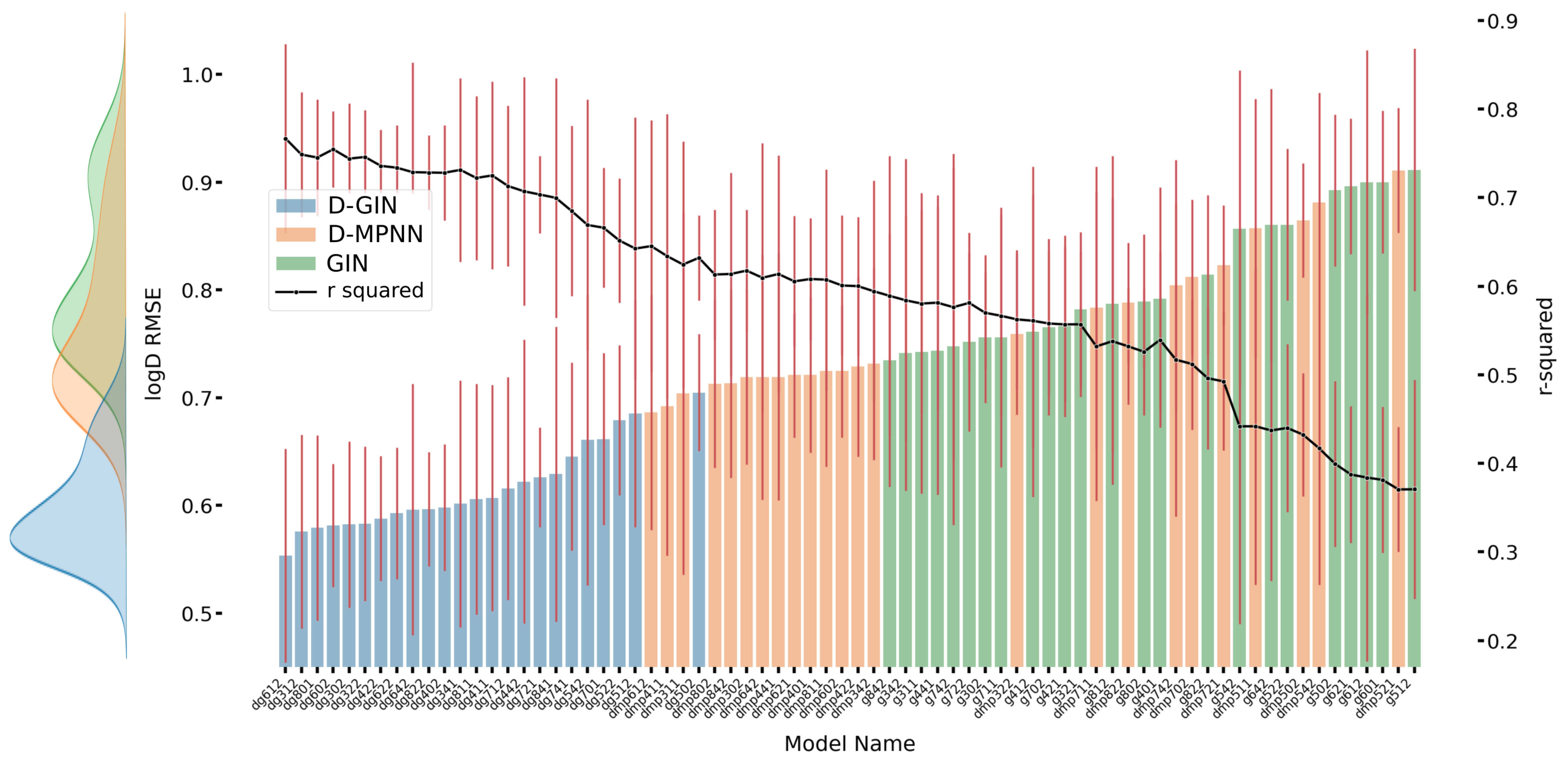
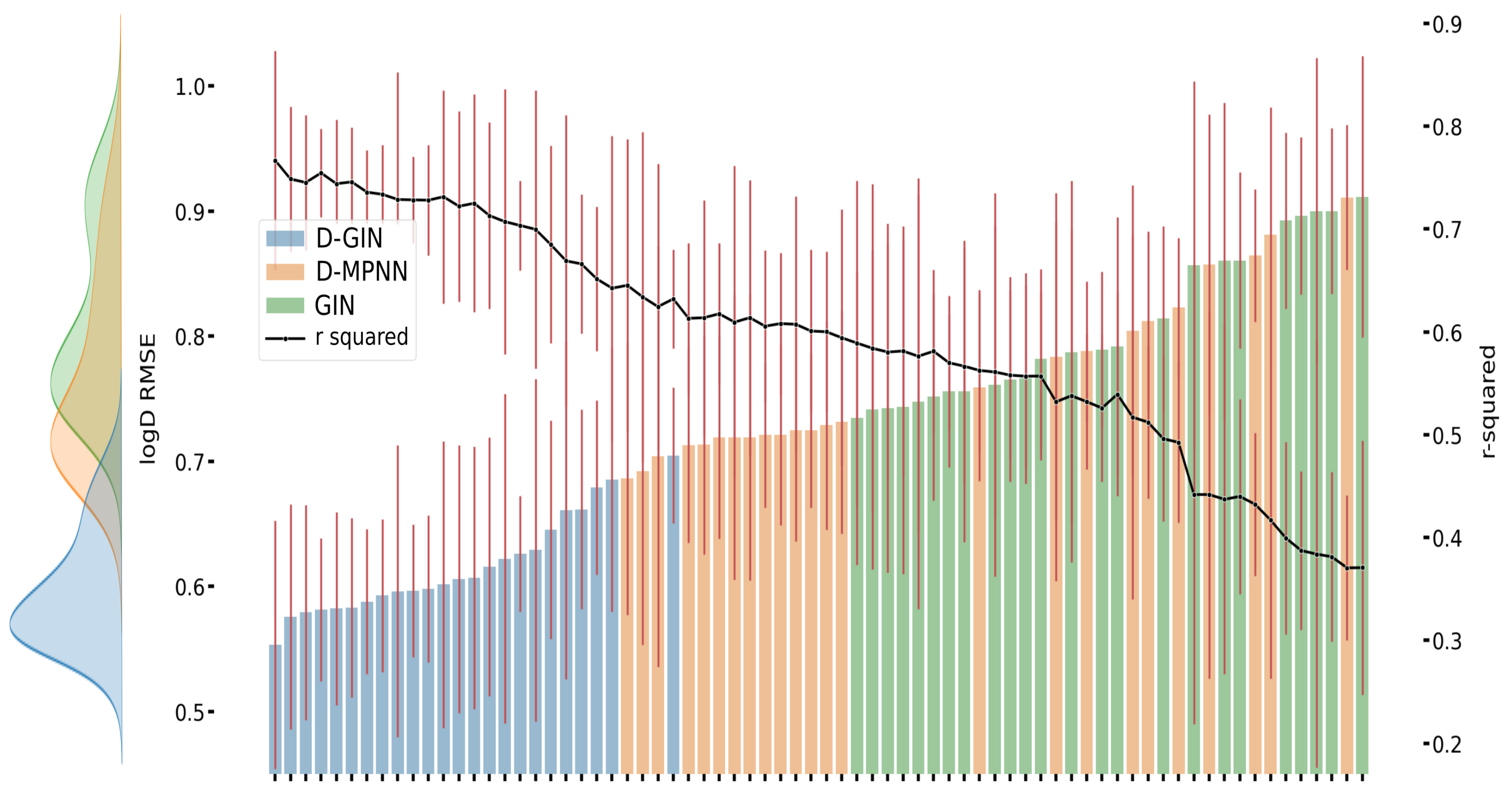
Figure A1.
The first y-axis specifies the logD RMSE and the secondary x-axis the corresponding
values for each GNN model. The D-GIN is colored blue, the D-MPNN orange and the GIN green. Each of the boxes represents one different model run. The kernel density of each model is shown on the very left side. The red lines correspond to the 95% confidence intervals. The model names are a combination of model type (D-GIN, GIN, D-MPNN), training approach and featurization type-a detailed description of each model name can be found in
Table A8,
Table A9,
Table A10,
Table A11,
Table A12,
Table A13,
Table A14,
Table A15,
Table A16,
Table A17,
Table A18 and
Table A19 in the
Appendix A.
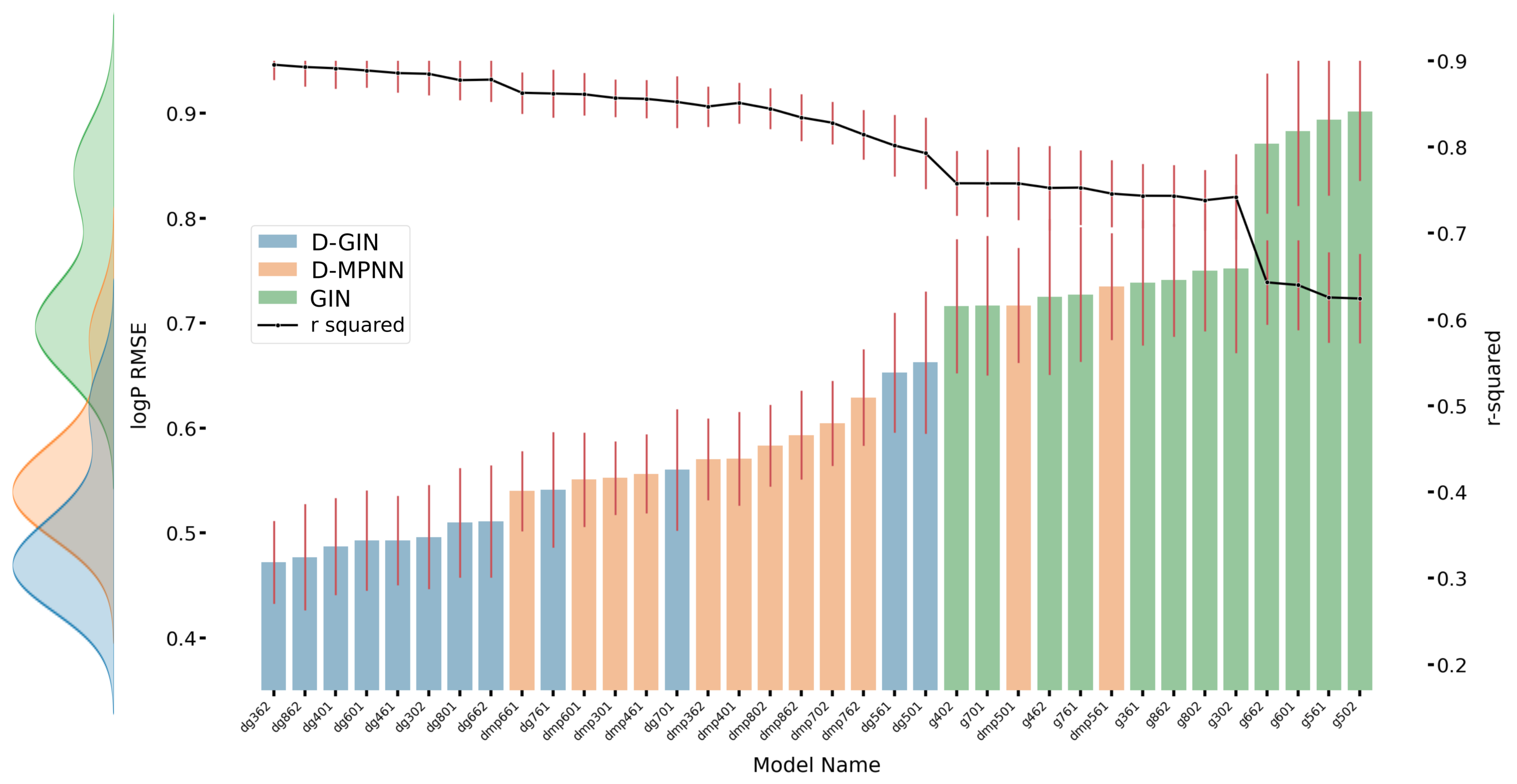
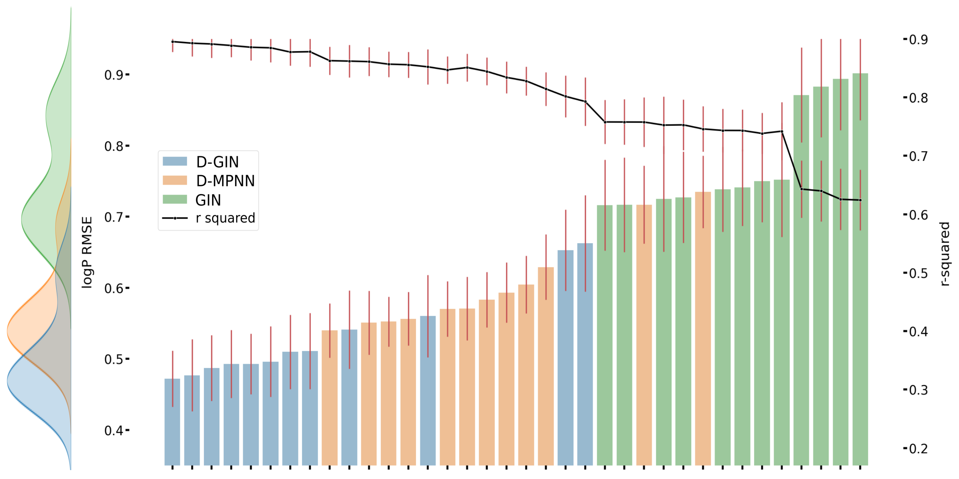
Figure A2.
The first y-axis specifies the logP RMSE and the secondary x-axis the corresponding
values for each GNN model. The D-GIN is colored blue, the D-MPNN orange and the GIN green. Each of the boxes represents one different model run. The kernel density of each model is shown on the very left side. The red lines correspond to the 95% confidence intervals. The model names are a combination of model type (D-GIN, GIN, D-MPNN), training approach and featurization type-a detailed description of each model name can be found in
Table A8,
Table A9,
Table A10,
Table A11,
Table A12,
Table A13,
Table A14,
Table A15,
Table A16,
Table A17,
Table A18 and
Table A19 in the
Appendix A.
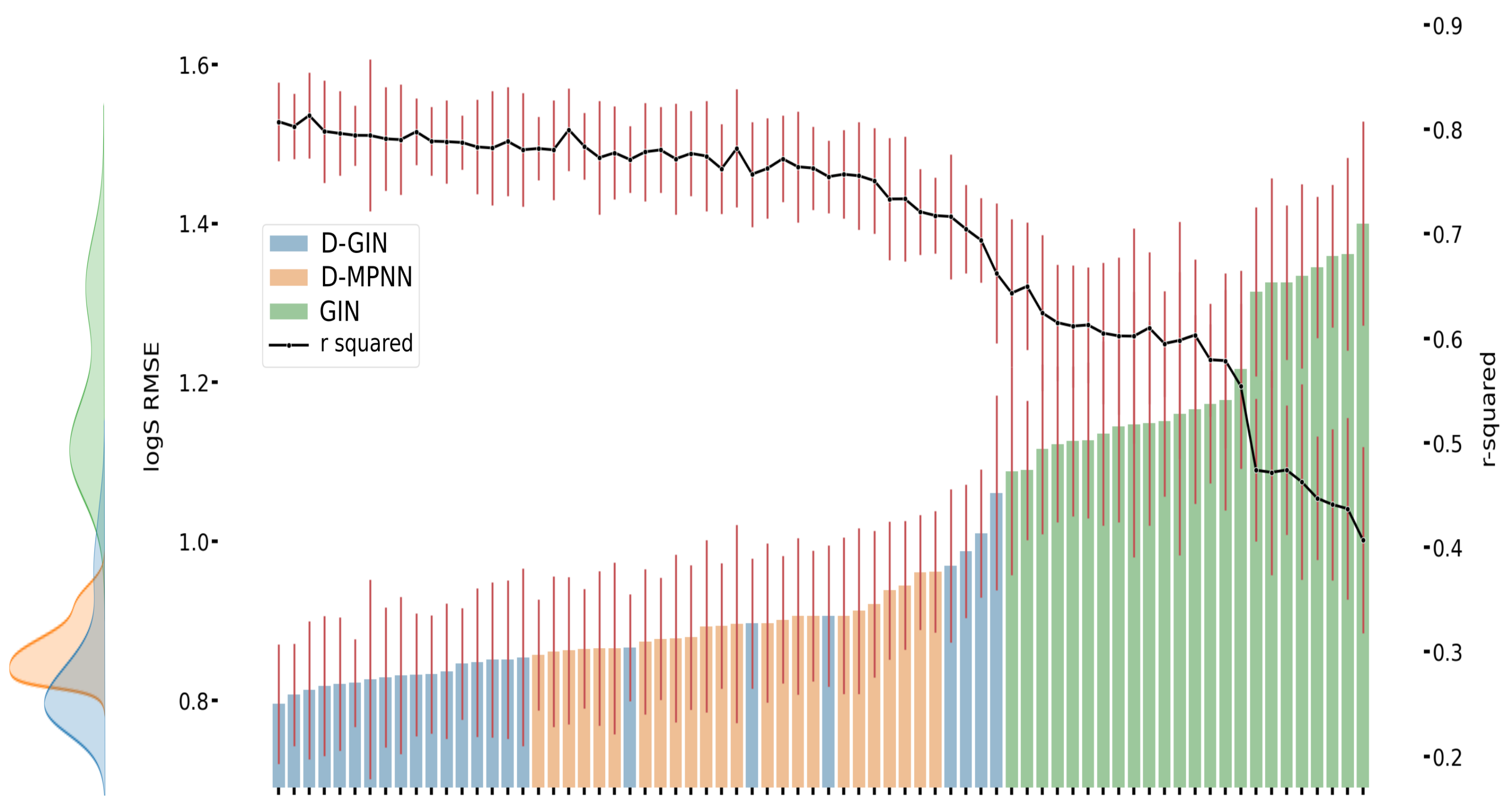
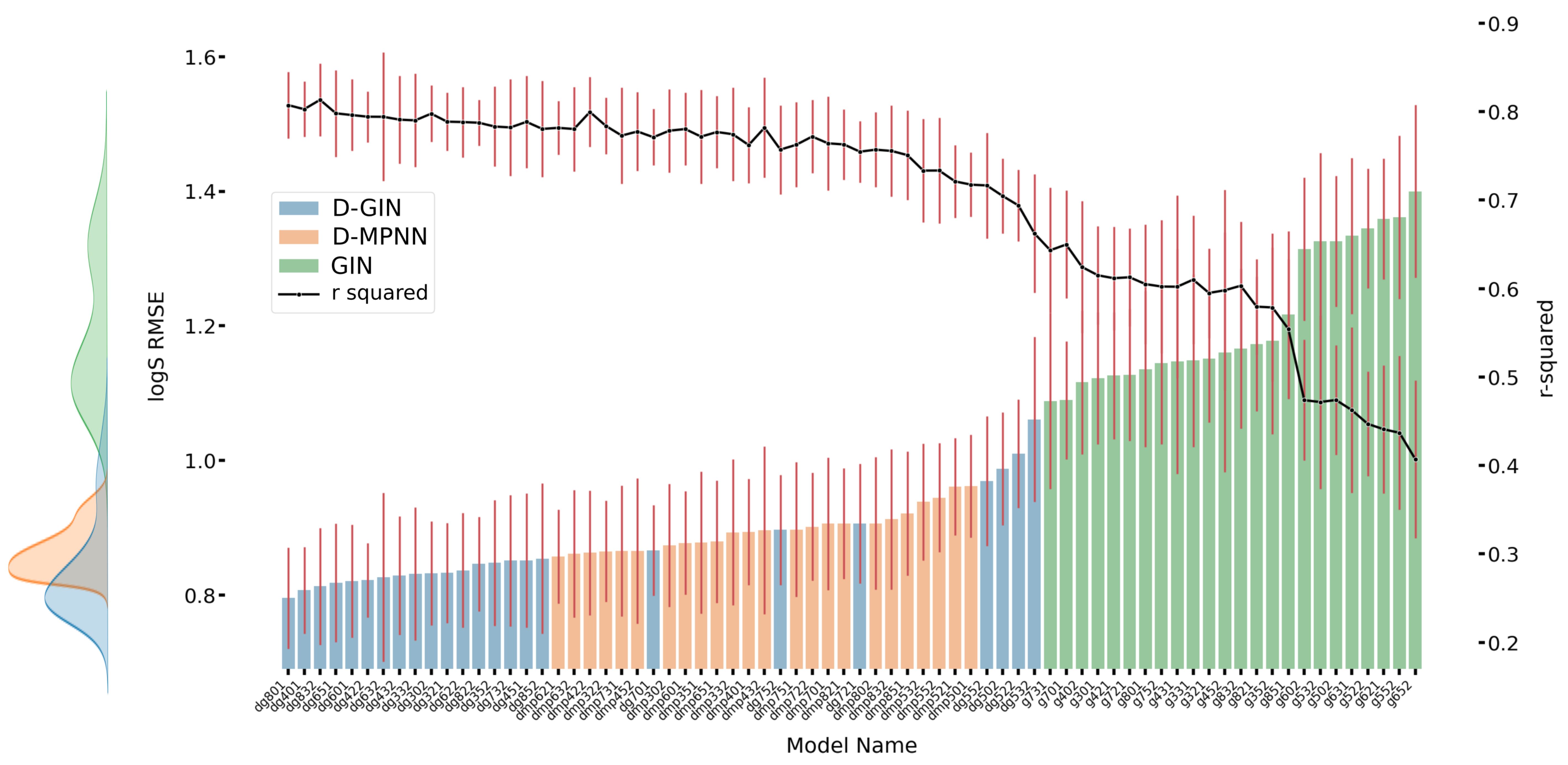
Figure A3.
The first y-axis specifies the logS RMSE and the secondary x-axis the corresponding
values for each GNN model. The D-GIN is colored blue, the D-MPNN orange and the GIN green. Each of the boxes represents one different model run. The kernel density of each model is shown on the very left side. The red lines correspond to the 95% confidence intervals. The model names are a combination of model type (D-GIN, GIN, D-MPNN), training approach and featurization type-a detailed description of each model name can be found in
Table A8,
Table A9,
Table A10,
Table A11,
Table A12,
Table A13,
Table A14,
Table A15,
Table A16,
Table A17,
Table A18 and
Table A19 in the
Appendix A.
Table A8.
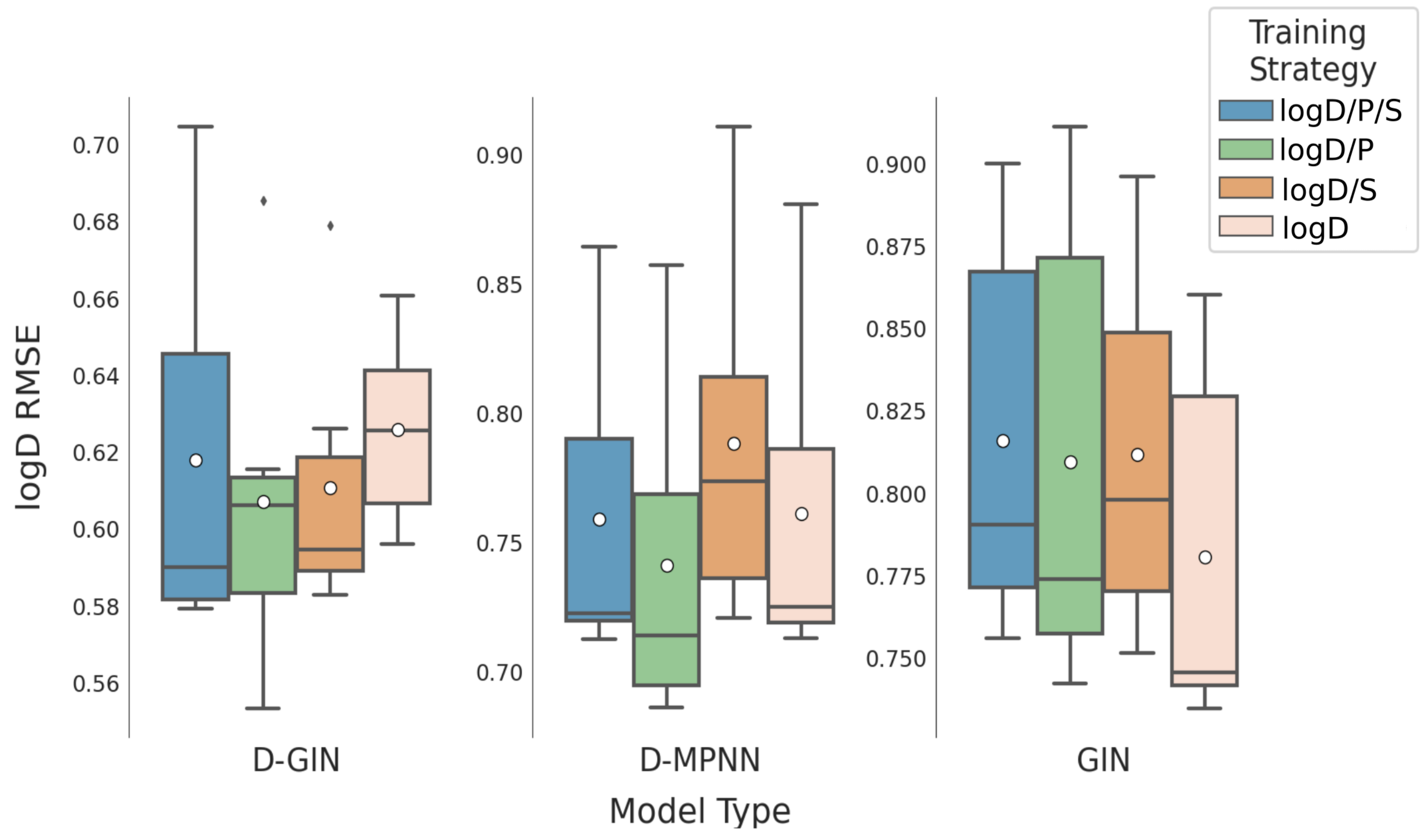
Shows the log D RMSE and results for the D-GIN model type used during this survey. The last column consist of the unique identify. Training strategy 0 represents a training strategy combining logD, logS, and logP, 1 represents a strategy combining logD and logP, 2 stands for a combination of logD and logS, 3 represents a strategy using logS and logP, 4 represents a strategy using logD, 5 represents a strategy using logS, and 6 represents a strategy using logP.
Table A8.
Shows the log D RMSE and results for the D-GIN model type used during this survey. The last column consist of the unique identify. Training strategy 0 represents a training strategy combining logD, logS, and logP, 1 represents a strategy combining logD and logP, 2 stands for a combination of logD and logS, 3 represents a strategy using logS and logP, 4 represents a strategy using logD, 5 represents a strategy using logS, and 6 represents a strategy using logP.
| Model | Training | Featurization | logD | | Unique |
|---|
| Type | Strategy | Strategy | RMSE | | ID |
|---|
| D-GIN | 2 | 5 | 0.679 ± 0.034 | 0.652 ± 0.035 | dg522 |
| D-GIN | 2 | 8 | 0.596 ± 0.026 | 0.728 ± 0.021 | dg822 |
| D-GIN | 2 | 4 | 0.587 ± 0.029 | 0.736 ± 0.020 | dg422 |
| D-GIN | 2 | 3 | 0.582 ± 0.035 | 0.746 ± 0.027 | dg322 |
| D-GIN | 0 | 3 | 0.582 ± 0.038 | 0.744 ± 0.031 | dg302 |
| D-GIN | 0 | 6 | 0.581 ± 0.028 | 0.755 ± 0.021 | dg602 |
| D-GIN | 0 | 4 | 0.598 ± 0.029 | 0.728 ± 0.027 | dg402 |
| D-GIN | 4 | 3 | 0.601 ± 0.057 | 0.731 ± 0.052 | dg341 |
| D-GIN | 0 | 8 | 0.579 ± 0.043 | 0.745 ± 0.033 | dg801 |
| D-GIN | 1 | 3 | 0.575 ± 0.044 | 0.749 ± 0.035 | dg312 |
| D-GIN | 1 | 8 | 0.605 ± 0.053 | 0.722 ± 0.046 | dg811 |
| D-GIN | 4 | 6 | 0.596 ± 0.058 | 0.729 ± 0.062 | dg642 |
| D-GIN | 1 | 4 | 0.606 ± 0.052 | 0.725 ± 0.053 | dg411 |
| D-GIN | 1 | 7 | 0.615 ± 0.051 | 0.713 ± 0.045 | dg712 |
| D-GIN | 4 | 4 | 0.622 ± 0.065 | 0.707 ± 0.065 | dg442 |
| D-GIN | 2 | 7 | 0.626 ± 0.023 | 0.704 ± 0.022 | dg721 |
| D-GIN | 4 | 8 | 0.629 ± 0.068 | 0.700 ± 0.068 | dg841 |
| D-GIN | 4 | 7 | 0.645 ± 0.043 | 0.685 ± 0.048 | dg741 |
| D-GIN | 4 | 5 | 0.660 ± 0.067 | 0.669 ± 0.071 | dg542 |
| D-GIN | 0 | 7 | 0.661 ± 0.039 | 0.666 ± 0.034 | dg701 |
| D-GIN | 1 | 5 | 0.685 ± 0.052 | 0.643 ± 0.074 | dg512 |
| D-GIN | 1 | 6 | 0.553 ± 0.049 | 0.767 ± 0.053 | dg612 |
| D-GIN | 0 | 5 | 0.704 ± 0.027 | 0.632 ± 0.024 | dg502 |
| D-GIN | 2 | 6 | 0.592 ± 0.030 | 0.734 ± 0.024 | dg622 |
| D-GIN cons. | 2 | 5 | 0.605 ± 0.032 | 0.719 ± 0.031 | dg522_cons |
| D-GIN cons. | 0 | 5 | 0.622 ± 0.030 | 0.704 ± 0.027 | dg502_cons |
| D-GIN cons. | 0 | 7 | 0.603 ± 0.030 | 0.722 ± 0.025 | dg701_cons |
| D-GIN cons. | 1 | 5 | 0.609 ± 0.056 | 0.714 ± 0.062 | dg512_cons |
| D-GIN cons. | 1 | 6 | 0.548 ± 0.051 | 0.769 ± 0.049 | dg612_cons |
| D-GIN cons. | 4 | 7 | 0.589 ± 0.045 | 0.734 ± 0.043 | dg741_cons |
| D-GIN cons. | 1 | 3 | 0.561 ± 0.047 | 0.758 ± 0.039 | dg312_cons |
| D-GIN cons. | 2 | 4 | 0.557 ±0.029 | 0.762 ± 0.023 | dg422_cons |
| D-GIN cons. | 4 | 3 | 0.557 ± 0.052 | 0.762 ± 0.044 | dg341_cons |
| D-GIN cons. | 2 | 3 | 0.549 ± 0.034 | 0.769 ± 0.026 | dg322_cons |
| D-GIN cons. | 4 | 5 | 0.590 ± 0.059 | 0.733 ± 0.055 | dg542_cons |
| D-GIN cons. | 0 | 8 | 0.562 ± 0.032 | 0.758 ± 0.025 | dg801_cons |
| D-GIN cons. | 0 | 4 | 0.563 ± 0.031 | 0.757 ± 0.027 | dg402_cons |
| D-GIN cons. | 1 | 7 | 0.566 ± 0.055 | 0.754 ± 0.044 | dg712_cons |
| D-GIN cons. | 1 | 4 | 0.567 ± 0.051 | 0.754 ± 0.041 | dg411_cons |
| D-GIN cons. | 0 | 3 | 0.562 ± 0.033 | 0.758 ± 0.024 | dg302_cons |
| D-GIN cons. | 4 | 8 | 0.575 ± 0.052 | 0.746 ± 0.053 | dg841_cons |
| D-GIN cons. | 2 | 8 | 0.568 ± 0.030 | 0.753 ± 0.026 | dg821_cons |
| D-GIN cons. | 2 | 7 | 0.580 ± 0.027 | 0.742 ± 0.023 | dg721_cons |
| D-GIN cons. | 1 | 8 | 0.580 ± 0.053 | 0.742 ± 0.047 | dg811_cons |
| D-GIN cons. | 4 | 4 | 0.577 ± 0.052 | 0.744 ± 0.041 | dg442_cons |
| D-GIN cons. | 4 | 6 | 0.568 ± 0.054 | 0.751 ± 0.051 | dg642_cons |
| D-GIN cons. | 0 | 6 | 0.569 ± 0.029 | 0.751 ± 0.024 | dg602_cons |
| D-GIN cons. | 2 | 6 | 0.571 ± 0.031 | 0.750 ± 0.024 | dg622_cons |
Table A9.
Shows the logD RMSE and results for the D-MPNN model type used during this survey. The last column consists of the unique identifier. Training strategy 0 represents a training strategy combining logD, logS, and logP, 1 represents a strategy combining logD and logP, 2 stands for a combination of logD and logS, 3 represents a strategy using logS and logP, 4 represents a strategy using logD, 5 represents a strategy using logS, and 6 represents a strategy using logP.
| Model | Training | Featurization | logD | | Unique |
|---|
| Type | Strategy | Strategy | RMSE | | ID |
|---|
| D-MPNN | 1 | 7 | 0.7836 ± 0.065 | 0.532 ± 0.087 | dmp711 |
| D-MPNN | 1 | 6 | 0.686 ± 0.054 | 0.645 ± 0.071 | dmp612 |
| D-MPNN | 1 | 5 | 0.857 ± 0.060 | 0.442 ± 0.089 | dmp511 |
| D-MPNN | 2 | 3 | 0.759 ± 0.037 | 0.563 ± 0.039 | dmp322 |
| D-MPNN | 1 | 4 | 0.692 ± 0.069 | 0.634 ± 0.080 | dmp411 |
| D-MPNN | 2 | 5 | 0.911 ± 0.029 | 0.371 ± 0.035 | dmp521 |
| D-MPNN | 2 | 6 | 0.721 ± 0.029 | 0.606 ± 0.037 | dmp621 |
| D-MPNN | 0 | 4 | 0.721 ± 0.036 | 0.608 ± 0.034 | dmp401 |
| D-MPNN | 0 | 8 | 0.712 ± 0.039 | 0.613 ± 0.037 | dmp802 |
| D-MPNN | 4 | 8 | 0.713 ± 0.043 | 0.614 ± 0.057 | dmp842 |
| D-MPNN | 1 | 8 | 0.724 ± 0.044 | 0.607 ± 0.062 | dmp811 |
| D-MPNN | 4 | 4 | 0.719 ± 0.057 | 0.614 ± 0.067 | dmp441 |
| D-MPNN | 4 | 6 | 0.719 ± 0.056 | 0.610 ± 0.076 | dmp642 |
| D-MPNN | 4 | 3 | 0.731 ± 0.044 | 0.594 ± 0.062 | dmp342 |
| D-MPNN | 0 | 6 | 0.724 ± 0.030 | 0.601 ± 0.040 | dmp602 |
| D-MPNN | 1 | 3 | 0.703 ± 0.084 | 0.625 ± 0.069 | dmp311 |
| D-MPNN | 0 | 3 | 0.719 ± 0.040 | 0.618 ± 0.034 | dmp302 |
| D-MPNN | 2 | 8 | 0.788 ± 0.027 | 0.532 ± 0.033 | dmp822 |
| D-MPNN | 2 | 4 | 0.728 ± 0.041 | 0.600 ± 0.039 | dmp422 |
| D-MPNN | 2 | 7 | 0.823 ± 0.027 | 0.493 ± 0.039 | dmp721 |
| D-MPNN | 4 | 7 | 0.804 ± 0.058 | 0.517 ± 0.089 | dmp742 |
| D-MPNN | 4 | 5 | 0.881 ± 0.051 | 0.417 ± 0.077 | dmp542 |
| D-MPNN | 0 | 7 | 0.812 ± 0.035 | 0.512 ± 0.037 | dmp702 |
| D-MPNN | 0 | 5 | 0.864 ± 0.026 | 0.432 ± 0.035 | dmp502 |
| D-MPNN cons. | 0 | 4 | 0.633 ± 0.031 | 0.693 ± 0.025 | dmp402_cons |
| D-MPNN cons. | 4 | 5 | 0.699 ± 0.047 | 0.625 ± 0.056 | dmp542_cons |
| D-MPNN cons. | 2 | 4 | 0.632 ± 0.031 | 0.694 ± 0.028 | dmp422_cons |
| D-MPNN cons. | 2 | 6 | 0.632 ± 0.029 | 0.694 ± 0.028 | dmp621_cons |
| D-MPNN cons. | 2 | 5 | 0.710 ± 0.027 | 0.614 ± 0.024 | dmp521_cons |
| D-MPNN cons. | 1 | 8 | 0.632 ± 0.050 | 0.693 ± 0.058 | dmp811_cons |
| D-MPNN cons. | 0 | 3 | 0.625 ± 0.030 | 0.701 ± 0.026 | dmp302_cons |
| D-MPNN cons. | 4 | 4 | 0.625 ± 0.054 | 0.700 ± 0.052 | dmp441_cons |
| D-MPNN cons. | 1 | 3 | 0.625 ± 0.057 | 0.700 ± 0.050 | dmp311_cons |
| D-MPNN cons. | 0 | 8 | 0.624 ± 0.029 | 0.701 ± 0.023 | dmp802_cons |
| D-MPNN cons. | 4 | 8 | 0.622 ± 0.045 | 0.703 ± 0.050 | dmp842_cons |
| D-MPNN cons. | 1 | 6 | 0.618 ± 0.045 | 0.706 ± 0.051 | dmp612_cons |
| D-MPNN cons. | 1 | 4 | 0.613 ± 0.055 | 0.711 ± 0.057 | dmp411_cons |
| D-MPNN cons. | 4 | 6 | 0.634 ± 0.055 | 0.691 ± 0.066 | dmp642_cons |
| D-MPNN cons. | 0 | 6 | 0.636 ± 0.030 | 0.690 ± 0.029 | dmp602_cons |
| D-MPNN cons. | 2 | 3 | 0.646 ± 0.032 | 0.680 ± 0.028 | dmp322_cons |
| D-MPNN cons. | 1 | 5 | 0.688 ± 0.059 | 0.637 ± 0.057 | dmp512_cons |
| D-MPNN cons. | 2 | 8 | 0.652 ± 0.030 | 0.674 ± 0.025 | dmp822_cons |
| D-MPNN cons. | 1 | 7 | 0.654 ± 0.060 | 0.671 ± 0.069 | dmp711_cons |
| D-MPNN cons. | 4 | 7 | 0.663 ± 0.045 | 0.662 ± 0.058 | dmp742_cons |
| D-MPNN cons. | 0 | 7 | 0.670 ± 0.028 | 0.656 ± 0.026 | dmp701_cons |
| D-MPNN cons. | 2 | 7 | 0.674 ± 0.026 | 0.652 ± 0.029 | dmp721_cons |
| D-MPNN cons. | 0 | 5 | 0.697 ± 0.026 | 0.628 ± 0.024 | dmp502_cons |
| D-MPNN cons. | 4 | 3 | 0.636 ± 0.042 | 0.689 ± 0.055 | dmp342_cons |
Table A10.
Shows the logD RMSE and results for the GIN model type used during this survey. The last column consist of the unique identify. Training strategy 0 represents a training strategy combining logD, logS, and logP, 1 represents a strategy combining logD and logP, 2 stands for a combination of logD and logS, 3 represents a strategy using logS and logP, 4 represents a strategy using logD, 5 represents a strategy using logS, and 6 represents a strategy using logP.
| Model | Training | Featurization | logD | | Unique |
|---|
| Type | Strategy | Strategy | RMSE | | ID |
|---|
| GIN | 2 | 5 | 0.860 ± 0.035 | 0.440 ± 0.047 | g522 |
| GIN | 2 | 6 | 0.896 ± 0.031 | 0.387 ± 0.039 | g621 |
| GIN | 0 | 4 | 0.791 ± 0.051 | 0.539 ± 0.050 | g401 |
| GIN | 0 | 8 | 0.789 ± 0.031 | 0.526 ± 0.036 | g802 |
| GIN | 2 | 8 | 0.814 ± 0.036 | 0.496 ± 0.040 | g822 |
| GIN | 1 | 8 | 0.786 ± 0.068 | 0.538 ± 0.081 | g812 |
| GIN | 1 | 6 | 0.899 ± 0.061 | 0.384 ± 0.104 | g612 |
| GIN | 4 | 8 | 0.734 ± 0.058 | 0.589 ± 0.079 | g842 |
| GIN | 4 | 5 | 0.856 ± 0.073 | 0.442 ± 0.112 | g542 |
| GIN | 0 | 5 | 0.892 ± 0.035 | 0.400 ± 0.047 | g502 |
| GIN | 4 | 3 | 0.741 ± 0.063 | 0.584 ± 0.080 | g342 |
| GIN | 1 | 7 | 0.756 ± 0.060 | 0.567 ± 0.057 | g711 |
| GIN | 1 | 4 | 0.761 ± 0.076 | 0.561 ± 0.071 | g412 |
| GIN | 4 | 4 | 0.743 ± 0.066 | 0.581 ± 0.061 | g441 |
| GIN | 4 | 7 | 0.747 ± 0.082 | 0.576 ± 0.087 | g742 |
| GIN | 2 | 7 | 0.751 ± 0.041 | 0.581 ± 0.040 | g722 |
| GIN | 2 | 3 | 0.781 ± 0.035 | 0.557 ± 0.041 | g321 |
| GIN | 2 | 4 | 0.766 ± 0.042 | 0.557 ± 0.044 | g421 |
| GIN | 0 | 7 | 0.765 ± 0.040 | 0.558 ± 0.041 | g702 |
| GIN | 0 | 3 | 0.756 ± 0.030 | 0.570 ± 0.033 | g302 |
| GIN | 1 | 3 | 0.742 ± 0.065 | 0.580 ± 0.062 | g311 |
| GIN | 4 | 6 | 0.860 ± 0.063 | 0.437 ± 0.085 | g642 |
| GIN | 0 | 6 | 0.900 ± 0.033 | 0.381 ± 0.041 | g601 |
| GIN | 1 | 5 | 0.911 ± 0.056 | 0.371 ± 0.062 | g512 |
| GINcons. | 0 | 6 | 0.715 ± 0.020 | 0.609 ± 0.025 | g602_cons |
| GINcons. | 4 | 3 | 0.627 ± 0.054 | 0.698 ± 0.059 | g342_cons |
| GINcons. | 4 | 8 | 0.632 ± 0.050 | 0.693 ± 0.057 | g842_cons |
| GINcons. | 4 | 7 | 0.633 ± 0.061 | 0.692 ± 0.056 | g742_cons |
| GINcons. | 4 | 4 | 0.637 ± 0.058 | 0.688 ± 0.060 | g441_cons |
| GINcons. | 1 | 3 | 0.640 ± 0.056 | 0.685 ± 0.051 | g311_cons |
| GINcons. | 2 | 7 | 0.642 ± 0.033 | 0.685 ± 0.028 | g722_cons |
| GINcons. | 1 | 7 | 0.644 ± 0.047 | 0.682 ± 0.053 | g711_cons |
| GINcons. | 2 | 4 | 0.645 ± 0.034 | 0.681 ± 0.031 | g421_cons |
| GINcons. | 0 | 3 | 0.647 ± 0.029 | 0.679 ± 0.025 | g302_cons |
| GINcons. | 1 | 4 | 0.648 ± 0.059 | 0.678 ± 0.056 | g412_cons |
| GINcons. | 0 | 4 | 0.652 ± 0.033 | 0.674 ± 0.030 | g401_cons |
| GINcons. | 0 | 7 | 0.654 ± 0.029 | 0.673 ± 0.024 | g701_cons |
| GINcons. | 2 | 3 | 0.656 ± 0.028 | 0.670 ± 0.030 | g321_cons |
| GINcons. | 1 | 8 | 0.657 ± 0.055 | 0.669 ± 0.068 | g812_cons |
| GINcons. | 0 | 8 | 0.661 ± 0.034 | 0.665 ± 0.031 | g801_cons |
| GINcons. | 2 | 8 | 0.673 ± 0.032 | 0.653 ± 0.029 | g822_cons |
| GINcons. | 4 | 5 | 0.689 ± 0.056 | 0.636 ± 0.064 | g542_cons |
| GINcons. | 4 | 6 | 0.692 ± 0.052 | 0.633 ± 0.057 | g642_cons |
| GINcons. | 1 | 6 | 0.707 ± 0.057 | 0.616 ± 0.061 | g612_cons |
| GINcons. | 2 | 6 | 0.707 ± 0.025 | 0.617 ± 0.025 | g622_cons |
| GINcons. | 0 | 5 | 0.712 ± 0.033 | 0.612 ± 0.030 | g502_cons |
| GINcons. | 1 | 5 | 0.719 ± 0.046 | 0.603 ± 0.052 | g512_cons |
| GINcons. | 2 | 5 | 0.692 ± 0.026 | 0.634 ± 0.022 | g522_cons |
Table A11.
Shows the logD RMSE and results for the non-GNN model types used during this survey. The last column consists of the unique identifier. Training strategy 0 represents a training strategy combining logD, logS, and logP, 1 represents a strategy combining logD and logP, 2 stands for a combination of logD and logS, 3 represents a strategy using logS and logP, 4 represents a strategy using logD, 5 represents a strategy using logS, and 6 represents a strategy using logP.
| Model | Training | Featurization | logD | | Unique |
|---|
| Type | Strategy | Strategy | RMSE | | ID |
|---|
| KNN | logD | 10 | 0.979 ± 0.072 | 0.261 ± 0.094 | KNN10 |
| KNN | logD | 16 | 0.970 ± 0.056 | 0.275 ± 0.097 | KNN16 |
| KNN | logD | 12 | 0.959 ± 0.066 | 0.293 ± 0.080 | KNN12 |
| KNN | logD | 11 | 0.993 ± 0.072 | 0.240 ± 0.096 | KNN11 |
| KNN | logD | 13 | 0.909 ± 0.067 | 0.363 ± 0.069 | KNN13 |
| KNN | logD | 15 | 1.003 ± 0.057 | 0.226 ± 0.096 | KNN15 |
| KNN | logD | 14 | 0.996 ± 0.065 | 0.236 ± 0.110 | KNN14 |
| KNN | logD | 17 | 0.801 ± 0.060 | 0.506 ± 0.058 | KNN17 |
| RF | logD | 17 | 0.708 ± 0.060 | 0.614 ± 0.055 | rf17 |
| RF | logD | 15 | 0.699 ± 0.062 | 0.623 ± 0.059 | rf15 |
| RF | logD | 16 | 0.703 ± 0.061 | 0.620 ± 0.057 | rf16 |
| RF | logD | 11 | 0.859 ± 0.062 | 0.433 ± 0.062 | rf11 |
| RF | logD | 14 | 0.706 ± 0.062 | 0.616 ± 0.058 | rf14 |
| RF | logD | 10 | 0.890 ± 0.060 | 0.390 ± 0.062 | rf10 |
| RF | logD | 13 | 0.813 ± 0.060 | 0.491 ± 0.059 | rf13 |
| RF | logD | 12 | 0.863 ± 0.068 | 0.427 ± 0.068 | rf12 |
| SVM | logD | 12 | 0.782 ± 0.061 | 0.529 ± 0.055 | svm12 |
| SVM | logD | 16 | 0.707 ± 0.056 | 0.615 ± 0.047 | svm16 |
| SVM | logD | 10 | 0.810 ± 0.062 | 0.495 ± 0.057 | svm10 |
| SVM | logD | 15 | 0.698 ± 0.055 | 0.625 ± 0.045 | svm15 |
| SVM | logD | 14 | 0.674 ± 0.054 | 0.650 ± 0.043 | svm14 |
| SVM | logD | 17 | 0.639 ± 0.051 | 0.686 ± 0.046 | svm17 |
| SVM | logD | 11 | 0.793 ± 0.060 | 0.516 ± 0.060 | svm11 |
| SVM | logD | 13 | 0.814 ± 0.059 | 0.490 ± 0.055 | svm13 |
Table A12.
Shows the logS RMSE and results for the D-GIN model type used during this survey. The last column consists of the unique identifier. Training strategy 0 represents a training strategy combining logD, logS, and logP, 1 represents a strategy combining logD and logP, 2 stands for a combination of logD and logS, 3 represents a strategy using logS and logP, 4 represents a strategy using logD, 5 represents a strategy using logS, and 6 represents a strategy using logP.
| Model | Training | Featurization | logD | | Unique |
|---|
| Type | Strategy | Strategy | RMSE | | ID |
|---|
| D-GIN | 5 | 7 | 0.897 ± 0.041 | 0.757 ± 0.025 | dg752 |
| D-GIN | 0 | 7 | 0.866 ± 0.034 | 0.771 ± 0.016 | dg701 |
| D-GIN | 5 | 5 | 0.969 ± 0.048 | 0.717 ± 0.030 | dg552 |
| D-GIN | 0 | 5 | 0.988 ± 0.042 | 0.705 ± 0.021 | dg502 |
| D-GIN | 2 | 5 | 1.010 ± 0.040 | 0.694 ± 0.020 | dg522 |
| D-GIN | 0 | 8 | 0.795 ± 0.038 | 0.807 ± 0.019 | dg801 |
| D-GIN | 0 | 4 | 0.807 ± 0.032 | 0.803 ± 0.016 | dg401 |
| D-GIN | 3 | 8 | 0.813 ± 0.044 | 0.813 ± 0.021 | dg832 |
| D-GIN | 5 | 6 | 0.818 ± 0.044 | 0.798 ± 0.025 | dg651 |
| D-GIN | 5 | 3 | 0.848 ± 0.047 | 0.783 ± 0.023 | dg352 |
| D-GIN | 0 | 6 | 0.821 ± 0.042 | 0.796 ± 0.020 | dg601 |
| D-GIN | 2 | 7 | 0.906 ± 0.045 | 0.755 ± 0.017 | dg721 |
| D-GIN | 2 | 4 | 0.822 ± 0.028 | 0.794 ± 0.014 | dg422 |
| D-GIN | 3 | 6 | 0.827 ± 0.063 | 0.794 ± 0.036 | dg632 |
| D-GIN | 5 | 8 | 0.854 ± 0.056 | 0.781 ± 0.027 | dg852 |
| D-GIN | 3 | 4 | 0.829 ± 0.044 | 0.791 ± 0.025 | dg432 |
| D-GIN | 3 | 3 | 0.831 ± 0.050 | 0.790 ± 0.026 | dg332 |
| D-GIN | 0 | 3 | 0.832 ± 0.039 | 0.798 ± 0.016 | dg302 |
| D-GIN | 2 | 3 | 0.833 ± 0.037 | 0.789 ± 0.016 | dg321 |
| D-GIN | 5 | 4 | 0.852 ± 0.050 | 0.789 ± 0.026 | dg451 |
| D-GIN | 3 | 7 | 0.851 ± 0.049 | 0.782 ± 0.027 | dg732 |
| D-GIN | 2 | 6 | 0.837 ± 0.042 | 0.788 ± 0.020 | dg622 |
| D-GIN | 3 | 5 | 1.061 ± 0.061 | 0.662 ± 0.034 | dg532 |
| D-GIN cons. | 2 | 5 | 0.794 ± 0.039 | 0.807 ± 0.014 | dg522_cons |
| D-GIN cons. | 0 | 5 | 0.779 ± 0.040 | 0.814 ± 0.014 | dg502_cons |
| D-GIN cons. | 5 | 5 | 0.778 ± 0.049 | 0.816 ± 0.020 | dg552_cons |
| D-GIN cons. | 3 | 5 | 0.820 ± 0.054 | 0.795 ± 0.024 | dg532_cons |
| D-GIN cons. | 0 | 8 | 0.705 ± 0.039 | 0.848 ± 0.014 | dg801_cons |
| D-GIN cons. | 2 | 7 | 0.757 ± 0.044 | 0.825 ± 0.015 | dg721_cons |
| D-GIN cons. | 2 | 8 | 0.734 ± 0.033 | 0.835 ± 0.012 | dg822_cons |
| D-GIN cons. | 3 | 7 | 0.733 ± 0.046 | 0.836 ± 0.021 | dg732_cons |
| D-GIN cons. | 0 | 3 | 0.733 ± 0.040 | 0.836 ± 0.015 | dg301_cons |
| D-GIN cons. | 0 | 7 | 0.731 ± 0.035 | 0.836 ± 0.010 | dg701_cons |
| D-GIN cons. | 5 | 3 | 0.730 ± 0.047 | 0.838 ± 0.019 | dg352_cons |
| D-GIN cons. | 3 | 3 | 0.727 ± 0.048 | 0.839 ± 0.021 | dg332_cons |
| D-GIN cons. | 5 | 4 | 0.739 ± 0.052 | 0.834 ± 0.023 | dg451_cons |
| D-GIN cons. | 5 | 7 | 0.748 ± 0.045 | 0.830 ± 0.018 | dg752_cons |
| D-GIN cons. | 2 | 3 | 0.725 ± 0.041 | 0.839 ± 0.014 | dg321_cons |
| D-GIN cons. | 3 | 8 | 0.724 ± 0.046 | 0.840 ± 0.018 | dg832_cons |
| D-GIN cons. | 3 | 4 | 0.722 ± 0.047 | 0.841 ± 0.020 | dg432_cons |
| D-GIN cons. | 2 | 4 | 0.718 ± 0.031 | 0.842 ± 0.011 | dg422_cons |
| D-GIN cons. | 3 | 6 | 0.718 ± 0.047 | 0.843 ± 0.021 | dg631_cons |
| D-GIN cons. | 2 | 6 | 0.716 ± 0.038 | 0.843 ± 0.014 | dg622_cons |
| D-GIN cons. | 0 | 4 | 0.715 ± 0.035 | 0.843 ± 0.011 | dg401_cons |
| D-GIN cons. | 5 | 6 | 0.711 ± 0.046 | 0.846 ± 0.021 | dg651_cons |
| D-GIN cons. | 0 | 6 | 0.724 ± 0.038 | 0.839 ± 0.016 | dg601_cons |
| D-GIN cons. | 5 | 8 | 0.735 ± 0.053 | 0.835 ± 0.021 | dg852_cons |
Table A13.
Shows the logS RMSE and results for the D-MPNN model type used during this survey. The last column consist of the unique identify. Training strategy 0 represents a training strategy combining logD, logS, and logP, 1 represents a strategy combining logD and logP, 2 stands for a combination of logD and logS, 3 represents a strategy using logS and logP, 4 represents a strategy using logD, 5 represents a strategy using logS, and 6 represents a strategy using logP.
| Model | Training | Featurization | logD | | Unique |
|---|
| Type | Strategy | Strategy | RMSE | | ID |
|---|
| D-MPNN | 3 | 8 | 0.913 ± 0.052 | 0.756 ± 0.026 | dmp832 |
| D-MPNN | 2 | 6 | 0.857 ± 0.035 | 0.782 ± 0.015 | dmp621 |
| D-MPNN | 2 | 3 | 0.865 ± 0.038 | 0.784 ± 0.016 | dmp322 |
| D-MPNN | 0 | 5 | 0.962 ± 0.038 | 0.718 ± 0.018 | dmp501 |
| D-MPNN | 0 | 8 | 0.907 ± 0.049 | 0.757 ± 0.021 | dmp802 |
| D-MPNN | 5 | 8 | 0.921 ± 0.046 | 0.751 ± 0.025 | dmp851 |
| D-MPNN | 2 | 8 | 0.906 ± 0.041 | 0.763 ± 0.020 | dmp821 |
| D-MPNN | 0 | 7 | 0.906 ± 0.049 | 0.764 ± 0.027 | dmp701 |
| D-MPNN | 2 | 7 | 0.902 ± 0.040 | 0.772 ± 0.021 | dmp722 |
| D-MPNN | 3 | 5 | 0.938 ± 0.044 | 0.733 ± 0.029 | dmp532 |
| D-MPNN | 5 | 5 | 0.945 ± 0.041 | 0.734 ± 0.030 | dmp552 |
| D-MPNN | 3 | 4 | 0.896 ± 0.062 | 0.782 ± 0.028 | dmp432 |
| D-MPNN | 0 | 4 | 0.893 ± 0.040 | 0.762 ± 0.022 | dmp401 |
| D-MPNN | 3 | 3 | 0.893 ± 0.054 | 0.775 ± 0.026 | dmp332 |
| D-MPNN | 5 | 6 | 0.879 ± 0.046 | 0.777 ± 0.021 | dmp651 |
| D-MPNN | 5 | 3 | 0.878 ± 0.053 | 0.772 ± 0.027 | dmp351 |
| D-MPNN | 0 | 6 | 0.877 ± 0.039 | 0.780 ± 0.021 | dmp601 |
| D-MPNN | 0 | 3 | 0.874 ± 0.046 | 0.779 ± 0.024 | dmp302 |
| D-MPNN | 2 | 5 | 0.961 ± 0.036 | 0.721 ± 0.021 | dmp521 |
| D-MPNN | 5 | 4 | 0.866 ± 0.054 | 0.778 ± 0.022 | dmp452 |
| D-MPNN | 3 | 7 | 0.865 ± 0.049 | 0.773 ± 0.027 | dmp731 |
| D-MPNN | 2 | 4 | 0.863 ± 0.046 | 0.800 ± 0.020 | dmp422 |
| D-MPNN | 5 | 7 | 0.897 ± 0.050 | 0.763 ± 0.024 | dmp751 |
| D-MPNN | 3 | 6 | 0.861 ± 0.047 | 0.780 ± 0.024 | dmp632 |
| D-MPNN cons. | 5 | 4 | 0.748 ± 0.055 | 0.830 ± 0.020 | dmp452_cons |
| D-MPNN cons. | 0 | 4 | 0.768 ± 0.040 | 0.819 ± 0.015 | dmp401_cons |
| D-MPNN cons. | 2 | 8 | 0.769 ± 0.039 | 0.819 ± 0.014 | dmp821_cons |
| D-MPNN cons. | 3 | 8 | 0.762 ± 0.052 | 0.823 ± 0.022 | dmp832_cons |
| D-MPNN cons. | 5 | 6 | 0.749 ± 0.053 | 0.829 ± 0.021 | dmp652_cons |
| D-MPNN cons. | 0 | 8 | 0.770 ± 0.044 | 0.818 ± 0.016 | dmp802_cons |
| D-MPNN cons. | 3 | 3 | 0.762 ± 0.052 | 0.823 ± 0.021 | dmp332_cons |
| D-MPNN cons. | 0 | 7 | 0.771 ± 0.044 | 0.818 ± 0.016 | dmp701_cons |
| D-MPNN cons. | 2 | 7 | 0.771 ± 0.040 | 0.818 ± 0.016 | dmp722_cons |
| D-MPNN cons. | 5 | 7 | 0.761 ± 0.051 | 0.824 ± 0.021 | dmp751_cons |
| D-MPNN cons. | 5 | 8 | 0.774 ± 0.048 | 0.817 ± 0.022 | dmp851_cons |
| D-MPNN cons. | 3 | 5 | 0.777 ± 0.048 | 0.816 ± 0.021 | dmp532_cons |
| D-MPNN cons. | 5 | 5 | 0.779 ± 0.045 | 0.815 ± 0.021 | dmp552_cons |
| D-MPNN cons. | 3 | 4 | 0.765 ± 0.056 | 0.822 ± 0.021 | dmp431_cons |
| D-MPNN cons. | 2 | 5 | 0.784 ± 0.038 | 0.811 ± 0.016 | dmp521_cons |
| D-MPNN cons. | 0 | 3 | 0.760 ± 0.042 | 0.823 ± 0.016 | dmp302_cons |
| D-MPNN cons. | 0 | 6 | 0.759 ± 0.039 | 0.823 ± 0.014 | dmp601_cons |
| D-MPNN cons. | 2 | 3 | 0.756 ± 0.039 | 0.825 ± 0.014 | dmp322_cons |
| D-MPNN cons. | 2 | 6 | 0.744 ± 0.038 | 0.831 ± 0.013 | dmp621_cons |
| D-MPNN cons. | 5 | 3 | 0.752 ± 0.055 | 0.828 ± 0.021 | dmp351_cons |
| D-MPNN cons. | 3 | 7 | 0.744 ± 0.053 | 0.831 ± 0.021 | dmp731_cons |
| D-MPNN cons. | 2 | 4 | 0.750 ± 0.044 | 0.828 ± 0.016 | dmp422_cons |
| D-MPNN cons. | 3 | 6 | 0.748 ± 0.055 | 0.830 ± 0.021 | dmp632_cons |
| D-MPNN cons. | 0 | 5 | 0.785 ± 0.040 | 0.811 ± 0.015 | dmp501_cons |
Table A14.
Shows the logS RMSE and results for the GIN model type used during this survey. The last column consists of the unique identifier. Training strategy 0 represents a training strategy combining logD, logS, and logP, 1 represents a strategy combining logD and logP, 2 stands for a combination of logD and logS, 3 represents a strategy using logS and logP, 4 represents a strategy using logD, 5 represents a strategy using logS, and 6 represents a strategy using logP.
| Model | Training | Featurization | logD | | Unique |
|---|
| Type | Strategy | Strategy | RMSE | | ID |
|---|
| GIN | 2 | 4 | 1.126 ± 0.047 | 0.612 ± 0.029 | g421 |
| GIN | 0 | 3 | 1.122 ± 0.049 | 0.615 ± 0.028 | g301 |
| GIN | 0 | 4 | 1.116 ± 0.053 | 0.624 ± 0.037 | g402 |
| GIN | 0 | 7 | 1.089 ± 0.044 | 0.650 ± 0.031 | g701 |
| GIN | 3 | 7 | 1.088 ± 0.066 | 0.643 ± 0.036 | g731 |
| GIN | 2 | 7 | 1.127 ± 0.049 | 0.613 ± 0.028 | g721 |
| GIN | 3 | 4 | 1.147 ± 0.084 | 0.602 ± 0.052 | g431 |
| GIN | 5 | 7 | 1.145 ± 0.060 | 0.602 ± 0.038 | g752 |
| GIN | 5 | 6 | 1.400 ± 0.064 | 0.407 ± 0.045 | g652 |
| GIN | 5 | 5 | 1.362 ± 0.061 | 0.437 ± 0.043 | g552 |
| GIN | 2 | 6 | 1.359 ± 0.045 | 0.441 ± 0.036 | g621 |
| GIN | 2 | 5 | 1.345 ± 0.044 | 0.447 ± 0.030 | g522 |
| GIN | 3 | 6 | 1.334 ± 0.058 | 0.463 ± 0.047 | g631 |
| GIN | 0 | 5 | 1.326 ± 0.049 | 0.474 ± 0.031 | g502 |
| GIN | 0 | 8 | 1.136 ± 0.058 | 0.605 ± 0.034 | g801 |
| GIN | 3 | 5 | 1.326 ± 0.066 | 0.472 ± 0.049 | g532 |
| GIN | 5 | 8 | 1.217 ± 0.062 | 0.554 ± 0.040 | g851 |
| GIN | 5 | 3 | 1.178 ± 0.070 | 0.579 ± 0.042 | g352 |
| GIN | 2 | 8 | 1.173 ± 0.050 | 0.580 ± 0.027 | g821 |
| GIN | 3 | 8 | 1.166 ± 0.059 | 0.603 ± 0.036 | g832 |
| GIN | 5 | 4 | 1.161 ± 0.089 | 0.598 ± 0.057 | g452 |
| GIN | 2 | 3 | 1.151 ± 0.047 | 0.595 ± 0.025 | g321 |
| GIN | 3 | 3 | 1.148 ± 0.064 | 0.610 ± 0.036 | g331 |
| GIN | 0 | 6 | 1.314 ± 0.053 | 0.474 ± 0.034 | g602 |
| GINcons. | 5 | 6 | 0.969 ± 0.057 | 0.714 ± 0.029 | g652_cons |
| GINcons. | 2 | 7 | 0.840 ± 0.036 | 0.784 ± 0.014 | g721_cons |
| GINcons. | 5 | 5 | 0.945 ± 0.045 | 0.728 ± 0.023 | g552_cons |
| GINcons. | 0 | 3 | 0.842 ± 0.041 | 0.783 ± 0.016 | g301_cons |
| GINcons. | 5 | 4 | 0.861 ± 0.065 | 0.774 ± 0.031 | g452_cons |
| GINcons. | 2 | 8 | 0.867 ± 0.043 | 0.770 ± 0.017 | g821_cons |
| GINcons. | 5 | 3 | 0.872 ± 0.056 | 0.769 ± 0.026 | g352_cons |
| GINcons. | 3 | 3 | 0.857 ± 0.054 | 0.776 ± 0.024 | g331_cons |
| GINcons. | 0 | 7 | 0.825 ± 0.038 | 0.791 ± 0.016 | g701_cons |
| GINcons. | 5 | 8 | 0.887 ± 0.056 | 0.760 ± 0.026 | g851_cons |
| GINcons. | 2 | 3 | 0.855 ± 0.043 | 0.776 ± 0.015 | g321_cons |
| GINcons. | 5 | 7 | 0.854 ± 0.055 | 0.778 ± 0.026 | g752_cons |
| GINcons. | 3 | 7 | 0.828 ± 0.052 | 0.791 ± 0.023 | g731_cons |
| GINcons. | 0 | 4 | 0.835 ± 0.040 | 0.786 ± 0.016 | g402_cons |
| GINcons. | 3 | 4 | 0.860 ± 0.061 | 0.775 ± 0.029 | g431_cons |
| GINcons. | 2 | 4 | 0.835 ± 0.041 | 0.786 ± 0.014 | g421_cons |
| GINcons. | 0 | 6 | 0.926 ± 0.045 | 0.737 ± 0.017 | g602_cons |
| GINcons. | 0 | 5 | 0.933 ± 0.038 | 0.733 ± 0.015 | g502_cons |
| GINcons. | 3 | 5 | 0.934 ± 0.053 | 0.734 ± 0.025 | g532_cons |
| GINcons. | 2 | 5 | 0.938 ± 0.040 | 0.730 ± 0.015 | g522_cons |
| GINcons. | 3 | 6 | 0.940 ± 0.048 | 0.731 ± 0.025 | g631_cons |
| GINcons. | 2 | 6 | 0.945 ± 0.041 | 0.726 ± 0.017 | g621_cons |
| GINcons. | 0 | 8 | 0.850 ± 0.042 | 0.779 ± 0.014 | g802_cons |
| GINcons. | 3 | 8 | 0.861 ± 0.053 | 0.774 ± 0.018 | g832_cons |
Table A15.
Shows the logS RMSE and results for the non-GNN model types used during this survey. The last column consists of the unique identifier. Training strategy 0 represents a training strategy combining logD, logS, and logP, 1 represents a strategy combining logD and logP, 2 stands for a combination of logD and logS, 3 represents a strategy using logS and logP, 4 represents a strategy using logD, 5 represents a strategy using logS, and 6 represents a strategy using logP.
| Model | Training | Featurization | logD | | Unique |
|---|
| Type | Strategy | Strategy | RMSE | | ID |
|---|
| KNN | logS | 14 | 1.547 ± 0.063 | 0.268 ± 0.054 | KNN14 |
| KNN | logS | 11 | 1.587 ± 0.063 | 0.230 ± 0.054 | KNN11 |
| KNN | logS | 10 | 1.587 ± 0.064 | 0.229 ± 0.056 | KNN10 |
| KNN | logS | 12 | 1.600 ± 0.066 | 0.217 ± 0.055 | KNN12 |
| KNN | logS | 13 | 1.280 ± 0.066 | 0.499 ± 0.036 | KNN13 |
| KNN | logS | 15 | 1.676 ± 0.066 | 0.140 ± 0.068 | KNN15 |
| KNN | logS | 17 | 1.058 ± 0.055 | 0.658 ± 0.032 | KNN17 |
| KNN | logS | 16 | 1.670 ± 0.065 | 0.147 ± 0.061 | KNN16 |
| RF | logS | 12 | 1.239 ± 0.056 | 0.530 ± 0.032 | rf12 |
| RF | logS | 14 | 0.760 ± 0.043 | 0.823 ± 0.020 | rf14 |
| RF | logS | 15 | 0.764 ± 0.044 | 0.821 ± 0.022 | rf15 |
| RF | logS | 13 | 1.128 ± 0.061 | 0.611 ± 0.039 | rf13 |
| RF | logS | 16 | 0.765 ± 0.045 | 0.821 ± 0.024 | rf16 |
| RF | logS | 17 | 0.770 ± 0.049 | 0.818 ± 0.025 | rf17 |
| RF | logS | 10 | 1.284 ± 0.055 | 0.495 ± 0.033 | rf10 |
| RF | logS | 11 | 1.271 ± 0.057 | 0.506 ± 0.035 | rf11 |
| SVM | logS | 12 | 1.142 ± 0.055 | 0.601 ± 0.035 | svm12 |
| SVM | logS | 11 | 1.149 ± 0.057 | 0.596 ± 0.035 | svm11 |
| SVM | logS | 16 | 0.966 ± 0.049 | 0.715 ± 0.024 | svm16 |
| SVM | logS | 15 | 0.930 ± 0.046 | 0.735 ± 0.023 | svm15 |
| SVM | logS | 13 | 1.086 ± 0.060 | 0.639 ± 0.034 | svm13 |
| SVM | logS | 17 | 0.730 ± 0.041 | 0.837 ± 0.020 | svm17 |
| SVM | logS | 14 | 0.891 ± 0.046 | 0.757 ± 0.023 | svm14 |
| SVM | logS | 10 | 1.162 ± 0.056 | 0.587 ± 0.036 | svm10 |
Table A16.
Shows the logP RMSE and results for the D-GIN model type used during this survey. The last column consists of the unique identifier. Training strategy 0 represents a training strategy combining logD, logS, and logP, 1 represents a strategy combining logD and logP, 2 stands for a combination of logD and logS, 3 represents a strategy using logS and logP, 4 represents a strategy using logD, 5 represents a strategy using logS, and 6 represents a strategy using logP.
| Model | Training | Featurization | logD | | Unique |
|---|
| Type | Strategy | Strategy | RMSE | | ID |
|---|
| D-GIN | 0 | 8 | 0.510 ± 0.026 | 0.878 ± 0.012 | dg801 |
| D-GIN | 0 | 3 | 0.496 ± 0.025 | 0.885 ± 0.012 | dg302 |
| D-GIN | 0 | 6 | 0.493 ± 0.024 | 0.889 ± 0.010 | dg601 |
| D-GIN | 6 | 4 | 0.493 ± 0.021 | 0.886 ± 0.011 | dg461 |
| D-GIN | 6 | 7 | 0.541 ± 0.028 | 0.862 ± 0.014 | dg761 |
| D-GIN | 0 | 4 | 0.487 ± 0.023 | 0.891 ± 0.012 | dg401 |
| D-GIN | 6 | 8 | 0.477 ± 0.025 | 0.893 ± 0.011 | dg862 |
| D-GIN | 0 | 7 | 0.560 ± 0.029 | 0.852 ± 0.015 | dg701 |
| D-GIN | 0 | 5 | 0.663 ± 0.034 | 0.793 ± 0.021 | dg501 |
| D-GIN | 6 | 5 | 0.653 ± 0.029 | 0.802 ± 0.018 | dg561 |
| D-GIN | 6 | 3 | 0.472 ± 0.020 | 0.896 ± 0.009 | dg362 |
| D-GIN | 6 | 6 | 0.511 ± 0.027 | 0.878 ± 0.013 | dg662 |
| D-GIN cons. | 6 | 3 | 0.428 ± 0.026 | 0.914 ± 0.010 | dg362 cons. |
| D-GIN cons. | 6 | 5 | 0.502 ± 0.027 | 0.881 ± 0.013 | dg561 cons. |
| D-GIN cons. | 0 | 7 | 0.473 ± 0.032 | 0.894 ± 0.013 | dg701 cons. |
| D-GIN cons. | 0 | 5 | 0.515 ± 0.033 | 0.875 ± 0.014 | dg501 cons. |
| D-GIN cons. | 0 | 3 | 0.447 ± 0.030 | 0.906 ± 0.012 | dg302 cons. |
| D-GIN cons. | 6 | 8 | 0.433 ± 0.030 | 0.912 ± 0.012 | dg862 cons. |
| D-GIN cons. | 0 | 6 | 0.434 ± 0.029 | 0.911 ± 0.011 | dg601 cons. |
| D-GIN cons. | 0 | 4 | 0.439 ± 0.026 | 0.909 ± 0.011 | dg401 cons. |
| D-GIN cons. | 6 | 7 | 0.461 ± 0.027 | 0.900 ± 0.012 | dg761 cons. |
| D-GIN cons. | 0 | 8 | 0.452 ± 0.030 | 0.904 ± 0.014 | dg801 cons. |
| D-GIN cons. | 6 | 4 | 0.440 ± 0.030 | 0.909 ± 0.012 | dg461 cons. |
| D-GIN cons. | 6 | 6 | 0.442 ± 0.026 | 0.908 ± 0.011 | dg661 cons. |
Table A17.
Shows the logP RMSE and results for the D-MPNN model type used during this survey. The last column consists of the unique identifier. Training strategy 0 represents a training strategy combining logD, logS, and logP, 1 represents a strategy combining logD and logP, 2 stands for a combination of logD and logS, 3 represents a strategy using logS and logP, 4 represents a strategy using logD, 5 represents a strategy using logS, and 6 represents a strategy using logP.
| Model | Training | Featurization | logD | | Unique |
|---|
| Type | Strategy | Strategy | RMSE | | ID |
|---|
| D-MPNN | 6 | 6 | 0.540 ± 0.019 | 0.863 ± 0.012 | dmp661 |
| D-MPNN | 6 | 5 | 0.735 ± 0.026 | 0.746 ± 0.019 | dmp561 |
| D-MPNN | 0 | 8 | 0.583 ± 0.020 | 0.845 ± 0.012 | dmp802 |
| D-MPNN | 0 | 6 | 0.551 ± 0.022 | 0.861 ± 0.012 | dmp601 |
| D-MPNN | 6 | 4 | 0.556 ± 0.019 | 0.856 ± 0.011 | dmp461 |
| D-MPNN | 0 | 5 | 0.717 ± 0.027 | 0.758 ± 0.021 | dmp501 |
| D-MPNN | 6 | 3 | 0.570 ± 0.019 | 0.847 ± 0.012 | dmp362 |
| D-MPNN | 6 | 7 | 0.629 ± 0.023 | 0.815 ± 0.014 | dmp762 |
| D-MPNN | 0 | 7 | 0.605 ± 0.020 | 0.828 ± 0.012 | dmp702 |
| D-MPNN | 6 | 8 | 0.593 ± 0.021 | 0.834 ± 0.014 | dmp862 |
| D-MPNN | 0 | 4 | 0.571 ± 0.022 | 0.851 ± 0.012 | dmp401 |
| D-MPNN | 0 | 3 | 0.552 ± 0.018 | 0.857 ± 0.011 | dmp301 |
| D-MPNN cons. | 6 | 5 | 0.533 ± 0.031 | 0.866 ± 0.015 | dmp562 cons. |
| D-MPNN cons. | 0 | 6 | 0.444 ± 0.024 | 0.907 ± 0.010 | dmp601 cons. |
| D-MPNN cons. | 6 | 6 | 0.452 ± 0.026 | 0.904 ± 0.011 | dmp661 cons. |
| D-MPNN cons. | 0 | 5 | 0.524 ± 0.031 | 0.870 ± 0.015 | dmp501 cons. |
| D-MPNN cons. | 0 | 3 | 0.461 ± 0.027 | 0.900 ± 0.011 | dmp301 cons. |
| D-MPNN cons. | 0 | 4 | 0.463 ± 0.027 | 0.899 ± 0.011 | dmp401 cons. |
| D-MPNN cons. | 6 | 3 | 0.464 ± 0.026 | 0.899 ± 0.012 | dmp362 cons. |
| D-MPNN cons. | 6 | 8 | 0.471 ± 0.028 | 0.895 ± 0.012 | dmp862 cons. |
| D-MPNN cons. | 0 | 8 | 0.475 ± 0.027 | 0.894 ± 0.011 | dmp802 cons. |
| D-MPNN cons. | 0 | 7 | 0.484 ± 0.028 | 0.890 ± 0.012 | dmp701 cons. |
| D-MPNN cons. | 6 | 4 | 0.454 ± 0.026 | 0.903 ± 0.012 | dmp462 cons. |
| D-MPNN cons. | 6 | 7 | 0.488 ± 0.027 | 0.888 ± 0.012 | dmp761 cons. |
Table A18.
Shows the logP RMSE and results for the GIN model type used during this survey. The last column consists of the unique identifier. Training strategy 0 represents a training strategy combining logD, logS, and logP, 1 represents a strategy combining logD and logP, 2 stands for a combination of logD and logS, 3 represents a strategy using logS and logP, 4 represents a strategy using logD, 5 represents a strategy using logS, and 6 represents a strategy using logP.
| Model | Training | Featurization | logD | | Unique |
|---|
| Type | Strategy | Strategy | RMSE | | ID |
|---|
| GIN | 0 | 3 | 0.752 ± 0.040 | 0.742 ± 0.025 | g302 |
| GIN | 0 | 8 | 0.750 ± 0.029 | 0.738 ± 0.018 | g802 |
| GIN | 0 | 4 | 0.716 ± 0.032 | 0.758 ± 0.019 | g402 |
| GIN | 0 | 5 | 0.902 ± 0.033 | 0.624 ± 0.026 | g502 |
| GIN | 6 | 5 | 0.894 ± 0.036 | 0.626 ± 0.026 | g561 |
| GIN | 0 | 7 | 0.717 ± 0.033 | 0.758 ± 0.019 | g701 |
| GIN | 6 | 7 | 0.727 ± 0.032 | 0.753 ± 0.022 | g761 |
| GIN | 6 | 3 | 0.739 ± 0.030 | 0.744 ± 0.019 | g361 |
| GIN | 6 | 8 | 0.741 ± 0.027 | 0.743 ± 0.018 | g862 |
| GIN | 6 | 6 | 0.871 ± 0.033 | 0.643 ± 0.024 | g662 |
| GIN | 6 | 4 | 0.725 ± 0.037 | 0.753 ± 0.025 | g462 |
| GIN | 0 | 6 | 0.883 ± 0.036 | 0.640 ± 0.026 | g601 |
| GINcons. | 6 | 7 | 0.537 ± 0.035 | 0.864 ± 0.016 | g761 cons. |
| GINcons. | 6 | 8 | 0.548 ± 0.034 | 0.858 ± 0.016 | g861 cons. |
| GINcons. | 0 | 4 | 0.539 ± 0.035 | 0.863 ± 0.015 | g402 cons. |
| GINcons. | 0 | 7 | 0.539 ± 0.034 | 0.863 ± 0.015 | g701 cons. |
| GINcons. | 6 | 4 | 0.534 ± 0.039 | 0.865 ± 0.018 | g462 cons. |
| GINcons. | 0 | 6 | 0.612 ± 0.038 | 0.823 ± 0.019 | g601 cons. |
| GINcons. | 6 | 6 | 0.606 ± 0.037 | 0.827 ± 0.019 | g662 cons. |
| GINcons. | 6 | 3 | 0.544 ± 0.035 | 0.860 ± 0.015 | g362 cons. |
| GINcons. | 0 | 3 | 0.547 ± 0.036 | 0.859 ± 0.015 | g302 cons. |
| GINcons. | 0 | 8 | 0.555 ± 0.033 | 0.855 ± 0.014 | g802 cons. |
| GINcons. | 6 | 5 | 0.614 ± 0.038 | 0.822 ± 0.019 | g561 cons. |
| GINcons. | 0 | 5 | 0.618 ± 0.037 | 0.820 ± 0.018 | g502 cons. |
Table A19.
Shows the logP RMSE and results for the non-GNN model types used during this survey. The last column consists of the unique identifier. Training strategy 0 represents a training strategy combining logD, logS, and logP, 1 represents a strategy combining logD and logP, 2 stands for a combination of logD and logS, 3 represents a strategy using logS and logP, 4 represents a strategy using logD, 5 represents a strategy using logS, and 6 represents a strategy using logP.
| Model | Training | Featurization | logD | | Unique |
|---|
| Type | Strategy | Strategy | RMSE | | ID |
|---|
| KNN | logP | 13 | 0.939 ± 0.029 | 0.586 ± 0.024 | KNN13 |
| KNN | logP | 14 | 0.995 ± 0.029 | 0.534 ± 0.025 | KNN14 |
| KNN | logP | 15 | 1.065 ± 0.032 | 0.467 ± 0.027 | KNN15 |
| KNN | logP | 10 | 1.082 ± 0.035 | 0.450 ± 0.023 | KNN10 |
| KNN | logP | 12 | 1.087 ± 0.033 | 0.445 ± 0.023 | KNN12 |
| KNN | logP | 16 | 1.100 ± 0.034 | 0.431 ± 0.026 | KNN16 |
| KNN | logP | 11 | 1.103 ± 0.035 | 0.428 ± 0.026 | KNN11 |
| KNN | logP | 17 | 0.744 ± 0.019 | 0.740 ± 0.014 | KNN17 |
| RF | logP | 13 | 0.814 ± 0.029 | 0.688 ± 0.023 | RF13 |
| RF | logP | 15 | 0.479 ± 0.022 | 0.892 ± 0.010 | RF15 |
| RF | logP | 17 | 0.472 ± 0.023 | 0.895 ± 0.010 | RF17 |
| RF | logP | 14 | 0.472 ± 0.024 | 0.895 ± 0.011 | RF14 |
| RF | logP | 12 | 0.893 ± 0.030 | 0.625 ± 0.021 | RF12 |
| RF | logP | 16 | 0.470 ± 0.024 | 0.896 ± 0.011 | RF16 |
| RF | logP | 10 | 0.921 ± 0.031 | 0.601 ± 0.022 | RF10 |
| RF | logP | 11 | 0.928 ± 0.029 | 0.595 ± 0.022 | RF11 |
| SVM | logP | 14 | 0.572 ± 0.021 | 0.846 ± 0.012 | SVM14 |
| SVM | logP | 12 | 0.809 ± 0.027 | 0.692 ± 0.018 | SVM12 |
| SVM | logP | 16 | 0.628 ± 0.020 | 0.815 ± 0.012 | SVM16 |
| SVM | logP | 17 | 0.493 ± 0.030 | 0.886 ± 0.013 | SVM17 |
| SVM | logP | 10 | 0.833 ± 0.029 | 0.673 ± 0.020 | SVM10 |
| SVM | logP | 11 | 0.827 ± 0.028 | 0.678 ± 0.020 | SVM11 |
| SVM | logP | 13 | 0.782 ± 0.029 | 0.713 ± 0.020 | SVM13 |
| SVM | logP | 15 | 0.602 ± 0.021 | 0.830 ± 0.013 | SVM15 |


 ,
, 
