
On the Low-Lying Electronically Excited States of Azobenzene Dimers: Transition Density Matrix Analysis


Abstract
:
1. Introduction
2. Results
2.1. Monomer
2.2. Dimers
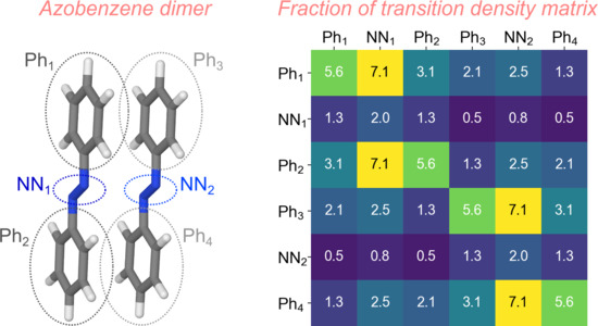
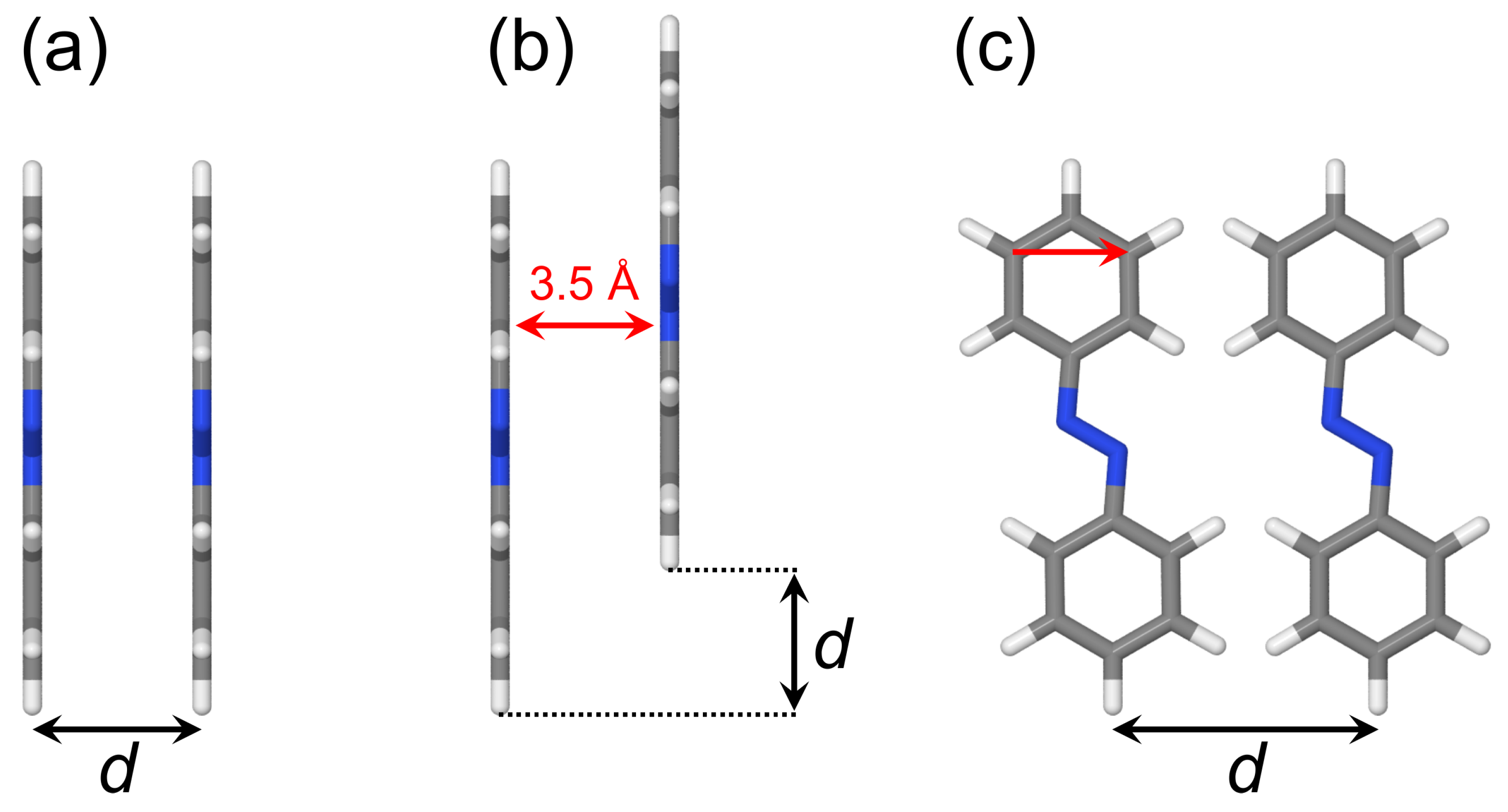
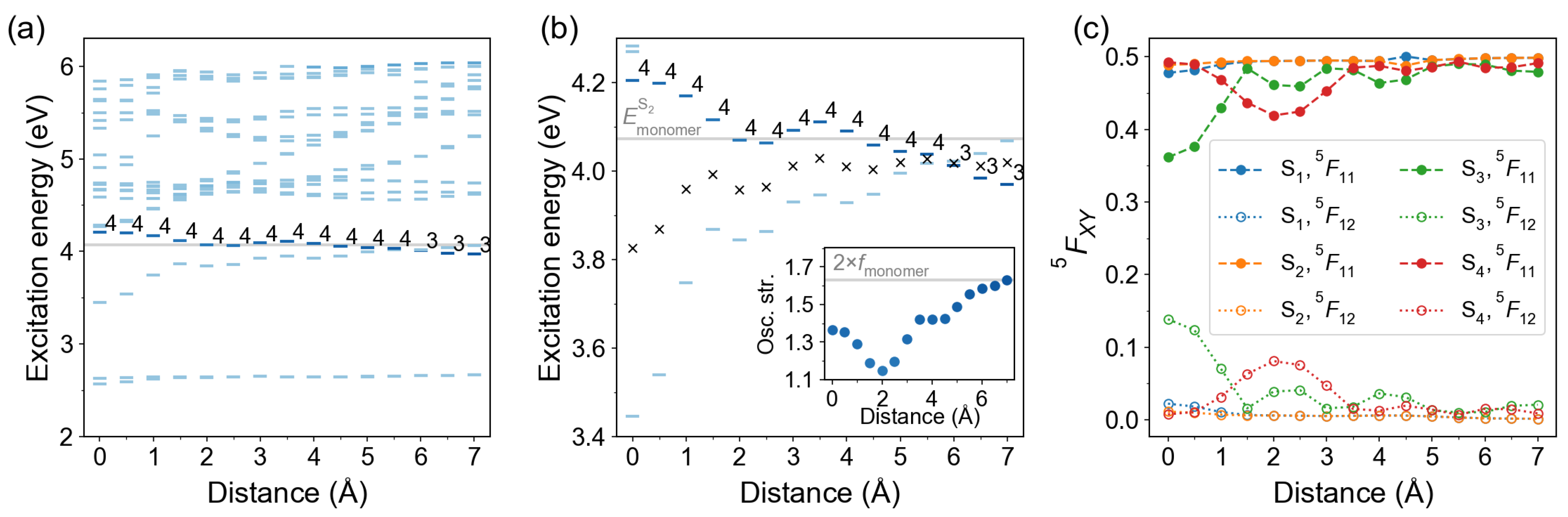
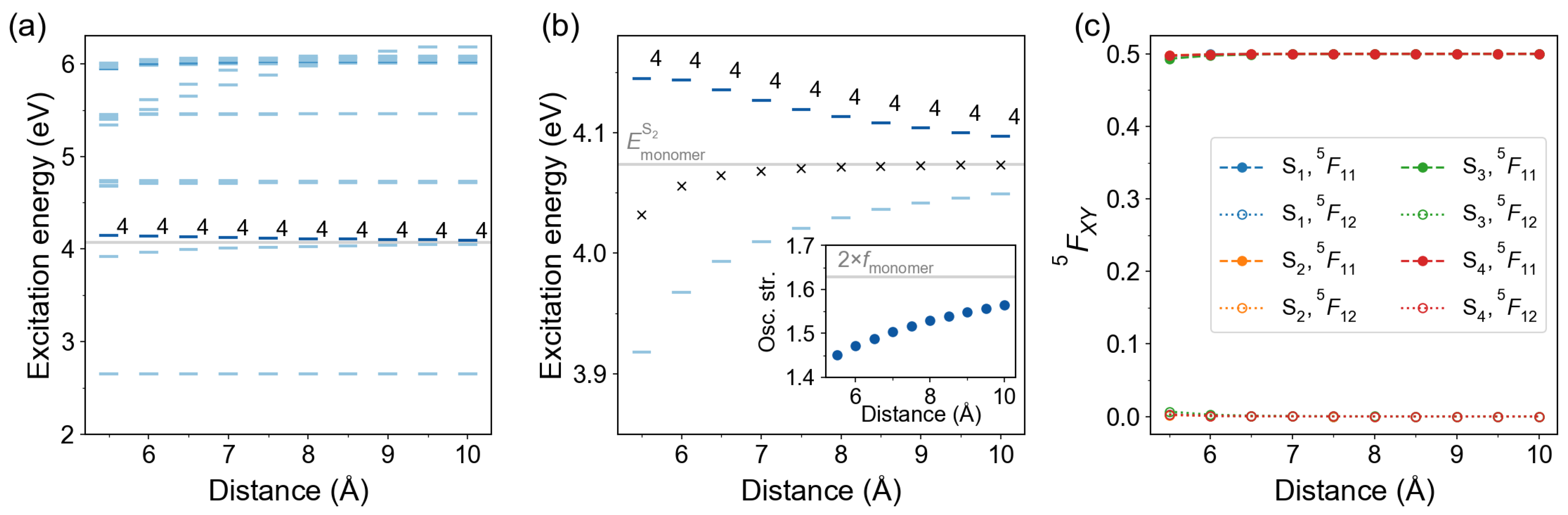
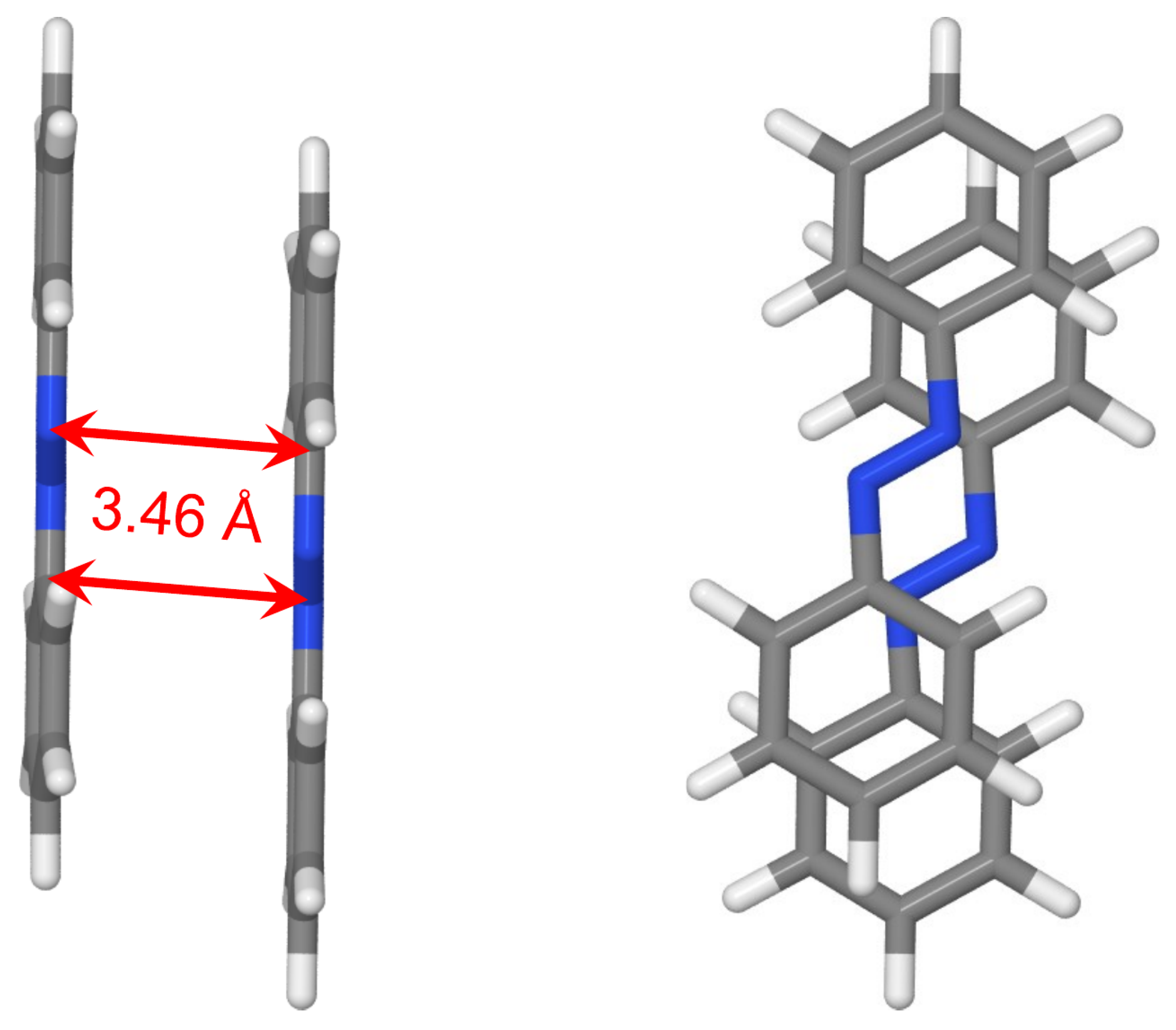
2.2.1. Cofacial -Stacked Dimer Å
2.2.2. Stacked Arrangement
2.2.3. Slip-Stacked Arrangement
2.2.4. In-Plane Arrangement
2.2.5. Optimized Dimer
3. Discussion
4. Materials and Methods
5. Conclusions
Supplementary Materials
Funding
Institutional Review Board Statement
Informed Consent Statement
Data Availability Statement
Acknowledgments
Conflicts of Interest
Sample Availability
Abbreviations
| TDM | Transition density matrix |
| FTDM | Fraction of transition density matrix |
| CT | Charge transfer |
| MO | Molecular orbital |
| AO | Atomic orbital |
| NTO | Natural transition orbital |
| DFT | Density functional theory |
| TD-DFT | Time-dependent density functional theory |
| ADC(2) | Algebraic diagrammatic construction through second order |
| CC2 | The second-order approximate coupled cluster singles and doubles model |
| CIS | Configuration interaction singles |
| HOMO | Highest occupied molecular orbital |
| LUMO | Lowest unoccupied molecular orbital |
| SI | Supporting Information |
Appendix A. TDM with Spin
References
- Goulet-Hanssens, A.; Eisenreich, F.; Hecht, S. Enlightening Materials with Photoswitches. Adv. Mater. 2020, 32, 1905966. [Google Scholar] [CrossRef] [PubMed]
- Bandara, H.M.D.; Burdette, S.C. Photoisomerization in different classes of azobenzene. Chem. Soc. Rev. 2012, 41, 1809–1825. [Google Scholar] [CrossRef] [PubMed]
- Gahl, C.; Schmidt, R.; Brete, D.; McNellis, E.R.; Freyer, W.; Carley, R.; Reuter, K.; Weinelt, M. Structure and Excitonic Coupling in Self-Assembled Monolayers of Azobenzene-Functionalized Alkanethiols. J. Am. Chem. Soc. 2010, 132, 1831–1838. [Google Scholar] [CrossRef] [PubMed]
- Utecht, M.; Klamroth, T.; Saalfrank, P. Optical absorption and excitonic coupling in azobenzenes forming self-assembled monolayers: A study based on density functional theory. Phys. Chem. Chem. Phys. 2011, 13, 21608–21614. [Google Scholar] [CrossRef] [PubMed]
- Zakrevskyy, Y.; Roxlau, J.; Brezesinski, G.; Lomadze, N.; Santer, S. Photosensitive surfactants: Micellization and interaction with DNA. J. Chem. Phys. 2014, 140, 044906. [Google Scholar] [CrossRef] [PubMed]
- Lund, R.; Brun, G.; Chevallier, E.; Narayanan, T.; Tribet, C. Kinetics of Photocontrollable Micelles: Light-Induced Self-Assembly and Disassembly of Azobenzene-Based Surfactants Revealed by TR-SAXS. Langmuir 2016, 32, 2539–2548. [Google Scholar] [CrossRef] [PubMed]
- Zakrevskyy, Y.; Titov, E.; Lomadze, N.; Santer, S. Phase diagrams of DNA-photosensitive surfactant complexes: Effect of ionic strength and surfactant structure. J. Chem. Phys. 2014, 141, 164904. [Google Scholar] [CrossRef]
- Kasyanenko, N.; Lysyakova, L.; Ramazanov, R.; Nesterenko, A.; Yaroshevich, I.; Titov, E.; Alexeev, G.; Lezov, A.; Unksov, I. Conformational and phase transitions in DNA-photosensitive surfactant solutions: Experiment and modeling. Biopolymers 2015, 103, 109–122. [Google Scholar] [CrossRef]
- Bléger, D.; Dokić, J.; Peters, M.V.; Grubert, L.; Saalfrank, P.; Hecht, S. Electronic Decoupling Approach to Quantitative Photoswitching in Linear Multiazobenzene Architectures. J. Phys. Chem. B 2011, 115, 9930–9940. [Google Scholar] [CrossRef]
- Zhao, F.; Grubert, L.; Hecht, S.; Bléger, D. Orthogonal switching in four-state azobenzene mixed-dimers. Chem. Commun. 2017, 53, 3323–3326. [Google Scholar] [CrossRef]
- Bahrenburg, J.; Sievers, C.M.; Schönborn, J.B.; Hartke, B.; Renth, F.; Temps, F.; Näther, C.; Sönnichsen, F.D. Photochemical properties of multi-azobenzene compounds. Photochem. Photobiol. Sci. 2013, 12, 511–518. [Google Scholar] [CrossRef] [PubMed]
- Lee, S.; Oh, S.; Lee, J.; Malpani, Y.; Jung, Y.S.; Kang, B.; Lee, J.Y.; Ozasa, K.; Isoshima, T.; Lee, S.Y.; et al. Stimulus-Responsive Azobenzene Supramolecules: Fibers, Gels, and Hollow Spheres. Langmuir 2013, 29, 5869–5877. [Google Scholar] [CrossRef]
- Koch, M.; Saphiannikova, M.; Santer, S.; Guskova, O. Photoisomers of Azobenzene Star with a Flat Core: Theoretical Insights into Multiple States from DFT and MD Perspective. J. Phys. Chem. B 2017, 121, 8854–8867. [Google Scholar] [CrossRef] [PubMed]
- Baroncini, M.; d’Agostino, S.; Bergamini, G.; Ceroni, P.; Comotti, A.; Sozzani, P.; Bassanetti, I.; Grepioni, F.; Hernandez, T.M.; Silvi, S.; et al. Photoinduced reversible switching of porosity in molecular crystals based on star-shaped azobenzene tetramers. Nat. Chem. 2015, 7, 634–640. [Google Scholar] [CrossRef] [PubMed]
- Slavov, C.; Yang, C.; Heindl, A.H.; Stauch, T.; Wegner, H.A.; Dreuw, A.; Wachtveitl, J. Twist and Return-Induced Ring Strain Triggers Quick Relaxation of a (Z)-Stabilized Cyclobisazobenzene. J. Phys. Chem. Lett. 2018, 9, 4776–4781. [Google Scholar] [CrossRef]
- Durgun, E.; Grossman, J.C. Photoswitchable Molecular Rings for Solar-Thermal Energy Storage. J. Phys. Chem. Lett. 2013, 4, 854–860. [Google Scholar] [CrossRef] [PubMed]
- Dong, L.; Feng, Y.; Wang, L.; Feng, W. Azobenzene-based solar thermal fuels: Design, properties, and applications. Chem. Soc. Rev. 2018, 47, 7339–7368. [Google Scholar] [CrossRef] [PubMed]
- Yang, C.; Slavov, C.; Wegner, H.A.; Wachtveitl, J.; Dreuw, A. Computational design of a molecular triple photoswitch for wavelength-selective control. Chem. Sci. 2018, 9, 8665–8672. [Google Scholar] [CrossRef] [PubMed]
- Kucharski, T.J.; Ferralis, N.; Kolpak, A.M.; Zheng, J.O.; Nocera, D.G.; Grossman, J.C. Templated assembly of photoswitches significantly increases the energy-storage capacity of solar thermal fuels. Nat. Chem. 2014, 6, 441. [Google Scholar] [CrossRef] [PubMed]
- Wang, Z.; Heinke, L.; Jelic, J.; Cakici, M.; Dommaschk, M.; Maurer, R.J.; Oberhofer, H.; Grosjean, S.; Herges, R.; Bräse, S.; et al. Photoswitching in nanoporous, crystalline solids: An experimental and theoretical study for azobenzene linkers incorporated in MOFs. Phys. Chem. Chem. Phys. 2015, 17, 14582–14587. [Google Scholar] [CrossRef]
- Davydov, A.S. The theory of molecular excitons. Sov. Phys. Uspekhi 1964, 7, 145–178. [Google Scholar] [CrossRef]
- Kasha, M.; Rawls, H.R.; El-Bayoumi, M.A. The exciton model in molecular spectroscopy. Pure Appl. Chem. 1965, 11, 371–392. [Google Scholar] [CrossRef]
- Hestand, N.J.; Spano, F.C. Expanded Theory of H- and J-Molecular Aggregates: The Effects of Vibronic Coupling and Intermolecular Charge Transfer. Chem. Rev. 2018, 118, 7069–7163. [Google Scholar] [CrossRef] [PubMed]
- Castillo, U.J.; Torres, A.E.; Fomine, S. Zinc-, cadmium-, and mercury-containing one-dimensional tetraphenylporphyrin arrays: A DFT study. J. Mol. Model. 2014, 20, 2206. [Google Scholar] [CrossRef] [PubMed]
- Li, D.; Titov, E.; Roedel, M.; Kolb, V.; Goetz, S.; Mitric, R.; Pflaum, J.; Brixner, T. Correlating Nanoscale Optical Coherence Length and Microscale Topography in Organic Materials by Coherent Two-Dimensional Microspectroscopy. Nano Lett. 2020, 20, 6452–6458. [Google Scholar] [CrossRef] [PubMed]
- Martin, R.L. Natural transition orbitals. J. Chem. Phys. 2003, 118, 4775–4777. [Google Scholar] [CrossRef]
- Luzanov, A.; Sukhorukov, A.; Umanskii, V. Application of transition density matrix for analysis of excited states. Theor. Exp. Chem. 1976, 10, 354–361. [Google Scholar] [CrossRef]
- Mayer, I. Using singular value decomposition for a compact presentation and improved interpretation of the CIS wave functions. Chem. Phys. Lett. 2007, 437, 284–286. [Google Scholar] [CrossRef]
- Titov, E.; Saalfrank, P. Exciton Splitting of Adsorbed and Free 4-Nitroazobenzene Dimers: A Quantum Chemical Study. J. Phys. Chem. A 2016, 120, 3055–3070. [Google Scholar] [CrossRef] [PubMed]
- Tretiak, S.; Mukamel, S. Density Matrix Analysis and Simulation of Electronic Excitations in Conjugated and Aggregated Molecules. Chem. Rev. 2002, 102, 3171–3212. [Google Scholar] [CrossRef]
- Plasser, F.; Lischka, H. Analysis of Excitonic and Charge Transfer Interactions from Quantum Chemical Calculations. J. Chem. Theory Comput. 2012, 8, 2777–2789. [Google Scholar] [CrossRef]
- McWeeny, R. Some Recent Advances in Density Matrix Theory. Rev. Mod. Phys. 1960, 32, 335–369. [Google Scholar] [CrossRef]
- Plasser, F.; Wormit, M.; Dreuw, A. New tools for the systematic analysis and visualization of electronic excitations. I. Formalism. J. Chem. Phys. 2014, 141, 024106. [Google Scholar] [CrossRef]
- Etienne, T. Transition matrices and orbitals from reduced density matrix theory. J. Chem. Phys. 2015, 142, 244103. [Google Scholar] [CrossRef]
- Furche, F. On the density matrix based approach to time-dependent density functional response theory. J. Chem. Phys. 2001, 114, 5982–5992. [Google Scholar] [CrossRef]
- Casida, M.E. Time-Dependent Density Functional Response Theory for Molecules. In Recent Advances in Density Functional Methods; Chong, D.P., Ed.; World Scientific: Singapore, 1995; pp. 155–192. [Google Scholar] [CrossRef]
- Mitrić, R.; Werner, U.; Bonačić-Koutecký, V. Nonadiabatic dynamics and simulation of time resolved photoelectron spectra within time-dependent density functional theory: Ultrafast photoswitching in benzylideneaniline. J. Chem. Phys. 2008, 129, 164118. [Google Scholar] [CrossRef] [PubMed]
- Du, L.; Lan, Z. Correction to An On-the-Fly Surface-Hopping Program JADE for Nonadiabatic Molecular Dynamics of Polyatomic Systems: Implementation and Applications. J. Chem. Theory Comput. 2015, 11, 4522–4523. [Google Scholar] [CrossRef] [PubMed]
- Crespo-Otero, R.; Barbatti, M. Recent Advances and Perspectives on Nonadiabatic Mixed Quantum–Classical Dynamics. Chem. Rev. 2018, 118, 7026–7068. [Google Scholar] [CrossRef] [PubMed]
- Nelson, T.; Fernandez-Alberti, S.; Roitberg, A.E.; Tretiak, S. Electronic Delocalization, Vibrational Dynamics, and Energy Transfer in Organic Chromophores. J. Phys. Chem. Lett. 2017, 8, 3020–3031. [Google Scholar] [CrossRef] [PubMed]
- Titov, E.; Humeniuk, A.; Mitrić, R. Exciton localization in excited-state dynamics of a tetracene trimer: A surface hopping LC-TDDFTB study. Phys. Chem. Chem. Phys. 2018, 20, 25995–26007. [Google Scholar] [CrossRef] [PubMed]
- Lu, T.; Chen, F. Multiwfn: A multifunctional wavefunction analyzer. J. Comput. Chem. 2012, 33, 580–592. [Google Scholar] [CrossRef] [PubMed]
- Luzanov, A.V.; Prezhdo, O.V. Irreducible charge density matrices for analysis of many-electron wave functions. Int. J. Quantum Chem. 2005, 102, 582–601. [Google Scholar] [CrossRef]
- Luzanov, A.V.; Zhikol, O.A. Electron invariants and excited state structural analysis for electronic transitions within CIS, RPA, and TDDFT models. Int. J. Quantum Chem. 2010, 110, 902–924. [Google Scholar] [CrossRef]
- Voityuk, A.A. Fragment transition density method to calculate electronic coupling for excitation energy transfer. J. Chem. Phys. 2014, 140, 244117. [Google Scholar] [CrossRef] [PubMed]
- Mai, S.; Plasser, F.; Dorn, J.; Fumanal, M.; Daniel, C.; González, L. Quantitative wave function analysis for excited states of transition metal complexes. Coord. Chem. Rev. 2018, 361, 74–97. [Google Scholar] [CrossRef]
- Plasser, F. TheoDORE: A toolbox for a detailed and automated analysis of electronic excited state computations. J. Chem. Phys. 2020, 152, 084108. [Google Scholar] [CrossRef]
- Fliegl, H.; Köhn, A.; Hättig, C.; Ahlrichs, R. Ab Initio Calculation of the Vibrational and Electronic Spectra of trans- and cis-Azobenzene. J. Am. Chem. Soc. 2003, 125, 9821–9827. [Google Scholar] [CrossRef]
- Cusati, T.; Granucci, G.; Martínez-Núñez, E.; Martini, F.; Persico, M.; Vázquez, S. Semiempirical Hamiltonian for Simulation of Azobenzene Photochemistry. J. Phys. Chem. A 2012, 116, 98–110. [Google Scholar] [CrossRef]
- Casellas, J.; Bearpark, M.J.; Reguero, M. Excited-State Decay in the Photoisomerisation of Azobenzene: A New Balance between Mechanisms. ChemPhysChem 2016, 17, 3068–3079. [Google Scholar] [CrossRef]
- Hutcheson, A.; Paul, A.C.; Myhre, R.H.; Koch, H.; Høyvik, I.M. Describing ground and excited state potential energy surfaces for molecular photoswitches using coupled cluster models. J. Comput. Chem. 2021, 42, 1419–1429. [Google Scholar] [CrossRef]
- Becke, A.D. Density-functional thermochemistry. III. The role of exact exchange. J. Chem. Phys. 1993, 98, 5648–5652. [Google Scholar] [CrossRef]
- Stephens, P.J.; Devlin, F.J.; Chabalowski, C.F.; Frisch, M.J. Ab Initio Calculation of Vibrational Absorption and Circular Dichroism Spectra Using Density Functional Force Fields. J. Phys. Chem. 1994, 98, 11623–11627. [Google Scholar] [CrossRef]
- Chai, J.D.; Head-Gordon, M. Long-range corrected hybrid density functionals with damped atom-atom dispersion corrections. Phys. Chem. Chem. Phys. 2008, 10, 6615–6620. [Google Scholar] [CrossRef] [PubMed]
- Schirmer, J. Beyond the random-phase approximation: A new approximation scheme for the polarization propagator. Phys. Rev. A 1982, 26, 2395–2416. [Google Scholar] [CrossRef]
- Trofimov, A.B.; Schirmer, J. An efficient polarization propagator approach to valence electron excitation spectra. J. Phys. B At. Mol. Opt. Phys. 1995, 28, 2299–2324. [Google Scholar] [CrossRef]
- Hättig, C. Structure Optimizations for Excited States with Correlated Second-Order Methods: CC2 and ADC(2). In Response Theory and Molecular Properties (A Tribute to Jan Linderberg and Poul Jørgensen); Jensen, H., Ed.; Academic Press: Cambridge, MA, USA, 2005; Volume 50, pp. 37–60. [Google Scholar] [CrossRef]
- Titov, E.; Hummert, J.; Ikonnikov, E.; Mitrić, R.; Kornilov, O. Electronic relaxation of aqueous aminoazobenzenes studied by time-resolved photoelectron spectroscopy and surface hopping TDDFT dynamics calculations. Faraday Discuss. 2021, 228, 226–241. [Google Scholar] [CrossRef]
- Ashfold, M.; Chergui, M.; Fischer, I.; Ge, L.; Grell, G.; Ivanov, M.; Kirrander, A.; Kornilov, O.; Krishnan, S.R.; Küpper, J.; et al. Time-resolved ultrafast spectroscopy: General discussion. Faraday Discuss. 2021, 228, 329–348. [Google Scholar] [CrossRef] [PubMed]
- Christiansen, O.; Koch, H.; Jørgensen, P. The second-order approximate coupled cluster singles and doubles model CC2. Chem. Phys. Lett. 1995, 243, 409–418. [Google Scholar] [CrossRef]
- Titov, E.; Granucci, G.; Götze, J.P.; Persico, M.; Saalfrank, P. Dynamics of Azobenzene Dimer Photoisomerization: Electronic and Steric Effects. J. Phys. Chem. Lett. 2016, 7, 3591–3596. [Google Scholar] [CrossRef] [PubMed]
- Hehre, W.J.; Ditchfield, R.; Pople, J.A. Self-Consistent Molecular Orbital Methods. XII. Further Extensions of Gaussian-Type Basis Sets for Use in Molecular Orbital Studies of Organic Molecules. J. Chem. Phys. 1972, 56, 2257–2261. [Google Scholar] [CrossRef]
- Hariharan, P.C.; Pople, J.A. The influence of polarization functions on molecular orbital hydrogenation energies. Theor. Chim. Acta 1973, 28, 213–222. [Google Scholar] [CrossRef]
- Weigend, F.; Ahlrichs, R. Balanced basis sets of split valence, triple zeta valence and quadruple zeta valence quality for H to Rn: Design and assessment of accuracy. Phys. Chem. Chem. Phys. 2005, 7, 3297–3305. [Google Scholar] [CrossRef] [PubMed]
- Dunning, T.H. Gaussian basis sets for use in correlated molecular calculations. I. The atoms boron through neon and hydrogen. J. Chem. Phys. 1989, 90, 1007–1023. [Google Scholar] [CrossRef]
- Kendall, R.A.; Dunning, T.H.; Harrison, R.J. Electron affinities of the first-row atoms revisited. Systematic basis sets and wave functions. J. Chem. Phys. 1992, 96, 6796–6806. [Google Scholar] [CrossRef]
- Dreuw, A.; Head-Gordon, M. Failure of Time-Dependent Density Functional Theory for Long-Range Charge-Transfer Excited States: The Zincbacteriochlorin–Bacteriochlorin and Bacteriochlorophyll–Spheroidene Complexes. J. Am. Chem. Soc. 2004, 126, 4007–4016. [Google Scholar] [CrossRef] [PubMed]
- Magyar, R.J.; Tretiak, S. Dependence of Spurious Charge-Transfer Excited States on Orbital Exchange in TDDFT: Large Molecules and Clusters. J. Chem. Theory Comput. 2007, 3, 976–987. [Google Scholar] [CrossRef] [PubMed]
- Liu, W.; Settels, V.; Harbach, P.H.P.; Dreuw, A.; Fink, R.F.; Engels, B. Assessment of TD-DFT- and TD-HF-based approaches for the prediction of exciton coupling parameters, potential energy curves, and electronic characters of electronically excited aggregates. J. Comput. Chem. 2011, 32, 1971–1981. [Google Scholar] [CrossRef]
- Hilborn, R.C. Einstein coefficients, cross sections, f values, dipole moments, and all that. Am. J. Phys. 1982, 50, 982–986. [Google Scholar] [CrossRef]
- Grimme, S.; Ehrlich, S.; Goerigk, L. Effect of the damping function in dispersion corrected density functional theory. J. Comput. Chem. 2011, 32, 1456–1465. [Google Scholar] [CrossRef]
- Carter-Fenk, K.; Herbert, J.M. Electrostatics does not dictate the slip-stacked arrangement of aromatic π–π interactions. Chem. Sci. 2020, 11, 6758–6765. [Google Scholar] [CrossRef]
- Hoffmann, M.; Schmidt, K.; Fritz, T.; Hasche, T.; Agranovich, V.; Leo, K. The lowest energy Frenkel and charge-transfer excitons in quasi-one-dimensional structures: Application to MePTCDI and PTCDA crystals. Chem. Phys. 2000, 258, 73–96. [Google Scholar] [CrossRef]
- East, A.L.L.; Lim, E.C. Naphthalene dimer: Electronic states, excimers, and triplet decay. J. Chem. Phys. 2000, 113, 8981–8994. [Google Scholar] [CrossRef]
- Shirai, S.; Iwata, S.; Tani, T.; Inagaki, S. Ab Initio Studies of Aromatic Excimers Using Multiconfiguration Quasi-Degenerate Perturbation Theory. J. Phys. Chem. A 2011, 115, 7687–7699. [Google Scholar] [CrossRef] [PubMed]
- Darghouth, A.A.M.H.M.; Correa, G.C.; Juillard, S.; Casida, M.E.; Humeniuk, A.; Mitrić, R. Davydov-type excitonic effects on the absorption spectra of parallel-stacked and herringbone aggregates of pentacene: Time-dependent density-functional theory and time-dependent density-functional tight binding. J. Chem. Phys. 2018, 149, 134111. [Google Scholar] [CrossRef] [PubMed]
- Fliegl, H.; You, Z.Q.; Hsu, C.P.; Sundholm, D. The Excitation Spectra of Naphthalene Dimers: Frenkel and Charge-transfer Excitons. J. Chin. Chem. Soc. 2016, 63, 20–32. [Google Scholar] [CrossRef]
- Darghouth, A.A.M.H.M.; Casida, M.E.; Zhu, X.; Natarajan, B.; Su, H.; Humeniuk, A.; Titov, E.; Miao, X.; Mitrić, R. Effect of varying the TD-lc-DFTB range-separation parameter on charge and energy transfer in a model pentacene/buckminsterfullerene heterojunction. J. Chem. Phys. 2021, 154, 054102. [Google Scholar] [CrossRef]
- Sánchez-Flores, E.I.; Chávez-Calvillo, R.; Keith, T.A.; Cuevas, G.; Rocha-Rinza, T.; Cortés-Guzmán, F. Properties of atoms in electronically excited molecules within the formalism of TDDFT. J. Comput. Chem. 2014, 35, 820–828. [Google Scholar] [CrossRef]
- Bader, R.F.W. Atoms in Molecules: A Quantum Theory; Oxford University Press: Oxford, UK, 1990. [Google Scholar]
- Frisch, M.J.; Trucks, G.W.; Schlegel, H.B.; Scuseria, G.E.; Robb, M.A.; Cheeseman, J.R.; Scalmani, G.; Barone, V.; Petersson, G.A.; Nakatsuji, H.; et al. Gaussian 16 Revision C.01; Gaussian Inc.: Wallingford, CT, USA, 2016. [Google Scholar]
- TURBOMOLE V7.0 2015, a Development of University of Karlsruhe and Forschungszentrum Karlsruhe GmbH, 1989–2007, TURBOMOLE GmbH, since 2007. Available online: http://www.turbomole.com (accessed on 18 June 2021).
- Balasubramani, S.G.; Chen, G.P.; Coriani, S.; Diedenhofen, M.; Frank, M.S.; Franzke, Y.J.; Furche, F.; Grotjahn, R.; Harding, M.E.; Hättig, C.; et al. TURBOMOLE: Modular program suite for ab initio quantum-chemical and condensed-matter simulations. J. Chem. Phys. 2020, 152, 184107. [Google Scholar] [CrossRef] [PubMed]
- Hättig, C.; Weigend, F. CC2 excitation energy calculations on large molecules using the resolution of the identity approximation. J. Chem. Phys. 2000, 113, 5154–5161. [Google Scholar] [CrossRef]
- Hättig, C.; Köhn, A. Transition moments and excited-state first-order properties in the coupled-cluster model CC2 using the resolution-of-the-identity approximation. J. Chem. Phys. 2002, 117, 6939–6951. [Google Scholar] [CrossRef]
- Hättig, C.; Hellweg, A.; Köhn, A. Distributed memory parallel implementation of energies and gradients for second-order Møller-Plesset perturbation theory with the resolution-of-the-identity approximation. Phys. Chem. Chem. Phys. 2006, 8, 1159–1169. [Google Scholar] [CrossRef] [PubMed]
- Weigend, F.; Häser, M.; Patzelt, H.; Ahlrichs, R. RI-MP2: Optimized auxiliary basis sets and demonstration of efficiency. Chem. Phys. Lett. 1998, 294, 143–152. [Google Scholar] [CrossRef]
- Weigend, F.; Köhn, A.; Hättig, C. Efficient use of the correlation consistent basis sets in resolution of the identity MP2 calculations. J. Chem. Phys. 2002, 116, 3175–3183. [Google Scholar] [CrossRef]
- Hättig, C. Optimization of auxiliary basis sets for RI-MP2 and RI-CC2 calculations: Core-valence and quintuple-ζ basis sets for H to Ar and QZVPP basis sets for Li to Kr. Phys. Chem. Chem. Phys. 2005, 7, 59–66. [Google Scholar] [CrossRef]


| TD-B3LYP | TD-B97X-D | |||||
|---|---|---|---|---|---|---|
| 6-31G* | def2-TZVP | aug-cc-pVTZ | 6-31G* | def2-TZVP | aug-cc-pVTZ | |
| B3LYP/def2-TZVP geometry | ||||||
| 2.52 (0.00) | 2.52 (0.00) | 2.52 (0.00) | 2.66 (0.00) | 2.66 (0.00) | 2.66 (0.00) | |
| 3.85 (0.78) | 3.74 (0.77) | 3.71 (0.76) | 4.19 (0.83) | 4.07 (0.81) | 4.05 (0.81) | |
| 4.18 (0.00) | 4.10 (0.05) | 4.09 (0.05) | 4.81 (0.03) | 4.71 (0.03) | 4.70 (0.03) | |
| 4.18 (0.05) | 4.10 (0.00) | 4.09 (0.00) | 4.82 (0.00) | 4.73 (0.00) | 4.71 (0.00) | |
| 4.90 (0.00) | 4.80 (0.00) | 4.77 (0.00) | 5.60 (0.00) | 5.46 (0.00) | 5.43 (0.00) | |
| B3LYP/6-31G* geometry | ||||||
| 2.55 (0.00) | 2.55 (0.00) | 2.55 (0.00) | 2.69 (0.00) | 2.68 (0.00) | 2.68 (0.00) | |
| 3.77 (0.77) | 3.66 (0.76) | 3.63 (0.76) | 4.10 (0.82) | 3.98 (0.80) | 3.96 (0.80) | |
| 4.11 (0.00) | 4.03 (0.05) | 4.01 (0.05) | 4.74 (0.03) | 4.64 (0.03) | 4.63 (0.03) | |
| 4.11 (0.05) | 4.03 (0.00) | 4.02 (0.00) | 4.75 (0.00) | 4.66 (0.00) | 4.64 (0.00) | |
| 4.83 (0.00) | 4.73 (0.00) | 4.70 (0.00) | 5.52 (0.00) | 5.38 (0.00) | 5.35 (0.00) | |
| ADC(2) | |||||
|---|---|---|---|---|---|
| aug-cc-pVDZ | aug-cc-pVTZ | aug-cc-pVQZ | def2-TZVP | def2-QZVP | |
| B3LYP/def2-TZVP geometry | |||||
| 2.81 (0.00) | 2.77 (0.00) | 2.77 (0.00) | 2.79 (0.00) | 2.77 (0.00) | |
| 4.19 (0.90) | 4.15 (0.89) | 4.14 (0.89) | 4.20 (0.91) | 4.15 (0.90) | |
| 4.58 (0.03) | 4.53 (0.03) | 4.52 (0.03) | 4.57 (0.03) | 4.53 (0.03) | |
| 4.59 (0.00) | 4.54 (0.00) | 4.53 (0.00) | 4.57 (0.00) | 4.54 (0.00) | |
| 5.32 (0.00) | 5.27 (0.00) | 5.26 (0.00) | 5.33 (0.00) | 5.28 (0.00) | |
| B3LYP/6-31G* geometry | |||||
| 2.84 (0.00) | 2.80 (0.00) | 2.80 (0.00) | 2.82 (0.00) | 2.80 (0.00) | |
| 4.10 (0.89) | 4.06 (0.89) | 4.05 (0.89) | 4.11 (0.90) | 4.06 (0.89) | |
| 4.51 (0.03) | 4.46 (0.03) | 4.44 (0.03) | 4.49 (0.03) | 4.45 (0.03) | |
| 4.52 (0.00) | 4.46 (0.00) | 4.45 (0.00) | 4.50 (0.00) | 4.46 (0.00) | |
| 5.24 (0.00) | 5.18 (0.00) | 5.17 (0.00) | 5.24 (0.00) | 5.19 (0.00) | |
| TD-B3LYP/def2-TZVP | TD-B97X-D/def2-TZVP | ADC(2)/aug-cc-pVTZ | |
|---|---|---|---|
| 2.36 (0.00) | 2.57 (0.00) | 2.65 (0.00) | |
| 2.46 (0.00) | 2.63 (0.00) | 2.72 (0.00) | |
| 2.82 (0.00) | 3.45 (0.00) | 3.46 (0.00) | |
| 3.28 (0.00) | 4.21 (1.37) | 4.04 (0.00) | |
| 3.37 (0.00) | 4.27 (0.00) | 4.04 (0.00) | |
| 3.40 (0.00) | 4.28 (0.00) | 4.20 (1.50) | |
| 3.45 (0.00) | 4.59 (0.00) | 4.47 (0.04) | |
| 3.46 (0.00) | 4.66 (0.00) | 4.48 (0.00) | |
| 3.88 (1.24) | 4.67 (0.00) | 4.51 (0.00) | |
| 4.06 (0.00) | 4.73 (0.04) | 4.56 (0.00) |
| TD-B3LYP/def2-TZVP | TD-B97X-D/def2-TZVP | ADC(2)/aug-cc-pVTZ | |
|---|---|---|---|
| 2.51 (0.00) | 2.65 (0.00) | 2.74 (0.00) | |
| 2.52 (0.00) | 2.65 (0.00) | 2.74 (0.00) | |
| 3.23 (0.02) | 3.85 (0.00) | 3.91 (0.00) | |
| 3.23 (0.00) | 4.10 (1.15) | 4.09 (1.24) | |
| 3.37 (0.05) | 4.52 (0.00) | 4.36 (0.00) | |
| 3.38 (0.00) | 4.56 (0.13) | 4.37 (0.01) | |
| 3.50 (0.00) | 4.60 (0.00) | 4.42 (0.02) | |
| 3.82 (0.13) | 4.61 (0.01) | 4.42 (0.00) | |
| 3.84 (0.00) | 4.67 (0.08) | 4.45 (0.00) | |
| 3.84 (0.82) | 4.70 (0.00) | 4.47 (0.15) |
Publisher’s Note: MDPI stays neutral with regard to jurisdictional claims in published maps and institutional affiliations. |
© 2021 by the author. Licensee MDPI, Basel, Switzerland. This article is an open access article distributed under the terms and conditions of the Creative Commons Attribution (CC BY) license (https://creativecommons.org/licenses/by/4.0/).
Share and Cite
Titov, E. On the Low-Lying Electronically Excited States of Azobenzene Dimers: Transition Density Matrix Analysis. Molecules 2021, 26, 4245. https://doi.org/10.3390/molecules26144245
Titov E. On the Low-Lying Electronically Excited States of Azobenzene Dimers: Transition Density Matrix Analysis. Molecules. 2021; 26(14):4245. https://doi.org/10.3390/molecules26144245
Chicago/Turabian StyleTitov, Evgenii. 2021. "On the Low-Lying Electronically Excited States of Azobenzene Dimers: Transition Density Matrix Analysis" Molecules 26, no. 14: 4245. https://doi.org/10.3390/molecules26144245
APA StyleTitov, E. (2021). On the Low-Lying Electronically Excited States of Azobenzene Dimers: Transition Density Matrix Analysis. Molecules, 26(14), 4245. https://doi.org/10.3390/molecules26144245