Discrimination of Gentiana and Its Related Species Using IR Spectroscopy Combined with Feature Selection and Stacked Generalization

Abstract

Gentiana, which is one of the largest genera of Gentianoideae, most of which had potential pharmaceutical value, and applied to local traditional medical treatment. Because of the phytochemical diversity and difference of bioactive compounds among species, which makes it crucial to accurately identify authentic Gentiana species. In this paper, the feasibility of using the infrared spectroscopy technique combined with chemometrics analysis to identify Gentiana and its related species was studied. A total of 180 batches of raw spectral fingerprints were obtained from 18 species of Gentiana and Tripterospermum by near-infrared (NIR: 10,000–4000 cm⁻¹) and Fourier transform mid-infrared (MIR: 4000–600 cm⁻¹) spectrum. Firstly, principal component analysis (PCA) was utilized to explore the natural grouping of the 180 samples. Secondly, random forests (RF), support vector machine (SVM), and K-nearest neighbors (KNN) models were built while using full spectra (including 1487 NIR variables and 1214 FT-MIR variables, respectively). The MIR-SVM model had a higher classification accuracy rate than the other models that were based on the results of the calibration sets and prediction sets. The five feature selection strategies, VIP (variable importance in the projection), Boruta, GARF (genetic algorithm combined with random forest), GASVM (genetic algorithm combined with support vector machine), and Venn diagram calculation, were used to reduce the dimensions of the data variable in order to further reduce numbers of variables for modeling. Finally, 101 NIR and 73 FT-MIR bands were selected as the feature variables, respectively. Thirdly, stacking models were built based on the optimal spectral dataset. Most of the stacking models performed better than the full spectra-based models. RF and SVM (as base learners), combined with the SVM meta-classifier, was the optimal stacked generalization strategy. For the SG-Ven-MIR-SVM model, the accuracy (ACC) of the calibration set and validation set were both 100%. Sensitivity (SE), specificity (SP), efficiency (EFF), Matthews correlation coefficient (MCC), and Cohen’s kappa coefficient (K) were all 1, which showed that the model had the optimal authenticity identification performance. Those parameters indicated that stacked generalization combined with feature selection is probably an important technique for improving the classification model predictive accuracy and avoid overfitting. The study result can provide a valuable reference for the safety and effectiveness of the clinical application of medicinal Gentiana.

1. Introduction

Genus Gentiana is one of the largest groups in Gentianaceae, comprising 360 species that are widespread across Northwest of Africa, Europe, America, East of Australia, and Asia [1]. Many species of this genus have significant economic value and they are widely used by the food and pharmaceutical industries in the world [2,3,4]. In Europe, G. lutea (Yellow Gentian) are traditional materials for alcoholic bitter beverages and have a function of being appetite stimulating and improving digestion [4,5]. In Asia, Gentiana has a long history in use for medicine [2,3,6]. Places, including Iran, Mongolia, Japan and Korea have literature and details about nature and the of medicinal Gentiana plants found in these countries [3,7,8]. In China, species of Gentiana are diverse (about 248 species) and some of them have been an important part of traditional Chinese medicine (TCM) for a long time [1,9]. Approximattely 2000 years ago, Chinese Medicine monographs, “Shen Nong Ben Cao Jing”, had described and recorded function and medicinal value of Longdan (Gentianae Radix et Rhizoma: dried root and rhizome of G rigescens, G. trifloral, G. manshurica and G. scabra) and Qinjiao (Gentianae Macrophyllae Radix: dried root of G. macrophylla, G. straminea, G. crassicaulis, and G. dahurica) [10]. Presently, nine species of Gentiana have been recorded as the official drug of Pharmacopoeia of the People’s Republic of China (Ch.P. 2015 edition) [9]. But besides that, G. cephalantha, G. davidii, G. loureirii, G. rubicunda G, lawrencei var. farreri, and other species have been used as a popular herb in folk medicine and many other ethnomedicines for remedy digestive and respiratory illnesses [11,12,13]. Gentiana and its related species are extensively used for various health disorders due to the cheap price of traditional herbs [13]. These medicinal plants have always played an important role in the health care of local people, especially in the underdeveloped area of southwest China.

Chemical and pharmacological researches have indicated that the composition of bioactive compounds is diverse according to different Gentiana species [2,6]. Until now, more than 500 secondary metabolites have been isolated from approximately 60 species [2]. Those compounds, including iridoids, triterpenoids, flavonoids, alkaloids, and other types of secondary metabolites [2,14,15]. Gentiana species have different therapeutic properties and medicinal functions because of the complicated chemical profiles [2,13,14]. For example, G. lute and G. rigescens could be used as raw materials for the preparation of the therapeutic drug for Alzheimer’s disease because of neuritogenic compounds that were isolated from the two species [4,16,17]. Although G. straminea and G. scabra are rich in iridoids, chemical composition and traditional uses are different between the two species. G. straminea is used for treating rheumatic arthritis, while G. scabra is used for liver protection [6,14]. G. rhodantha and G. rigescens usually are often confused in traditional medicine markets in southwest China. In fact, the former is good at treating cough and other throat illnesses that are caused by fever, and, while the latter is used for chronic liver disease, inflammatory skin diseases, and clearing away heat [9,13]. Those cases showed that the identification of Gentiana species is crucial for keeping the clinical effect consistent and ensuring patients’ medication safety.

Gentiana species show extremely high morphological similarity and their Chinese names of species are often used in confusion in the market (see sample information). Furthermore, the powder of medicinal materials of Gentiana species is difficult for achieving the identification. Although pharmacognosy morphology identification or microscopic identification based on inner structural composition features and the inclusions of medicinal materials may be used for this purpose [9]; these works critically depend on personal experiences. In recent years, the researches regarding authenticity identification and discrimination of Gentiana and its relatives were focused on DNA barcoding, ISSR amplification, and other molecular identification technologies [18,19,20,21]. In addition, chromatographic and mass-spectrometric techniques were applied for species classification [10,22,23]. However, these methods need a complex process of extractions, tedious pretreatment, a great number of chemical reagents, waste time, and are expensive. A rapid, high-accurate, and green authenticity identification method needs to be established to ensure the effectiveness and safety of the clinical application of Gentiana. In the past few decades, ultraviolet-visible (UV-Vis), Raman, and infrared (IR) spectroscopic have gained the attention of various botany scientists and pharmacognosists [23,24,25,26]. Among them, near-infrared (NIR) and mid-infrared (MIR) spectroscopy are probably the most publicized technologies [27,28,29,30]. These two technologies can provide detailed structural information on sample properties and composition at the molecular level [31,32,33,34]. Like human fingerprints, the infrared spectrum of any substance has to be unique [31]. This is the reason for NIR and MIR spectral fingerprints can be applied to identify or classify different samples [31,32,33,34]. In the case of medicinal plants, chemical constituents and their ratios of biochemicals of different species can vary substantially [35,36]. The IR spectroscopy could be used for the identification of medicinal species because the corresponding spectral signals of these chemicals are highly specific [35,36]. Recently, successful species discrimination of Dendrobium, Paris, Rhodiola, Ganoderma, and the other genus based on IR spectroscopy has been reported [35,36,37,38].

In the process of spectral discrimination, it is necessary to establish a relationship between the chemical information and sample categories by chemometrics then to establish a classification model for the class identification of unknown samples [39]. Additionally, feature variable selection and model optimization strategy that are based on chemometrics are key steps during the model building [40]. From the literature, it can be found that a combination of variable selection methods and different algorithms could provide multifarious modeling strategies and most of them showed the superior ability for classification and identification [41,42]. With the development of modeling methods, Wolpert developed stacked generalization in the early 1990s [43]. This method combines multiple models together to produce a meta-model with equal or better classification performance than the constituent parts [43,44]. In theory, this modeling strategy belongs to the ensemble model, and its classification result might be better than any of the constituent sub-models [44,45]. For example, Shan’s research showed that the performance of an extreme learning machine model that was based on stacked generalization was more robust than the traditional model [46]. Sfakianakis’s research reported a similar finding [47]. Although stacked generalization might be an approach for improving model prediction accuracy and robustness, there was limited reporting of this method applied to medicinal plant research.

The aim of this research was (1) to investigate the application of NIR (near-infrared) and FT-MIR (Fourier transform mid-infrared) spectroscopies to the classification of medicinal Gentiana and its wild relatives; (2) to select the optimal bands that identify the differences among different species; and, (3) to examine the feasibility of using stacked generalization combined with infrared spectral data to identify Gentiana species. The results of the study may provide some basis for the safety and effectiveness utilization of medicinal Gentiana resources in China.

2. Results and Discussion

2.1. Spectral Fingerprint of NIR and FT-MIR

Figure 1 shows the raw NIR spectra and FT-MIR that were obtained from 180 samples of G. rigescens and their relatives. It can be seen from the raw NIR spectra that there are seven distinct absorption bands, which are located at 6920, 5781, 5669, 5174, 4761, 4331, and 4260 cm⁻¹, respectively (Figure 1A). In the whole FT-MIR spectral range (Figure 1B), 3335, 2924, 2853, 1735, 1636, 1516, 1319, 1265, 1147, 1033, and 831 cm⁻¹ appeared in all species.

In the range of 7171–6514 cm⁻¹, G. rhodantha is clearly different from the other two traditional medicinal Gentiana species. It is interesting that the NIR spectra of T. chinense and T. cordatum are similar to G. rigescens and G. crassicaulis. The spectral intensity of G. davidii at 4225 cm⁻¹ was different from G. rigescens and G. cephalantha (Figure 2). In fact, the three species have similar plant morphology and G. cephalantha and G. davidii are primary alternative species of G. rigescens in remote rural of the southwest of China.

The FT-MIR spectra of 18 species showed very similar band distributions in the whole spectral range of 3587–2827 cm⁻¹, but there were differences in the relative intensities of the spectral absorption bands of samples in the range of 1780–600 cm⁻¹ (Figure 3). For example, the huge spectral differences between the bands 1709–1531, 1478–1207, 1168–1130, 1114–1015, 948–883, and 822–740 cm⁻¹ were observed among G. rigescens, G. crassicaulis, G. rhodantha, G. davidii, G. pseudosquarrosa, and G. stragulata. Obviously, the fingerprints of Tripterospermum species and Gentiana species were significantly different in the 1650–1600, 1579–1494, 1458–1393, 1164–1126, 1112–1090, 950–883, and 822–740 cm⁻¹, respectively (Figure 3).

2.2. Exploratory Statistical Analysis

Before statistical analysis, all of the spectra datasets were pretreated by the second derivative and standard normal variate for improving visualization results. The score plots that were obtained after principal component analysis (PCA) on the NIR data set are shown in Figure 4. A faint clustering of samples was observed in the figure. The score-plot for PC1 vs. PC2 displays G. squarrosa (11) could be clearly separated from other species (Figure 4A). In Score-plot for PC1 vs. PC3, G stragulata (5) and T. cordatum (18) were clustered and samples from the G. crassicaulis (6) were more easily differentiated from other samples (Figure 4B).

Figure 5 shows score plots that were obtained by an application of PCA on the FT-MIR spectra data. According to the scatter plot of PC1 vs. PC2, G. stragulata (5) and G. pseudosquarrosa (12) were clustered. The samples of G. lawrencei var. farreri (4), G. rhodantha (15), and G. striata (16) were both located in the middle of the PC1 and PC2 axes. Most of the samples of G. squarrosa (11) were significantly different from other species and they were located on the negative side of PC1 and PC2. With the exception of the above species, all of the other species are grouped into one group (Figure 5A). From the scatter plot of PC1 vs. PC3. G. stragulata (5) and G. crassicaulis (6) were each separately clustered. Additionally, samples from the G. squarrosa (11) could be distinguished from those of the G. pseudosquarrosa (12) (Figure 5B).

The grouping results indicated a potential application value of NIR and FT-MIR fingerprint for the discrimination of medicinal Gentiana and its related species. Nonetheless, most of Gentiana species would be difficult to differentiate from one another, due to the overlap of their sample score. Hence, the application of supervised pattern recognition methods, such as random forest (RF), support vector machines (SVM), and k-nearest neighbors (KNN), for the development of classification models were required for enabling one to distinguish the samples.

2.3. Single Block Models for Sample Classification

2.3.1. Classification Based on Full Spectra

In the section, all of the classification models were established by full spectra data (the total number of points in NIR and FT-MIR is 1487 and 1214, respectively) and 180 samples were separated into a calibration set (108 samples) and a validation set (72 samples) by the Kennard–Stone algorithm [48]. Six performance parameters, including sensitivity (SE), specificity (SP), efficiency (EFF), accuracy (ACC), Matthews correlation coefficient (MCC), and Cohen’s kappa coefficient (K), were applied to evaluate the identification ability of classification models [49,50]. Those parameters values range from 0 to 1, indicating a perfect classification when the values are 1 [49].

For RF models, model performance depends on the proper selection of the hyperparameters, which are n_tree and m_try [49]. Figures S1 and S2 show the suitable hyperparameters and variation of model mean misclassification error (MMCE) with different hyperparameters. The lower MMCE the hyperparameter was better [50].

Table 1. The major parameters of random forests (RF) model based on NIR full spectra data.

Class	Calibration Set					Validation Set
	ACC (%)	SE	SP	MCC	EFF	ACC (%)	SE	SP	MCC	EFF
1	100.00	1.00	1.00	1.00	1.00	100.00	1.00	1.00	1.00	1.00
2	100.00	1.00	1.00	1.00	1.00	100.00	1.00	1.00	1.00	1.00
3	100.00	1.00	1.00	1.00	1.00	100.00	1.00	1.00	1.00	1.00
4	100.00	1.00	1.00	1.00	1.00	100.00	1.00	1.00	1.00	1.00
5	100.00	1.00	1.00	1.00	1.00	97.22	0.75	0.99	0.74	0.86
6	100.00	1.00	1.00	1.00	1.00	100.00	1.00	1.00	1.00	1.00
7	100.00	1.00	1.00	1.00	1.00	100.00	1.00	1.00	1.00	1.00
8	100.00	1.00	1.00	1.00	1.00	98.61	0.75	1.00	0.86	0.87
9	100.00	1.00	1.00	1.00	1.00	98.61	1.00	0.99	0.89	0.99
10	100.00	1.00	1.00	1.00	1.00	100.00	1.00	1.00	1.00	1.00
11	100.00	1.00	1.00	1.00	1.00	100.00	1.00	1.00	1.00	1.00
12	100.00	1.00	1.00	1.00	1.00	97.22	0.75	0.99	0.74	0.86
13	100.00	1.00	1.00	1.00	1.00	100.00	1.00	1.00	1.00	1.00
14	100.00	1.00	1.00	1.00	1.00	100.00	1.00	1.00	1.00	1.00
15	100.00	1.00	1.00	1.00	1.00	100.00	1.00	1.00	1.00	1.00
16	100.00	1.00	1.00	1.00	1.00	97.22	0.75	0.99	0.74	0.86
17	100.00	1.00	1.00	1.00	1.00	100.00	1.00	1.00	1.00	1.00
18	100.00	1.00	1.00	1.00	1.00	97.22	0.75	0.99	0.74	0.86

and

Table 2. The major parameters of RF model based on FT-MIR full spectra data.

Class	Calibration Set					Validation Set
	ACC (%)	SE	SP	MCC	EFF	ACC (%)	SE	SP	MCC	EFF
1	100.00	1.00	1.00	1.00	1.00	100.00	1.00	1.00	1.00	1.00
2	100.00	1.00	1.00	1.00	1.00	100.00	1.00	1.00	1.00	1.00
3	100.00	1.00	1.00	1.00	1.00	100.00	1.00	1.00	1.00	1.00
4	100.00	1.00	1.00	1.00	1.00	100.00	1.00	1.00	1.00	1.00
5	100.00	1.00	1.00	1.00	1.00	100.00	1.00	1.00	1.00	1.00
6	100.00	1.00	1.00	1.00	1.00	100.00	1.00	1.00	1.00	1.00
7	100.00	1.00	1.00	1.00	1.00	100.00	1.00	1.00	1.00	1.00
8	100.00	1.00	1.00	1.00	1.00	98.61	0.75	1.00	0.86	0.87
9	100.00	1.00	1.00	1.00	1.00	98.61	1.00	0.99	0.89	0.99
10	100.00	1.00	1.00	1.00	1.00	98.61	1.00	0.99	0.89	0.99
11	100.00	1.00	1.00	1.00	1.00	98.61	1.00	0.99	0.89	0.99
12	100.00	1.00	1.00	1.00	1.00	98.61	0.75	1.00	0.86	0.87
13	100.00	1.00	1.00	1.00	1.00	100.00	1.00	1.00	1.00	1.00
14	100.00	1.00	1.00	1.00	1.00	100.00	1.00	1.00	1.00	1.00
15	100.00	1.00	1.00	1.00	1.00	98.61	1.00	0.99	0.89	0.99
16	100.00	1.00	1.00	1.00	1.00	97.22	0.50	1.00	0.70	0.71
17	100.00	1.00	1.00	1.00	1.00	100.00	1.00	1.00	1.00	1.00
18	100.00	1.00	1.00	1.00	1.00	100.00	1.00	1.00	1.00	1.00

present classification accuracies rates in the calibration and validation data sets of 18 species that were obtained by NIR-RF and FT-MIR-RF models. For the two models, all of the samples in the calibration set were correctly classified. Additionally, the accuracy rates of validation sets were not less than 97.22%. Although the FT-MIR-RF model had higher total validation accuracy (94.44%), its SE, MCC, and EFF values of the validation set were lower than the NIR-RF model. Hence, the phenomenon of imbalance category recognition in the FT-MIR-RF model was worse (Table 1 and Table 2).

For the SVM models, the optimum kernel function (sigmoid, polynomial, and radial kernel) and the cost function were important for modeling [35,51]. Hyperparameter optimization results showed the linear kernel had lower MMCE value than sigmoid, polynomial, and radial kernel. Hence, the linear kernel was suitable for modeling (Figures S3 and S4). Subsequently, the cost function was optimized. And the most suitable values 5 and 0.05 were selected as the best cost function for the SVM models of NIR and FT-MIR, respectively (Figures S3 and S4).

Table 3. The major parameters of SVM model based on NIR full spectra data.

Class	Calibration Set					Validation Set
	ACC (%)	SE	SP	MCC	EFF	ACC (%)	SE	SP	MCC	EFF
1	100.00	1.00	1.00	1.00	1.00	98.61	0.75	1.00	0.86	0.87
2	100.00	1.00	1.00	1.00	1.00	100.00	1.00	1.00	1.00	1.00
3	100.00	1.00	1.00	1.00	1.00	100.00	1.00	1.00	1.00	1.00
4	100.00	1.00	1.00	1.00	1.00	100.00	1.00	1.00	1.00	1.00
5	100.00	1.00	1.00	1.00	1.00	97.22	0.75	0.99	0.74	0.86
6	100.00	1.00	1.00	1.00	1.00	100.00	1.00	1.00	1.00	1.00
7	100.00	1.00	1.00	1.00	1.00	98.61	1.00	0.99	0.89	0.99
8	100.00	1.00	1.00	1.00	1.00	98.61	0.75	1.00	0.86	0.87
9	100.00	1.00	1.00	1.00	1.00	98.61	1.00	0.99	0.89	0.99
10	100.00	1.00	1.00	1.00	1.00	100.00	1.00	1.00	1.00	1.00
11	100.00	1.00	1.00	1.00	1.00	100.00	1.00	1.00	1.00	1.00
12	100.00	1.00	1.00	1.00	1.00	97.22	0.75	0.99	0.74	0.86
13	100.00	1.00	1.00	1.00	1.00	100.00	1.00	1.00	1.00	1.00
14	100.00	1.00	1.00	1.00	1.00	100.00	1.00	1.00	1.00	1.00
15	100.00	1.00	1.00	1.00	1.00	100.00	1.00	1.00	1.00	1.00
16	100.00	1.00	1.00	1.00	1.00	97.22	0.75	0.99	0.74	0.86
17	100.00	1.00	1.00	1.00	1.00	100.00	1.00	1.00	1.00	1.00
18	100.00	1.00	1.00	1.00	1.00	97.22	0.75	0.99	0.74	0.86

and

Table 4. The major parameters of SVM model based on FT-MIR full spectra data.

Class	Calibration Set					Validation Set
	ACC (%)	SE	SP	MCC	EFF	ACC (%)	SE	SP	MCC	EFF
1	100.00	1.00	1.00	1.00	1.00	100.00	1.00	1.00	1.00	1.00
2	100.00	1.00	1.00	1.00	1.00	100.00	1.00	1.00	1.00	1.00
3	100.00	1.00	1.00	1.00	1.00	100.00	1.00	1.00	1.00	1.00
4	100.00	1.00	1.00	1.00	1.00	100.00	1.00	1.00	1.00	1.00
5	100.00	1.00	1.00	1.00	1.00	100.00	1.00	1.00	1.00	1.00
6	100.00	1.00	1.00	1.00	1.00	100.00	1.00	1.00	1.00	1.00
7	100.00	1.00	1.00	1.00	1.00	100.00	1.00	1.00	1.00	1.00
8	100.00	1.00	1.00	1.00	1.00	100.00	1.00	1.00	1.00	1.00
9	100.00	1.00	1.00	1.00	1.00	100.00	1.00	1.00	1.00	1.00
10	100.00	1.00	1.00	1.00	1.00	100.00	1.00	1.00	1.00	1.00
11	100.00	1.00	1.00	1.00	1.00	100.00	1.00	1.00	1.00	1.00
12	100.00	1.00	1.00	1.00	1.00	100.00	1.00	1.00	1.00	1.00
13	100.00	1.00	1.00	1.00	1.00	100.00	1.00	1.00	1.00	1.00
14	100.00	1.00	1.00	1.00	1.00	100.00	1.00	1.00	1.00	1.00
15	100.00	1.00	1.00	1.00	1.00	100.00	1.00	1.00	1.00	1.00
16	100.00	1.00	1.00	1.00	1.00	100.00	1.00	1.00	1.00	1.00
17	100.00	1.00	1.00	1.00	1.00	100.00	1.00	1.00	1.00	1.00
18	100.00	1.00	1.00	1.00	1.00	100.00	1.00	1.00	1.00	1.00

present the major parameters of the calibration and validation sets for NIR-SVM and FT-MIR-SVM models. It could be seen that the samples of 18 species were better discriminated by using the FT-MIR data set. FT-MIR-SVM model achieved 100% total accuracy for the calibration set and validation sets.

Determining parameter k is critical for KNN [52]. Hence, this hyperparameter was optimized before modeling and the optimum k value for NIR and FT-MIR data set were both one (Figures S5 and S6).

Table 5. The major parameters of K-nearest neighbors (KNN) model based on NIR full spectra data.

Class	Calibration Set					Validation Set
	ACC (%)	SE	SP	MCC	EFF	ACC (%)	SE	SP	MCC	EFF
1	100.00	1.00	1.00	1.00	1.00	98.61	1.00	0.99	0.89	0.99
2	100.00	1.00	1.00	1.00	1.00	97.22	0.50	1.00	0.70	0.71
3	100.00	1.00	1.00	1.00	1.00	100.00	1.00	1.00	1.00	1.00
4	100.00	1.00	1.00	1.00	1.00	100.00	1.00	1.00	1.00	1.00
5	100.00	1.00	1.00	1.00	1.00	95.83	0.75	0.97	0.65	0.85
6	100.00	1.00	1.00	1.00	1.00	100.00	1.00	1.00	1.00	1.00
7	100.00	1.00	1.00	1.00	1.00	98.61	0.75	1.00	0.86	0.87
8	100.00	1.00	1.00	1.00	1.00	100.00	1.00	1.00	1.00	1.00
9	100.00	1.00	1.00	1.00	1.00	97.22	0.75	0.99	0.74	0.86
10	100.00	1.00	1.00	1.00	1.00	100.00	1.00	1.00	1.00	1.00
11	100.00	1.00	1.00	1.00	1.00	100.00	1.00	1.00	1.00	1.00
12	100.00	1.00	1.00	1.00	1.00	95.83	0.75	0.97	0.65	0.85
13	100.00	1.00	1.00	1.00	1.00	100.00	1.00	1.00	1.00	1.00
14	100.00	1.00	1.00	1.00	1.00	100.00	1.00	1.00	1.00	1.00
15	100.00	1.00	1.00	1.00	1.00	100.00	1.00	1.00	1.00	1.00
16	100.00	1.00	1.00	1.00	1.00	97.22	0.75	0.99	0.74	0.86
17	100.00	1.00	1.00	1.00	1.00	100.00	1.00	1.00	1.00	1.00
18	100.00	1.00	1.00	1.00	1.00	97.22	0.75	0.99	0.74	0.86

and

Table 6. The major parameters of KNN model based on FT-MIR full spectra data.

Class	Calibration Set					Validation Set
	ACC (%)	SE	SP	MCC	EFF	ACC (%)	SE	SP	MCC	EFF
1	100.00	1.00	1.00	1.00	1.00	100.00	1.00	1.00	1.00	1.00
2	100.00	1.00	1.00	1.00	1.00	100.00	1.00	1.00	1.00	1.00
3	100.00	1.00	1.00	1.00	1.00	100.00	1.00	1.00	1.00	1.00
4	100.00	1.00	1.00	1.00	1.00	98.61	1.00	0.99	0.89	0.99
5	100.00	1.00	1.00	1.00	1.00	100.00	1.00	1.00	1.00	1.00
6	100.00	1.00	1.00	1.00	1.00	100.00	1.00	1.00	1.00	1.00
7	100.00	1.00	1.00	1.00	1.00	100.00	1.00	1.00	1.00	1.00
8	100.00	1.00	1.00	1.00	1.00	97.22	1.00	0.97	0.80	0.99
9	100.00	1.00	1.00	1.00	1.00	97.22	0.50	1.00	0.70	0.71
10	100.00	1.00	1.00	1.00	1.00	100.00	1.00	1.00	1.00	1.00
11	100.00	1.00	1.00	1.00	1.00	98.61	1.00	0.99	0.89	0.99
12	100.00	1.00	1.00	1.00	1.00	100.00	1.00	1.00	1.00	1.00
13	100.00	1.00	1.00	1.00	1.00	100.00	1.00	1.00	1.00	1.00
14	100.00	1.00	1.00	1.00	1.00	100.00	1.00	1.00	1.00	1.00
15	100.00	1.00	1.00	1.00	1.00	100.00	1.00	1.00	1.00	1.00
16	100.00	1.00	1.00	1.00	1.00	97.22	0.50	1.00	0.70	0.71
17	100.00	1.00	1.00	1.00	1.00	100.00	1.00	1.00	1.00	1.00
18	100.00	1.00	1.00	1.00	1.00	100.00	1.00	1.00	1.00	1.00

present the classification accuracies rates in the calibration and validation data sets of 18 species obtained by NIR-KNN and FT-MIR-KNN models. Although the calibration set accuracy of the NIR-KNN model reached 100%, the total validation set accuracy was 88.89%. The performance of the FT-MIR-KNN model was better than the NIR-KNN model. Its total accuracy of the validation set was 94.44%. By comparison of validation set parameters (SE, SP, MCC, and EFF), it was clear that the performance of the KNN models was worse than RF and SVM models. Additionally, the highest classification accuracy was obtained with the use of the SVM combined with the FT-MIR data set.

2.3.2. Feature Selection

It is necessary to screen out the most relevant chemical information for classification with specific variables selection methods in order to improve the classifier performance. In the study, five methods were used to feature selection (Figure 6). Firstly, VIP (variable importance in projection), Boruta, GARF (genetic algorithm combined with random forest), and GASVM (genetic algorithm combined with support vector machine) were applied to select feature variables [49,50]. Secondly, the intersection of feature variables that were selected by these four algorithms was calculated and the result was the fifth approach of feature selection (Venn selection). Figure 7 displays the number of feature variables of each selection method. Further analysis by Venn diagram found that 101 NIR variables and 73 FT-MIR variables were common characteristic variables of the four selection methods, respectively (Figure 8). Those variables were 6.79% and 6.01% of the full NIR spectrum and full FT-MIR spectrum, respectively. In the final, 10 feature subsets were established. They were the VIP-NIR, Bor-NIR, GARF-NIR, GASVM-NIR, Ven-NIR, VIP-MIR, Bor-MIR, GARF-MIR, GASVM, and Ven-MIR subset.

Models of the RF, SVM, and KNN were established based on the optimal data sets of NIR and FT-MIR to verify the validity of the feature selection for improving modeling performance.

Table 7. The major parameters (accuracy and kappa) of classification models based on different NIR feature variables.

Model	Hyperparameters	Calibration Set	Validation Set
		Total ACC (%)	Total ACC (%)	K
VIP-NIR-RF	ntree = 1774, mtry = 14	100	97.22	0.97
Bor-NIR-RF	ntree = 452, mtry = 11	100	91.67	0.91
GARF-NIR-RF	ntree = 678, mtry = 22	100	91.67	0.91
GASVM-NIR-RF	ntree = 1763, mtry = 34	100	91.67	0.91
Ven-NIR-RF	ntree = 1511, mtry = 2	100	94.44	0.94
VIP-NIR-SVM	kernel = linear, cost = 0.01	100	97.22	0.97
Bor-NIR-SVM	kernel = linear, cost = 0.05	100	98.61	0.99
GARF-NIR-SVM	kernel = linear, cost = 0.1	100	93.06	0.93
GASVM-NIR-SVM	kernel = linear, cost = 0.05	100	91.67	0.91
Ven-NIR-SVM	kernel = linear, cost = 0.05	100	98.61	0.99
VIP-NIR-KNN	k = 1	100	95.83	0.96
Bor-NIR-KNN	k = 1	100	94.44	0.94
GARF-NIR-KNN	k = 1	100	87.50	0.87
GASVM-NIR-KNN	k = 1	100	88.89	0.88
Ven-NIR-KNN	k = 1	100	94.44	0.94

Note: VIP-NIR, Bor-NIR, GARF-NIR, GASVM-NIR and Ven-NIR were feature subsets of NIR extracted by VIP, Boruta, GARF, SVM and their common overlap variables.

,

Table 8. The major parameters (accuracy and kappa) of classification models based on different FT-MIR feature variables.

Model	Hyperparameter	Calibration Set	Validation Set
		Total ACC (%)	Total ACC (%)	K
VIP-MIR-RF	ntree = 1334, mtry = 23	100	97.22	0.97
Bor-MIR-RF	ntree = 1673, mtry = 13	100	95.83	0.96
GARF-MIR-RF	ntree = 958, mtry = 20	100	95.83	0.96
GASVM-MIR-RF	ntree = 297 mtry = 31	100	94.44	0.94
Ven-MIR-RF	ntree = 190, mtry = 10	100	98.61	0.99
VIP-MIR-SVM	kernel = linear, cost = 0.05	100	100	1.00
Bor-MIR-SVM	kernel = linear, cost = 0.5	100	100	1.00
GARF-MIR-SVM	kernel = linear, cost = 0.10	100	100	1.00
GASVM-MIR-SVM	kernel = linear, cost = 1.00	100	100	1.00
Ven-MIR-SVM	kernel = linear, cost = 1.00	100	98.61	0.99
VIP-MIR-KNN	k = 1	100	98.61	0.99
Bor-MIR-KNN	k = 1	100	97.22	0.97
GARF-MIR-KNN	k = 1	100	95.83	0.96
GASVM-MIR-KNN	k = 1	100	94.44	0.94
Ven-MIR-KNN	k = 1	100	97.22	0.97

Note: VIP-MIR, Bor-MIR, GARF-MIR, GASVM-MIR and Ven-MIR were feature subsets of FT-MIR extracted by VIP, Boruta, GARF, SVM, and their common overlap variables.

, and Tables S7–S36 show the recognition effect of each model for the calibration set and the prediction set.

Obviously, the use of the VIP-NIR and Ven-NIR data sets could produce better classification performance for all of the classifiers in comparison with using full spectrum information (Table 7). For the SVM classifier, its accuracy of the validation set increases to 98.61% with the use of feature variables that were selected by Boruta. However, there is a slight decrease in RF classifier performance with the use of the same feature variables. In addition, there is no improvement for classifiers’ performance when using GASVM. Overall, in the case of NIR models, the performance of the classifiers for different Gentiana species showed the best results when using SVM that was combined with Boruta or Venn feature selection.

For MIR spectral data (Table 8), the performance of the RF classifiers for the classification of samples shows acceptable results with maximum validation accuracies of 97.22% and 98.61% that were obtained using VIP-MIR and Ven-MIR data sets, respectively. Similar results have been achieved in the study of the KNN models. Although the validation accuracy of the Ven-MIR-SVM model was 98.61% and lower than the full spectra SVM model, but feature selection greatly reduced the SVM models’ variables and kept a good classification performance of models.

Comprehensive comparison modeling results, the optimal spectrum that was selected by Venn was effectively increasing the performance of the NIR and FT-MIR classification models. Additionally, Ven-NIR and Ven-MIR were the optimal data sets for further modeling. The 101 NIR variables and 73 FT-MIR spectral variables were the most important variables for the species discrimination (Figure 8, Table 7 and Table 8).

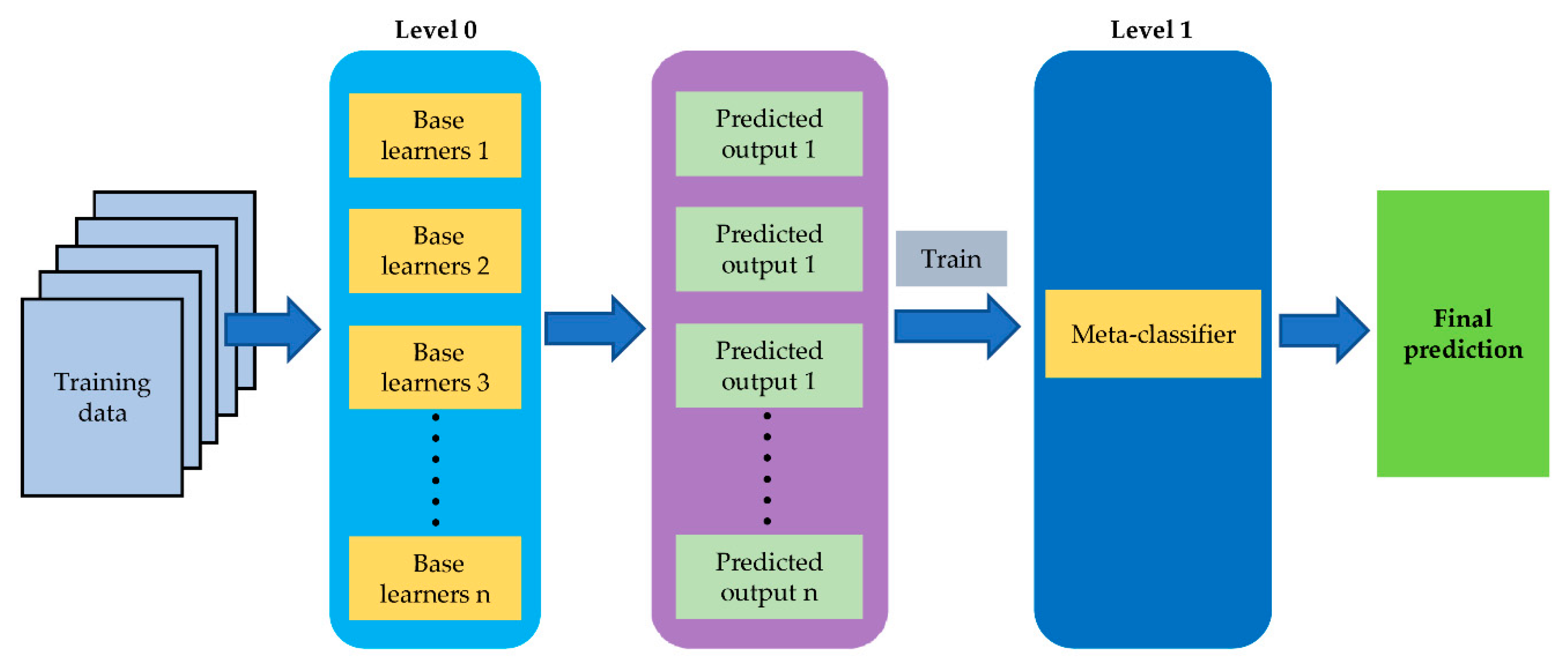
2.4. Model Stacking for Sample Classification

Although most of the models that were based on data sets of Ven-NIR and Ven-MIR had high accuracy, it is possible that stacked generalization could establish a model that had a better performance when compared to the individual classifiers. Through comparisons of tge classification results of Section 2.3.1 and Section 2.3.2, it could be found that RF and SVM appear to be the most effective of individual classifiers, realizing the highest classification rates in many cases when compared to KNN. Confusion matrices that correspond to Ven-NIR-RF, Ven-NIR-SVM, Ven-MIR-RF, and Ven-MIR-SVM shows that the predicted outputs of the two algorithms might be complementary (Supplementary Materials Tables S1–S36). All of the results suggest that the two learners would be the best combination of base learners. Accordingly, RF and SNV models as level-0 base learners were employed in our stacked generalization. Additionally, RF, SNV, and KNN algorithms were used at level-1 learners, respectively. In the final, a total of six scenarios were performed with stacking experiments (

Table 9. The major parameters (accuracy and kappa) of the stacking models.

Scenario	Data Set	Model	Level 1	Calibration Set	Validation Set
				Total ACC (%)	Total ACC (%)	K
A	Ven-NIR	SG-Ven-NIR- RF	RF	100.00	98.61	0.99
B	Ven-NIR	SG-Ven-NIR- SVM	SVM	100.00	97.22	0.97
C	Ven-NIR	SG-Ven-NIR- KNN	KNN	100.00	95.83	0.96
D	Ven-MIR	SG-Ven-MIR- RF	RF	100.00	94.44	0.94
E	Ven-MIR	SG-Ven-MIR- SVM	SVM	100.00	100.00	1.00
F	Ven-MIR	SG-Ven-MIR- KNN	KNN	100.00	90.28	0.90

Note: base learners (level-0) of all stacking models were RF and SNV models

). Additonally, Figure 9 shows the schemes for stacked generalization.

For the Ven-NIR data set (101 variables), the best performing classifier was scenario A. The next best-performing classifiers were scenario B and C, respectively. For the Ven-MIR data set (73 variables), a model of scenario E showed the highest classification rates and second were scenario D and F (94.00% and 90.00% classification rate respectively). Comparing the performance of different stacking models (Table 9 and Supplementary Materials Tables S37–S42), SVM comes out to be the best algorithm at level-1. Additionally, the stacking model, based on the Ven-MIR data set, had the highest accuracy of calibrations and validations sets. The comprehensive analysis revealed that the SVM stacking model combined with the Ven-MIR data set had the best performance (SG-Ven-MIR-SVM).

2.5. Are Model Stacking Better than Data Fusion for Gentiana Species Discrimination?

Presently, the application of stacked generalization for establishing classification models of different medicinal plants or herbs is rather scarce. On the contrary, another modeling approach, data fusion strategy, has been widely used for classification and geographical origin traceability of herbs and foods [48,49,53,54]. Some researches stated that spectra data fusion, such as low-level and mid-level fusion strategies, could improve the discrimination capacity of the classification models and those strategies were usually more efficient than single spectroscopic techniques for modeling [48,49]. We select the Ven-MIR-SG-SVM model in the last section of the research to compare with six data fusion models on prediction accuracy and validate the advantage of stacked generalization in the classification of Gentiana species.

In this study, the FT-MIR and NIR spectral signals were straightforwardly concatenated and they constitute a low-level fusion data set (a total of 2701 variables: the total number of the points in the both MIR and NIR spectra). The mid-level data fusion data set (174 variables) was made up of feature important variables from Ven-NIR (101 variables) and Ven-MIR (73 variables) subsets (Figure 10). Finally, the low- and mid-level data fusion matrices were used to establish the RF, SVM, and KNN models, respectively (

Table 10. The major parameters (accuracy and kappa) of the data fusion models.

Data Fusion Strategy	Number of Variables	Models	Calibration Set	Validation Set
			Total ACC (%)	Total ACC (%)	K
Low-level fusion	2701	Low-RF	100.00	97.22	0.97
Low-level fusion	2701	Low-SVM	100.00	100.00	1.00
Low-level fusion	2701	Low-KNN	100.00	97.22	0.97
Mid-level fusion	174	Mid-RF	100.00	100.00	1.00
Mid-level fusion	174	Mid-SVM	100.00	100.00	1.00
Mid-level fusion	174	Mid-KNN	100.00	100.00	1.00

and Tables S43–S48). For low-level data fusion, the order of successful classification rates of three algorithms was as follows: SVM > RF and KNN. The SVM model resulted in a total accuracy of 100%. Additionlly, the validation set accuracy of RF and KNN were both 97.22%. In the case of mid-level fusion, the SVM model still achieved a total accuracy rate of 100%. In addition, the parameters of RF and KNN models that were based on feature fusion data set of FT-MIR and NIR spectra were higher than that of low-level data fusion.

The low and mid-level data fusion approach improved the discrimination capacity of the developed models to classify Gentiana samples, as shown in Table 10. Among the six classification models that were based on data fusion strategy, Low-SVM, Mid-RF, Mid-SVM, and Mid-KNN were the best performing model according to accuracy, kappa coefficient, and other indicators. When compared with these models, the performance of SG-Ven-MIR-SVM was as good as them (Table 9 and Table 10). The experimental results that were obtained from the two different modeling strategies showed that both model stacking and data fusion could result in a classification model with improved accuracy and enhanced robustness. Additionally, the strategy of stacked generalization could obtain efficient classification models that are as good as data fusion by fewer variables.

As we know, the data fusion (low-level and mid-level) approaches present a fusion of all variables or most important variables (feature variables) to create a model in order to exploit the synergy of the multispectral information to obtain an optimized model [53,54,55,56]. However, the calculation time might be higher when increasing variables. In contrast, stacked generalization reduces the calculation time and keeps fewer variables by combining several different classification algorithms into one meta-model [57,58,59]. In the case of discrimination of Gentiana and its relatives, only 73 variables used in the SG-Ven-MIR-SVM model, while low-level and mid-level data fusion models utilized 2701 and 174 variables for modeling, respectively. The variables number and modeling results indicated that the stacked generalization strategy is probably an important technique for improving species classification model predictive accuracy and avoiding overfitting.

3. Materials and Methods

3.1. Plant Material Collection

The 18 species used in the study belong to two genera (Gentiana and Tripterospermum) of Gentianaceae (Figure 11). All of the species were collected and identified during the flowering and fruiting time of 2018 and 2019. The voucher specimens of those plants were deposited in the College of Chemistry, Biological and Environment, Yuxi Normal University, Yu’xi, China. Their collection location is shown in

Table 11. Source of 180 Gentian and Tripterospermum species samples.

Class	Genus	Species	Geographical Location
1	Gentiana	G. rigescens	Yongde, Lincang, Yunnan, China
2	Gentiana	G. cephalantha	Xuyong, Luzhou, Sichuan, China
3	Gentiana	G. davidii	Jianghua, Yongzhou, Hunan, China
4	Gentiana	G. lawrencei var. farreri	Songpan, Aba, Sichuan, China
5	Gentiana	G. stragulata	Songpan, Aba, Sichuan, China
6	Gentiana	G. crassicaulis	Lanping, Nujiang, Yunnan, China
7	Gentiana	G. loureirii	Jianghua, Yongzhou, Hunan, China
8	Gentiana	G. napulifera	Liping, QianDong-nan, Guizhou, China
9	Gentiana	G. praticola	Liping, QianDong-nan, Guizhou, China
10	Gentiana	G. piasezkii	Ningqiang, Hanzhong, Shaanxi, China
11	Gentiana	G. squarrosa	Songpan, Aba, Sichuan, China
12	Gentiana	G. pseudosquarrosa	Songpan, Aba, Sichuan, China
13	Gentiana	G. rubicunda	Xianfeng, Enshi, Hubei, China
14	Gentiana	G. rubicunda var. samolifolia	Wufeng, Yichang, Hubei, China
15	Gentiana	G. rhodantha	Nayong, Bijie, Guizhou, China
16	Gentiana	G. striata	Songpan, Aba, Sichuan, China
17	Tripterospermum	T. chinense	Tonggu, Yichun, Jiangxi, China
18	Tripterospermum	T. cordatum	Tonggu, Yichun, Jiangxi, China

and medicinal use in southwest China was summarized in

Table 12. Sample information including their application in southwest of China.

Species	Chinese Name	Disease	Ch.P.
G. rigescens	Dian Longdan	heat-clearing, liver protection, icterohepatitis, Japanese encephalitis, cephalalgia, swelling and pain of eye [9,13]	listed (2015 edition) [9]
G. cephalantha	Tou hua Longdan	heat-clearing, icterohepatitis	unlisted
G. davidii	Wu ling Longdan	heat-clearing, urinary tract infection, conjunctivitis [13]	unlisted
G. lawrencei var. farreri	Xian ye Longdan	trachitis, cough, smallpox [13]	unlisted
G. stragulata	Shi e Longdan	none reported	unlisted
G. crassicaulis	Cu jing qin jiao	heat-clearing, icterohepatitis, hematochezia, rheumatism [9]	listed (2015 edition) [9]
G. loureirii	Hua nan Longdan	heat-clearing, icterohepatitis, diarrhea, swelling and pain of eye [13]	unlisted
G. napulifera	Fu gen Longdan	none reported	unlisted
G. praticola	Cao dian Longdan	heat-clearing, detumescence analgesic [13]	unlisted
G. piasezkii	Shan nan Longdan	none reported	unlisted
G. squarrosa	Lin ye Longdan	heat-clearing, acute appendicitis, swelling and pain of eye [13]	unlisted
G. pseudosquarrosa	Jia lin ye Longdan	none reported	unlisted
G. rubicunda	Shen hong Longdan	dyspepsia, bone fracture, snakebite, diminish inflammation [13]	unlisted
G. rubicunda var. samolifolia	Xiao fan lu ye Longdan	none reported	unlisted
G. rhodantha	Hong hua Longdan	heat-clearing, diminish inflammation, urinary tract infection, cold, icterohepatitis, diarrhea, scald [9,13]	listed (2015 edition) [9]
G. striata	Tiao wen Longdan	none reported	unlisted
T. chinense	Shuang hudie	heat-clearing, phthisis, pulmonary abscess, irregular menstruation [13]	unlisted
T. cordatum	E mei Shuang hudie	bone fracture [13]	unlisted

.

In the laboratory, the fresh materials were authenticated. Subsequently, the samples were wash cleaning and dried at 50 °C as soon as possible. The dried whole plant was broken into powder with high-speed disintegrator. Finally, 180 powder samples were collected (10 powder samples per species). All sample powders were screened through a 100-mesh stainless sieve to obtain same-sized particles. The powders after sieving were stored in dry zip-lock bags for a further spectra scan of NIR and FT-MIR.

3.2. Near Infrared (FT-NIR)

The samples were scanned in the Antaris II spectrometer (Thermo Fisher Scientific, Madison, WI, USA). Each powdered sample was scanned from 10,000 to 4000 cm⁻¹ with a resolution of 4 cm⁻¹ until 16 scans were averaged.

3.3. Fourier Transform Mid Infrared (FT-MIR)

The FT-MIR spectrum was recorded using a FT-IR spectrometer (Perkin Elmer, Norwalk, CT, USA) that was equipped with a deuterated triglycine sulfate (DTGS) detector and a ZnSe ATR (attenuated total reflection) accessory (PIKE technologies, Inc. Madison, WI, USA). The spectral fingerprint of every sample was recorded bands from 4000–600 cm⁻¹ while using a resolution of 4 cm⁻¹ and an accumulation of 16 scans. The ATR accessory is equipped with a unique metal O-ring for sample holding in order to control the path length and thickness of the sample (Figure 12). In the beginning, the metal O-ring was placed on the reflection diamond of accessory, and then the sample powder was put on the central of O-ring metal. At last, a pressure tower on the top of the metal O-ring was used to press the powder tightly until a constant pressure (131 ± 1 bar on the scale of the micrometric pressure device) [60]. Before each measurement, a laboratory air spectrum was recorded and checked for remaining water and sample residues, as well as background deduction.

Spectrum signals from 2500 to 1800 cm⁻¹ were not considered for further analysis due to strong crystal absorbance [61]. Furthermore, spectral regions that 4000–3700 cm⁻¹ (baseline area and did not provide relevant information) and 682–653 cm⁻¹ (disturbing absorption band of CO₂) were excluded prior to chemometric analysis [62].

3.4. Statistical Analysis

The principal component analysis (PCA), unsupervised technique, has been widely applied in data dimension reduction and exploratory data analysis [37,63]. From PCA-loading analysis, we can also extract the characteristic variables, which lead to differences between the samples. Additionally, in general, the more important the band corresponding to the spectral variable, the larger PCA-loading value. In this study, PCA was applied to test whether the NIR and FT-MIR spectra fingerprint can result in a clustering of 180 samples and analyze the similarity and dissimilarity in spectra data between species, which might be useful for further understanding phytochemical diversity among different species. Furthermore, the results of PCA would provide reference information for the creation of classification models based while using the supervised technique.

Random forests (RF) or decision tree forests is an ensemble learning technique [64]. This algorithm is based on a combination of a large set of classification and regression trees [64]. After the ensemble of trees (the forest), each tree gives a classification. Finally, the model uses a vote to combine the trees’ predictions [64]. RF can handle extremely large datasets and deal with the “curse of dimensionality” well. Therefore, RF is robust to over-fitting, noise, and outliers, and always performs well in problems with a low feature ratio [65]. All of those indicate that RF is quite competitive relative to other ensemble learning techniques.

The support vector machine (SVM) algorithm is a non-parametric supervised classification [66]. Many previous studies have reported the theory and detailed mathematical explanation of this algorithm [67]. As one of the most robust and accurate data mining algorithms, SVM has been implemented in many programming languages, including R, MATLAB, and so on, which has led SVM to be adopted by a much wider audience. In recent years, SVM has successfully been applied to a number of applications, such as classification of species or geographical origin traceability of food [53,68,69]. It is important to note that SVM can achieve high classification accuracy whlie using a small number of training samples [56,67]. Additionally, it is also a suitable classifier for high-dimensional data [53,69].

The k-nearest neighbors (KNN) algorithm is a distance-based non-parametric discriminant technique [70]. As its name, this algorithm uses information regarding an example’s k-nearest neighbors to classify unlabeled examples and assign one of them to the most common class among the k-nearest neighbors [70]. KNN has been widely used in statistical applications and it has been one of the most successful supervised classification algorithms, especially for the task of multi-class classification [31,71].

Hyperparameters of RF (n_tree and m_try), SVM (kernel function and cost function), and KNN (k) were optimized by using Bayesian optimization of mlr package combined with the MMCE model [50]. The lower MMCE, the hyperparameter was better [50].

Feature selection (“optimal wavenumbers” for classification modeling) is a critical step in the modeling process [72]. There might be some irrelevant or noisy features in data sets because of the infrared techniques provide multivariate and non-specific signals [72,73]. Feature selection of NIR and FT-MIR subsets was based on five methods. The first four were VIP (features were selected by the PLS-DA combined with VIP value) [49], Boruta (features were selected by the Boruta algorithm) [49], GARF (features were selected by the genetic algorithm combined with RF model), and GASVM (features were selected by the genetic algorithm combined with SVM model) [50]. The last was Venn, which feature variables were the intersection of the results of the first four feature selection.

3.5. Model Stacking and Data Fusion

Stacked generalization (stacking) is one of the ensemble learning [43]. The essence of the method is combined predictions from a number of base learners (level 0 models) to generate a more powerful meta-model (level 1 models), with the aim of reducing the generalization error [43,44,45]. Hence, stacked generalization is an ensemble learning method with two or more levels models. The greatest advantage of stacked generalization is the free choice of base learners. Additionally, in general, the classification results of base learners might be complementarities and this combination might be helpful in improving the performance of the final meta-model [44]. Hence, investigating the best methods for constructing the ensemble classifiers was one focus of stacking.

In our study, the first level (level-0) of stacking model is composed of several weak classifiers (base learners 1, base learners 2, base learners 3, base learners n) [45]. Subsequently, the predicted probabilities of basic learners are used to train the second level model (final model) [45]. Figure 9 shows the schemes for stacked generalization.

Unlike stacked generalization, the data fusion strategy focus is on improving the model through best combine the subset. Most of the reported data fusion strategies include low-level data fusion and mid-level data fusion (feature-level data fusion) [48,53].

Low-level data fusion, as its name suggests, subsets are straightforwardly concatenated and reconstitute an independent data matrix. Subsequently, the new dataset is used to establish the classification models [53]. In the case of mid-level data fusion, classification models were established by a new data set, which were formed by concatenating the feature important variables from a subset by different feature selection algorithms [53]. In the research, the low- and mid-level data fusion strategies were considered. Additionally, Figure 10 shows the schemes for data fusion strategies.

3.6. Model Evaluation

The values of TP (Correctly identified samples of positive class), TN (correctly identified samples of negative class), FN (incorrectly identified samples of positive class), and FP (incorrectly identified samples of negative class) were calculated according to the confusion matrices of the classification models [49]. Subsequently, SE, SP, EFF, ACC, MCC, and K were calculated using Equations (1) to (6).

$$\mathrm{ACC}=\frac{\left(\mathrm{TN}+\mathrm{TP}\right)}{\left(\mathrm{TP}+\mathrm{TN}+\mathrm{FP}+\mathrm{FN}\right)}$$

(1)

$$\mathrm{SE}=\frac{\mathrm{TP}}{\left(\mathrm{TP}+\mathrm{FN}\right)}$$

(2)

$$\mathrm{SP}=\frac{\mathrm{TN}}{\left(\mathrm{TN}+\mathrm{FP}\right)}$$

(3)

$$\mathrm{EFF}=\sqrt{\mathrm{SE}\times \mathrm{SP}}$$

(4)

$$\mathrm{MCC}=\frac{\left(\mathrm{TP}\times \mathrm{TN}-\mathrm{FP}\times \mathrm{FN}\right)}{\sqrt{\left(\mathrm{TP}+\mathrm{FP}\right)\left(\mathrm{TP}+\mathrm{FN}\right)\left(\mathrm{TN}+\mathrm{FP}\right)\left(\mathrm{TN}+\mathrm{FN}\right)}}$$

(5)

$$\mathrm{kappa}=\frac{\left(\mathrm{Po}-\mathrm{Pe}\right)}{\left(1-\mathrm{Pe}\right)}$$

(6)

Po: observed agreement value, Pe: expected agreement value.

3.7. Software

ATR correction of the FT-MIR spectra was completed by OMNIC 9.7.7 software (Thermo Fisher Scientific, Madison, WI, USA). The other spectral data preprocessing (SNV and 2nd derivative), PCA, and VIP analysis were performed by SIMCA-P⁺ 14.0 Software (Umetrics AB, Umea, Sweden). In the study, a strategy of two levels stacked generalization was used and the models were developed with R [50]. Kennard–Stone algorithm was used to set the calibration sets and validation sets of all models (MATLAB, Version R 2017a, Mathworks, Natick, MA, USA). The RF, SVM, KNN technique, and feature selection of classification models were all implemented in R software (version 3.6.1, https://www.r-project.org/) base on randomForest, e1071, Boruta, mlr, and class package. The Venn diagrams were completed by the tools on BMKCloud (www.biocloud.net).

4. Conclusions

The results of this study indicated that NIR and FT-MIR spectroscopic techniques combined with chemometrics could successfully discriminate Chinese medicinal Gentiana and their related species. Exploratory data analysis showed the NIR and FT-MIR spectroscopy indirect reflection interspecific phytochemistry diversity of medicinal Gentiana among the genera level and species level. Hence, there was a potential application value of NIR and FT-MIR fingerprint for the identification of medicinal Gentiana and its related species. Subsequently, supervised methods of pattern recognition were used for further analysis of spectra data. Firstly, six classification models based on RF, SVM and KNN algorithms were built on the full spectra data set that was obtained by the NIR and FT-MIR spectroscopy technique, respectively. The FT-MIR-SVM model performed more effectively than other classification models. Five approaches were applied to select optimal wavenumbers in order to improve the performance of the models and filter irrelevant or noisy features in data sets. In the end, the stacking models were built by stacked generalization combined with NIR and FT-MIR feature data sets. The modeling results suggest that RF and SVM were the best combinations of base learners (level-0). When compared the performance of six stacking models, SVM comes out to be the best algorithm at level 1 and the stacking model using the Ven-MIR data set had the highest accuracy of calibrations and validation sets. In conclusion, stacked generalization combined with feature selection is probably an important technique for improving the classification model predictive accuracy and to avoid overfitting.

References

1. Ho, T.N.; James, S.P. Flora of China (Gentianaceae through Boraginaceae); Science Press, Beijing and Missouri Botanical Garden Press: St. Louis, MO, USA, 1995; Volume 16. [Google Scholar]
2. Pan, Y.; Zhao, Y.L.; Zhang, J.; Li, W.Y.; Wang, Y.Z. Phytochemistry and pharmacological activities of the genus Gentiana (Gentianaceae). Chem. Biodivers. 2016, 13, 107–150. [Google Scholar] [CrossRef]
3. Mirzaee, F.; Hosseini, A.; Jouybari, H.B.; Davoodi, A.; Azadbakht, M. Medicinal, biological and phytochemical properties of Gentiana species. J. Tradit. Complement. Med. 2017, 7, 400–408. [Google Scholar] [CrossRef] [PubMed]
4. Mustafa, A.M.; Caprioli, G.; Dikmen, M.; Kaya, E.; Maggi, F.; Sagratini, G.; Vittori, S.; Öztürk, Y. Evaluation of neuritogenic activity of cultivated, wild and commercial roots of Gentiana lutea L. J. Funct. Foods 2015, 19, 164–173. [Google Scholar] [CrossRef]
5. Mustafa, A.M.; Caprioli, G.; Ricciutelli, M.; Maggi, F.; Marín, R.; Vittori, S.; Sagratini, G. Comparative HPLC/ESI-MS and HPLC/DAD study of different populations of cultivated, wild and commercial Gentiana lutea L. Food Chem. 2015, 174, 426–433. [Google Scholar] [CrossRef]
6. Wang, Y.M.; Xu, M.; Wang, D.; Zhu, H.T.; Yang, C.R.; Zhang, Y.J. Review on “Long-Dan”, one of the traditional Chinese medicinal herbs recorded in Chinese pharmacopoeia. Nat. Prod. Bioprospect. 2012, 2, 1–10. [Google Scholar] [CrossRef] [Green Version]
7. Kletter, C.; Glasl, S.; Thalhammer, T.; Narantuya, S. Traditional Mongolian medicine—A potential for drug discovery. Sci. Pharm. 2008, 76, 49–64. [Google Scholar] [CrossRef] [Green Version]
8. Yang, B.; Kim, S.; Kim, J.; Lim, C.; Kim, H.; Cho, S. Gentiana scabra Bunge roots alleviates skin lesions of contact dermatitis in mice. J. Ethnopharmacol. 2019, 233, 141–147. [Google Scholar] [CrossRef]
9. China Pharmacopoeia Committee. Pharmacopoeia of the People’s Republic of China; China Medicinal Science Press: Beijing, China, 2015. [Google Scholar]
10. Xu, Y.; Li, Y.; Maffucci, K.; Huang, L.F.; Zeng, R. Analytical methods of phytochemicals from the Genus Gentiana. Molecules 2017, 22, 2080. [Google Scholar] [CrossRef] [Green Version]
11. Huang, J.; Pei, S.Q.; Long, C.L. An ethnobotanical study of medicinal plants used by the Lisu people in Nujiang, Northwest Yunnan, China. Econ. Bot. 2004, 58, S253–S264. [Google Scholar]
12. Pei, S.J.; Hamilton, A.C.; Yang, L.X.; Hua, H.Y.; Yang, Z.W.; Gao, F.; Zhang, Q.X. Conservation and development through medicinal plants: A case study from Ludian (Northwest Yunnan, China) and presentation of a general model. Biodivers. Conserv. 2010, 19, 2619–2636. [Google Scholar]
13. Yunnan Pharmaceutical Co., Ltd. List of Traditional Chinese Medicine Resources in Yunnan, China; China Science Press: Beijing, China, 1993. [Google Scholar]
14. Zhang, X.X.; Zhan, G.Q.; Jin, M.; Zhang, H.; Dang, J.; Zhang, Y.; Guo, Z.J.; Ito, Y. Botany, traditional use, phytochemistry, pharmacology, quality control, and authentication of Radix Gentianae Macrophyllae-A traditional medicine: A review. Phytomedicine 2018, 46, 142–163. [Google Scholar] [CrossRef] [PubMed]
15. Hou, S.B.; Wang, X.; Huang, R.; Liu, H.M.; Hu, H.; Hu, W.Y.; Lv, S.T.; Zhao, H.; Chen, G. Seven new chemical constituents from the roots of Gentiana macrophylla pall. Fitoterapia 2020, 141, 104476. [Google Scholar] [CrossRef] [PubMed]
16. Gao, L.J.; Li, J.Y.; Qi, J.H. Gentisides A and B, two new neuritogenic compounds from the traditional Chinese medicine Gentiana rigescens Franch. Bioorgan. Med. Chem. 2010, 18, 2131–2134. [Google Scholar] [CrossRef] [PubMed]
17. Gao, L.J.; Xiang, L.; Luo, Y.; Wang, G.F.; Li, J.Y.; Qi, J.H. Gentisides C-K: Nine new neuritogenic compounds from the traditional Chinese medicine Gentiana rigescens Franch. Bioorgan. Med. Chem. 2010, 18, 6995–7000. [Google Scholar] [CrossRef] [PubMed]
18. Liu, M.; Li, X.W.; Liao, B.S.; Luo, L.; Ren, Y.Y. Species identification of poisonous medicinal plant using DNA barcoding. Chin. J. Nat. Medicines 2019, 17, 585–590. [Google Scholar] [CrossRef]
19. Liu, J.; Yang, H.F.; Ge, X.J. The use of DNA barcoding on recently diverged species in the genus Gentiana (Gentianaceae) in China. PLoS ONE 2016, 11, e0153008. [Google Scholar] [CrossRef]
20. Tao, Z.; Jian, W.; Jia, Y.; Li, W.L.; Xu, F.S.; Wang, X.M. Comparative chloroplast genome analyses of species in Gentiana section Cruciata (Gentianaceae) and the development of authentication markers. Int. J. Mol. Sci. 2018, 19, 1962. [Google Scholar]
21. Zheng, P.; Zhang, K.J.; Wang, Z.Z. Genetic diversity and gentiopicroside content of four Gentiana species in China revealed by ISSR and HPLC methods. Biochem. Syst. Ecol. 2011, 39, 704–710. [Google Scholar] [CrossRef]
22. Liu, F.F.; Wang, Y.M.; Zhu, H.T.; Wang, D.; Yang, C.R.; Xu, M.; Zhang, Y.J. Comparative study on “Long-Dan”, “Qin-Jiao” and their adulterants by HPLC Analysis. Nat. Prod. Bioprospect. 2014, 4, 297–308. [Google Scholar] [CrossRef] [Green Version]
23. Pan, Y.; Zhang, J.; Zhao, Y.L.; Wang, Y.Z.; Jin, H. Chemotaxonomic studies of nine Gentianaceae species from western China based on liquid chromatography tandem mass spectrometry and Fourier transform infrared spectroscopy. Phytochem. Analysis 2016, 27, 158–167. [Google Scholar] [CrossRef]
24. Ercioglu, E.; Velioglu, H.M.; Boyaci, I.H. Chemometric evaluation of discrimination of Aromatic plants by Using NIRS, LIBS. Food Anal Method 2018, 11, 1656–1667. [Google Scholar] [CrossRef]
25. Zhang, H.; Chen, Z.Y.; Li, T.H.; Chen, N.; Xu, W.J.; Liu, S.P. Surface-enhanced Raman scattering spectra revealing the inter-cultivar differences for Chinese ornamental Flos Chrysanthemum: A new promising method for plant taxonomy. Plant Methods 2017, 13, 92. [Google Scholar] [CrossRef]
26. Luna, A.S.; Da Silva, A.P.; Da Silva, C.S.; Lima, I.C.A.; de Gois, J.S. Chemometric methods for classification of clonal varieties of green coffee using Raman spectroscopy and direct sample analysis. J. Food Compos. Anal. 2019, 76, 44–50. [Google Scholar] [CrossRef]
27. Lang, C.; Almeida, D.R.A.; Costa, F.R.C. Discrimination of taxonomic identity at species, genus and family levels using Fourier transformed near-infrared Spectroscopy (FT-NIR). Forest. Ecol. Manag. 2017, 406, 219–227. [Google Scholar] [CrossRef]
28. Guzmán, Q.J.A.; Rivard, B.; Sánchez-Azofeifa, G.A. Discrimination of liana and tree leaves from a neotropical dry forest using visible-near infrared and longwave infrared reflectance spectra. Remote Sens. Environ. 2018, 219, 135–144. [Google Scholar] [CrossRef]
29. Borraz-Martínez, S.; Boqué, R.; Simó, J.; Mestre, M.; Gras, A. Development of a methodology to analyze leaves from Prunus dulcis varieties using near infrared spectroscopy. Talanta 2019, 204, 320–328. [Google Scholar] [CrossRef] [PubMed]
30. Meenu, M.; Xu, B.J. Application of vibrational spectroscopy for classification, authentication and quality analysis of mushroom: A concise review. Food Chem. 2019, 289, 545–557. [Google Scholar] [CrossRef]
31. Chen, Y.F.; Chen, Y.; Feng, X.P.; Yang, X.F.; Zhang, J.N.; Qiu, Z.J.; He, Y. Variety identification of Orchids using Fourier transform infrared spectroscopy combined with stacked sparse auto-encoder. Molecules 2019, 13, 2506. [Google Scholar] [CrossRef] [Green Version]
32. Liu, R.H.; Sun, Q.F.; Hu, T.; Li, L.; Nie, L.; Wang, J.Y.; Zhou, W.H.; Zang, H.C. Multi-parameters monitoring during traditional Chinese medicine concentration process with near infrared spectroscopy and chemometrics. Spectrochim. Acta A 2018, 192, 75–81. [Google Scholar] [CrossRef]
33. Liu, P.; Wang, J.; Li, Q.; Gao, J.; Tan, X.Y.; Bian, X.Y. Rapid identification and quantification of Panax notoginseng with its adulterants by near infrared spectroscopy combined with chemometrics. Spectrochim. Acta A 2019, 206, 23–30. [Google Scholar] [CrossRef]
34. Sousa, C.; Quintelas, C.; Augusto, C.; Ferreira, E.C.; Páscoa, R.N.M.J. Discrimination of Camellia japonica cultivars and chemometric models: An interlaboratory study. Comput. Electron. Agr. 2019, 159, 28–33. [Google Scholar] [CrossRef] [Green Version]
35. Wang, Y.; Zuo, Z.T.; Huang, H.Y.; Wang, Y.Z. Original plant traceability of Dendrobium species using multi-spectroscopy fusion and mathematical models. Roy. Soc. Open. Sci. 2019, 6, 190399. [Google Scholar] [CrossRef] [PubMed] [Green Version]
36. Wu, X.M.; Zuo, Z.T.; Zhang, Q.Z.; Wang, Y.Z. Classification of Paris species according to botanical and geographical origins based on spectroscopic, chromatographic, conventional chemometric analysis and data fusion strategy. Microchem. J. 2018, 143, 367–378. [Google Scholar] [CrossRef]
37. Li, T.; Su, C. Authenticity identification and classification of Rhodiola species in traditional Tibetan medicine based on Fourier transform near-infrared spectroscopy and chemometrics analysis. Spectrochim. Acta A 2018, 204, 131–140. [Google Scholar] [CrossRef] [PubMed]
38. Wang, Y.Y.; Li, J.Q.; Liu, H.G.; Wang, Y.Z. Attenuated total reflection-Fourier transform infrared spectroscopy (ATR-FTIR) combined with chemometrics methods for the classification of Lingzhi species. Molecules 2019, 24, 2210. [Google Scholar] [CrossRef] [PubMed] [Green Version]
39. Pasquini, C. Near infrared spectroscopy: A mature analytical technique with new perspectives—A review. Anal. Chim. Acta 2018, 1026, 8–36. [Google Scholar] [CrossRef]
40. Yun, Y.H.; Li, H.D.; Deng, B.C.; Cao, D.S. An overview of variable selection methods in multivariate analysis of near-infrared spectra. TrAC Trend. Anal. Chem. 2019, 113, 102–115. [Google Scholar] [CrossRef]
41. Yang, X.D.; Li, G.L.; Song, J.; Gao, M.J.; Zhou, S.L. Rapid discrimination of Notoginseng powder adulteration of different grades using FT-MIR spectroscopy combined with chemometrics. Spectrochim. Acta A 2018, 205, 457–464. [Google Scholar] [CrossRef]
42. Li, Y.; Zhang, J.Y.; Wang, Y.Z. FT-MIR and NIR spectral data fusion: A synergetic strategy for the geographical traceability of Panax notoginseng. Anal. Bioanal. Chem. 2018, 410, 91–103. [Google Scholar] [CrossRef]
43. Wolpert, D.H. Stacked generalization. Neural Networks 1992, 5, 241–259. [Google Scholar] [CrossRef]
44. Naimi, A.I.; Balzer, L.B. Stacked generalization: An introduction to super learning. Eur. J. Epidemiol. 2018, 33, 459–464. [Google Scholar] [CrossRef] [PubMed]
45. Alexandropoulos, S.A.N.; Aridas, C.K.; Kotsiantis, S.B.; Vrahatis, M.N. Stacking strong ensembles of classifiers. In Nonlinear Model Predictive Control; Springer Science and Business Media LLC: Berlin, Germany, 2019; pp. 545–556. [Google Scholar]
46. Shan, P.; Zhao, Y.; Wang, Q.; Sha, X.; Lv, X.; Peng, S.; Ying, Y. Stacked ensemble extreme learning machine coupled with Partial Least Squares-based weighting strategy for nonlinear multivariate calibration. Spectrochim. Acta A 2019, 215, 97–111. [Google Scholar] [CrossRef] [PubMed]
47. Sfakianakis, S.; Bei, E.S.; Zervakis, M. Stacking of network based vlassifiers with application in breast cancer classification. In XIV Mediterranean Conference on Medical and Biological Engineering and Computing; Kyriacou, E., Christofides, S., Pattichis, C., Eds.; Springer: Berlin, Germany, 2016. [Google Scholar]
48. Wang, Q.Q.; Huang, H.Y.; Wang, Y.Z. Geographical authentication of Macrohyporia cocos by a data fusion method combining ultra-fast liquid chromatography and Fourier transform infrared spectroscopy. Molecules 2019, 24, 1320. [Google Scholar] [CrossRef] [PubMed] [Green Version]
49. Pei, Y.; Zuo, Z.T.; Zhang, Q.Z.; Wang, Y.Z. Data fusion of fourier transform mid-infrared (MIR) and near-infrared (NIR) spectroscopies to identify geographical origin of wild Paris polyphylla var. yunnanensis. Molecules 2019, 24, 2559. [Google Scholar] [CrossRef] [Green Version]
50. Bischl, B.; Lang, M.; Kotthoff, L.; Schiffne, J.; Richter, J.; Studerus, E.; Casalicchio, G.; Jones, Z.M. mlr: Machine Learning in R. J. Mach. Learn. Res. 2016, 17, 5938–5942. [Google Scholar]
51. Chen, W.; Pourghasemi, H.R.; Naghibi, S.A. A comparative study of landslide susceptibility maps produced using support vector machine with different kernel functions and entropy data mining models in China. B. Eng. Geol. Environ. 2018, 77, 647–664. [Google Scholar] [CrossRef]
52. Qian, Y.G.; Zhou, W.Q.; Yan, J.L.; Li, W.F.; Han, L.J. Comparing machine learning classifiers for object-based land cover classification using very high resolution imagery. Remote Sens. 2015, 7, 153–168. [Google Scholar] [CrossRef]
53. Li, Y.; Zhang, J.; Li, T.; Liu, H.G.; Li, J.Q.; Wang, Y.Z. Geographical traceability of wild Boletus edulis based on data fusion of FT-MIR and ICP-AES coupled with data mining methods (SVM). Spectrochim. Acta A 2017, 177, 20–27. [Google Scholar] [CrossRef]
54. Li, L.Q.; Xie, S.M.; Ning, J.M.; Chen, Q.S.; Zhang, Z.Z. Evaluating green tea quality based on multisensor data fusion combining hyperspectral imaging and olfactory visualization systems. J. Sci. Food Agr. 2019, 99, 1787–1794. [Google Scholar] [CrossRef]
55. Schwolow, S.; Gerhardt, N.; Rohn, S.; Weller, P. Data fusion of GC-IMS data and FT-MIR spectra for the authentication of olive oils and honeys—is it worth to go the extra mile? Anal. Bioanal. Chem. 2019, 411, 6005–6019. [Google Scholar] [CrossRef]
56. Ríos-Reina, R.; Callejón, R.M.; Savorani, F.; Amigo, J.M.; Cocchi, M. data fusion approaches in spectroscopic characterization and classification of PDO wine vinegars. Talanta 2019, 198, 560–572. [Google Scholar] [CrossRef] [Green Version]
57. Tsakiridis, N.L.; Tziolas, N.V.; Theocharis, J.B.; Zalidis, G.C. A genetic algorithm-based stacking algorithm for predicting soil organic matter from vis–NIR spectral data. Eur. J. Soil. Sci. 2019, 70, 578–590. [Google Scholar] [CrossRef]
58. Verma, A.K.; Pal, S. Prediction of skin disease with three different feature selection techniques using stacking ensemble method. Appl. Biochem. Biotech. 2019, 1, 1–20. [Google Scholar] [CrossRef]
59. Zhang, Y.; Zhang, R.R.; Ma, Q.F.; Wang, Y.H.; Wang, Q.Q.; Huang, Z.H.; Huang, L.Y. A feature selection and multi-model fusion-based approach of predicting air quality. ISA T. 2019. [Google Scholar] [CrossRef]
60. Wang, Y.; Huang, H.Y.; Zuo, Z.T.; Wang, Y.Z. Comprehensive quality assessment of Dendrubium officinale using ATR-FTIR spectroscopy combined with random forest and support vector machine regression. Spectrochim. Acta A 2018, 205, 637–648. [Google Scholar] [CrossRef]
61. Rodríguez, S.D.; Rolandelli, G.; Buera, M.P. Detection of quinoa flour adulteration by means of FT-MIR spectroscopy combined with chemometric methods. Food Chem. 2019, 274, 392–401. [Google Scholar] [CrossRef]
62. Horn, B.; Esslinger, S.; Pfister, M.; Fauhl-Hassek, C.; Riedl, J. Non-targeted detection of paprika adulteration using mid-infrared spectroscopy and one-class classification–Is it data preprocessing that makes the performance? Food Chem. 2018, 257, 112–119. [Google Scholar] [CrossRef]
63. Mees, C.; Souard, F.; Delporte, C.; Deconinck, E.; Stoffelen, P.; Stévigny, C.; Kauffmann, J.; De Braekeleer, K. Identification of coffee leaves using FT-NIR spectroscopy and SIMCA. Talanta 2018, 177, 4–11. [Google Scholar] [CrossRef]
64. Breiman, L. Random Forests. Mach. Learn. 2001, 45, 5–32. [Google Scholar] [CrossRef] [Green Version]
65. De Santana, F.B.; Mazivila, S.J.; Gontijo, L.C.; Neto, W.B.; Poppi, R.J. Rapid Discrimination between authentic and adulterated andiroba oilusing FTIR-HATR spectroscopy and Random Forest. Food Anal. Method 2018, 11, 1927–1935. [Google Scholar] [CrossRef]
66. Chapelle, O.; Patrick, H.; Vladimir, N.V. Support vector machines for histogram-based image classification. IEEE Trans. Neural Netw. 1999, 10, 1055–1064. [Google Scholar] [CrossRef]
67. Belousov, A.I.; Verzakov, S.A.; von Frese, J. A flexible classification approach with optimal generalisation performance: Support vector machines. Chemometr. Intell. Lab. 2002, 64, 15–25. [Google Scholar] [CrossRef]
68. Ballanti, L.; Blesius, L.; Hines, E.; Kruse, B. Tree species classification using hyperspectral imagery: A comparison of two classifiers. Remote Sens-Basel. 2016, 6, 445. [Google Scholar] [CrossRef] [Green Version]
69. Yang, Y.; Wu, Y.J.; Li, W.L.; Liu, X.S.; Zheng, J.Y.; Zhang, W.T.; Chen, Y. Determination of geographical origin and icariin content of Herba Epimedii using near infrared spectroscopy and chemometrics. Spectrochim. Acta A 2018, 191, 233–240. [Google Scholar] [CrossRef]
70. Altman, N.S. An Introduction to Kernel and Nearest-Neighbor Nonparametric Regression. Am. Stat. 1992, 46, 175–185. [Google Scholar]
71. Sharma, P.; Aggarwal, A.; Gupta, A.; Garg, A. Leaf identification using HOG, KNN, and neural networks. In International Conference on Innovative Computing and Communications; Bhattacharyya, S., Hassanien, A., Gupta, D., Khanna, A., Pan, I., Eds.; Springer: Berlin, Germany, 2019. [Google Scholar]
72. Mehmood, T.; Liland, K.H.; Snipen, L.; Sæbø, S. A review of variable selection methods in partial least squares regression. Chemometr. Intell. Lab. 2012, 118, 62–69. [Google Scholar] [CrossRef]
73. Casale, M.; Casolino, C.; Oliveri, P.; Forina, M. The potential of coupling information using three analytical techniques for identifying the geographical origin of Liguria extra virgin olive oil. Food Chem. 2010, 118, 163–170. [Google Scholar] [CrossRef]
Sample Availability: Samples of the compound are not available from the authors.
Figure 1. Raw near-infrared (NIR) (A) and Fourier transform mid-infrared (FT-MIR) (B) spectra of 180 samples of G. rigescens and its related species.
Molecules 25 01442 g001
Figure 2. Averaged NIR spectra of 18 species of Gentiana (A), (B) and Tripterospermum species (C).
Molecules 25 01442 g002
Figure 3. Averaged FT-MIR spectra of 18 Gentiana (A), (B), and Tripterospermum species (C).
Molecules 25 01442 g003
Figure 4. Score plots of PCA for 180 samples using NIR spectra after pretreatment (A) score plot of PC1 vs. PC2, (B) score plot of PC1 vs. PC3. The meaning of the codes (1–18) could be found in the sample information.
Molecules 25 01442 g004
Figure 5. Score plots of PCA for 180 samples using FT-MIR spectra after pretreatment (A) score plot of PC1 vs. PC2, (B) score plot of PC1 vs. PC3. The meaning of the codes (1–18) could be found in the sample information.
Molecules 25 01442 g005
Figure 6. Feature selection strategies in the study.
Molecules 25 01442 g006
Figure 7. Size of feature variables of the four algorithms (A) feature selection of NIR spectroscopy, (B) feature selection of FT-MIR spectroscopy.
Molecules 25 01442 g007
Figure 8. Venn diagram representing the overlap of the selected feature variables by variable importance in projection (VIP), Boruta, genetic algorithm combined with random forest (GARF), and genetic algorithm combined with support vector machine (GASVM) algorithms (A) Venn diagram calculate based on feature selection results of NIR variables, (B) Venn diagram calculate based on feature selection results of FT-MIR variables.
Molecules 25 01442 g008
Figure 9. Stacked generalization in the study.
Molecules 25 01442 g009
Figure 10. The low-level and mid-level data fusion strategies in the study.
Molecules 25 01442 g010
Figure 11. Medicinal Gentiana and its relatives in the study.
Molecules 25 01442 g011
Figure 12. ZnSe ATR accessory (left) and the metal O-ring (right) in the study.
Molecules 25 01442 g012