
Molecular Modeling and Design Studies of Purine Derivatives as Novel CDK2 Inhibitors

Abstract
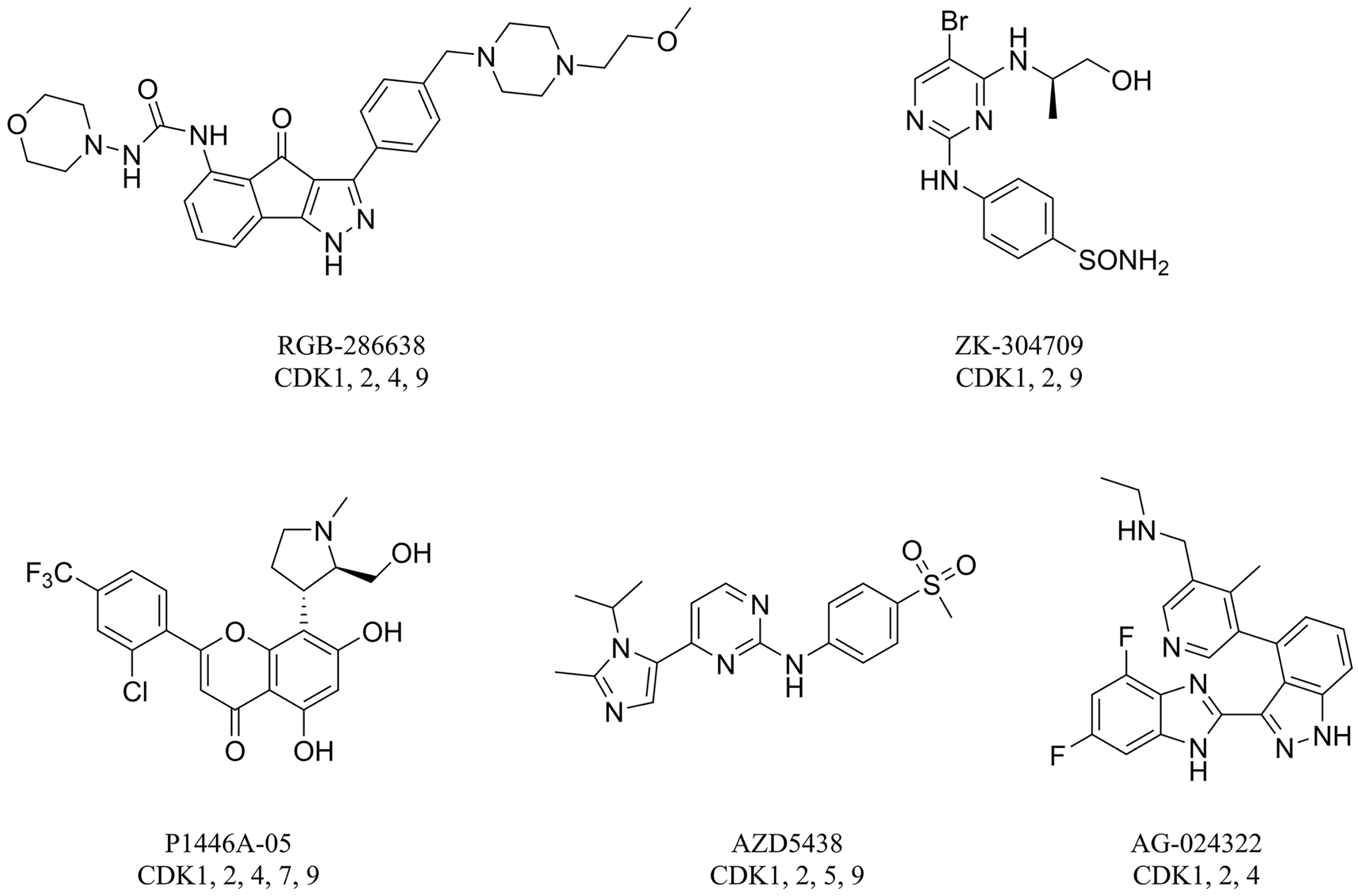
1. Introduction
2. Results and Discussion
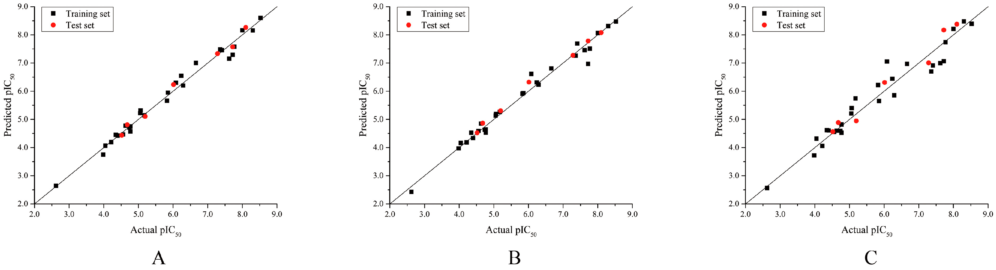
2.1. Validation of 3D-QSAR Models
2.2. 3D-QSAR Statistical Analysis
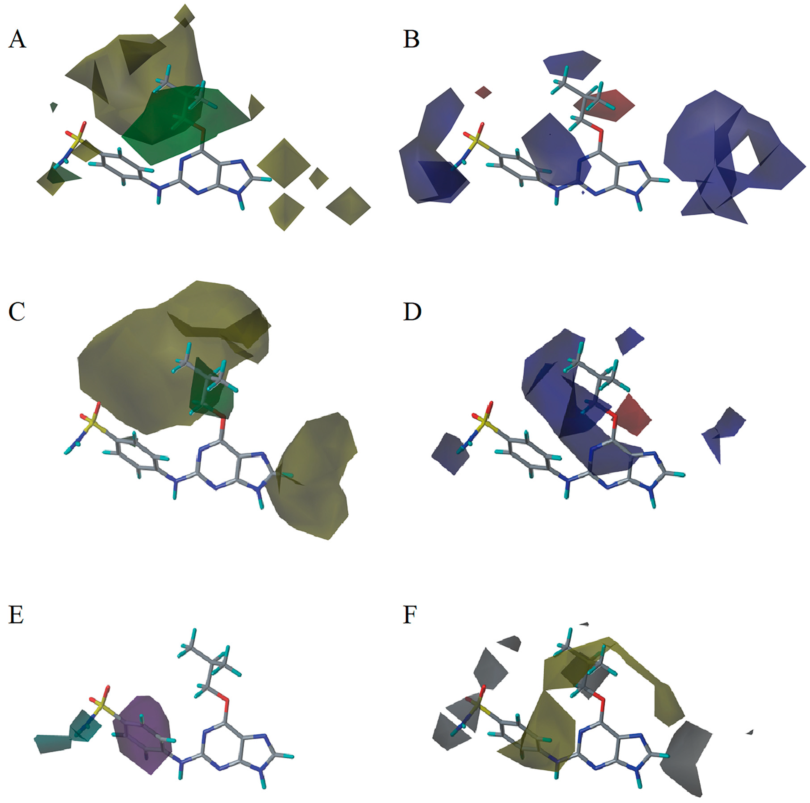
2.3. 3D-QSAR Model Contour Map Analysis
2.4. Virtual Screening Results and Molecular Design
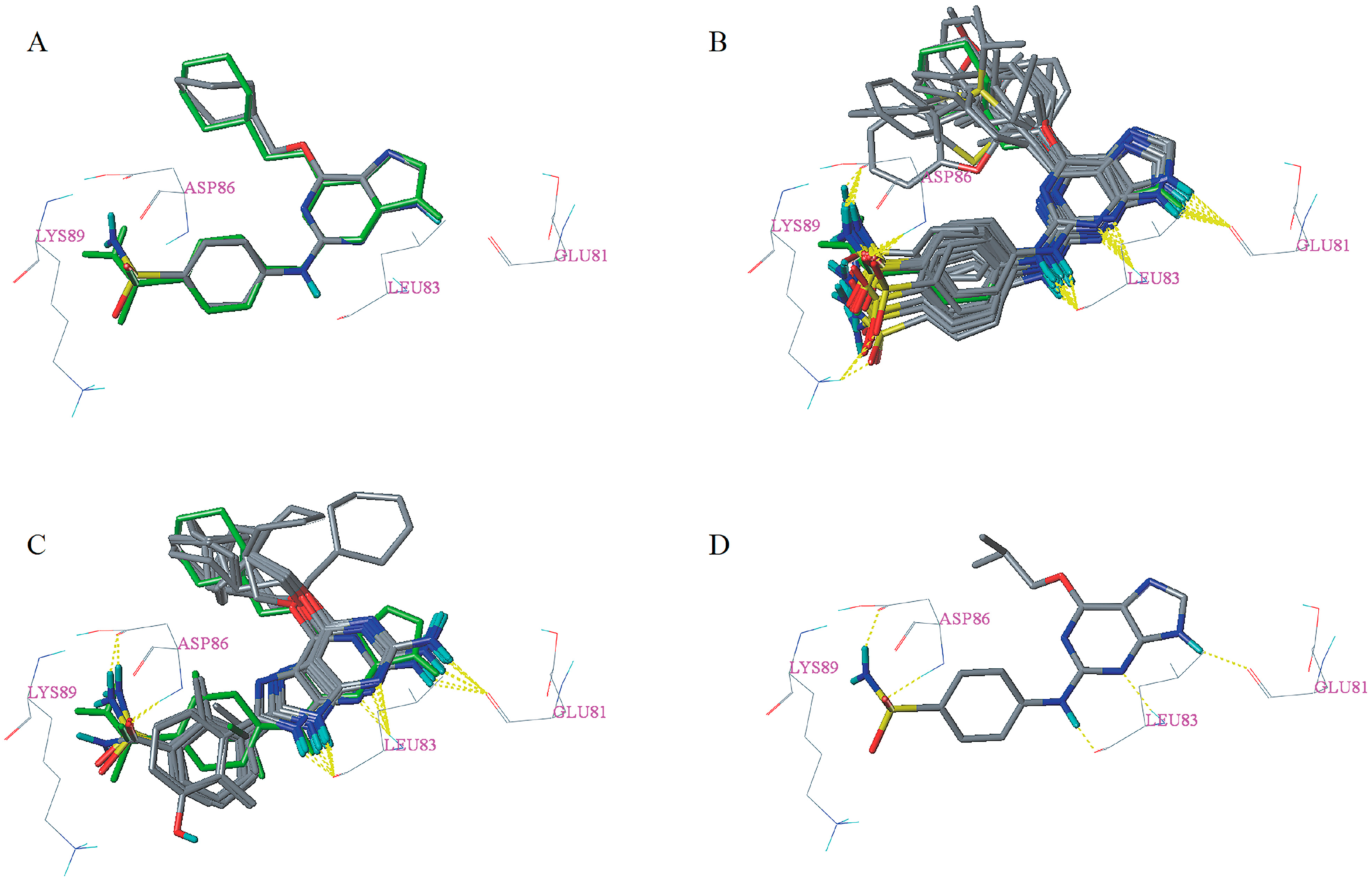
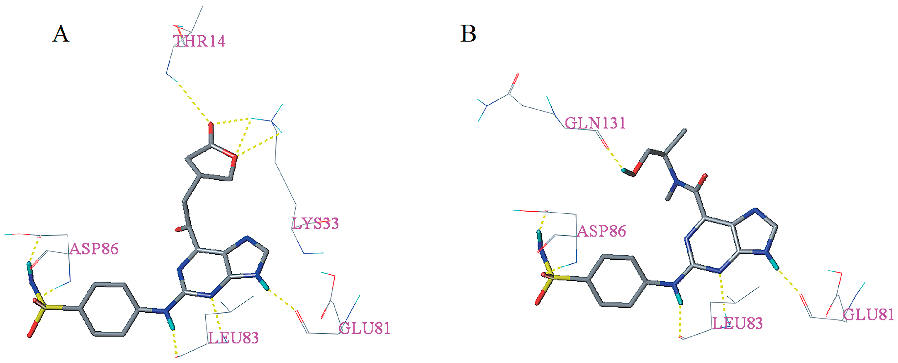
2.5. Docking Analysis
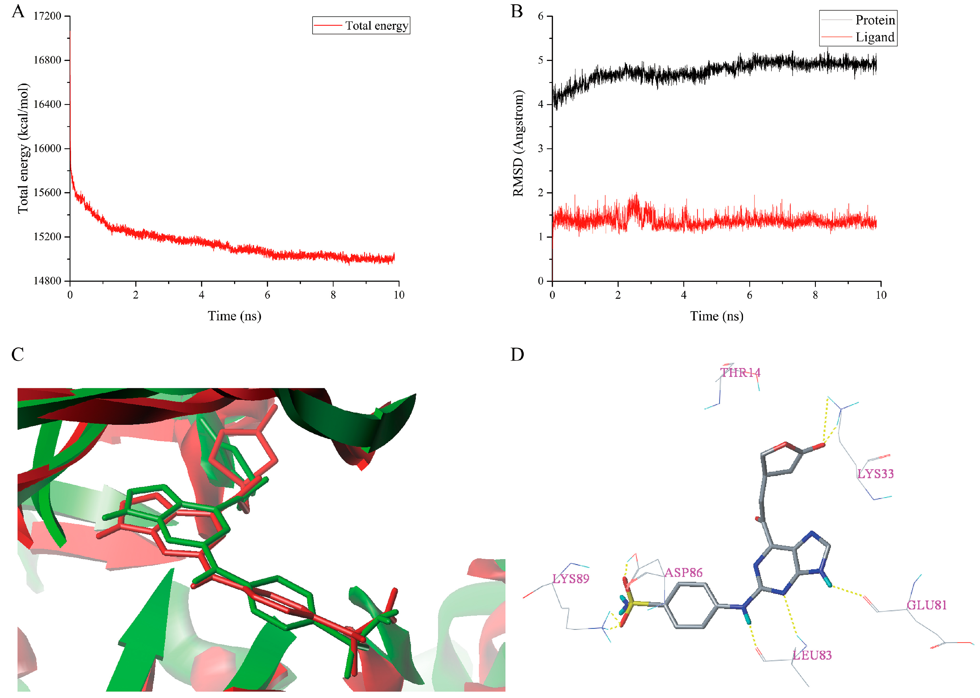
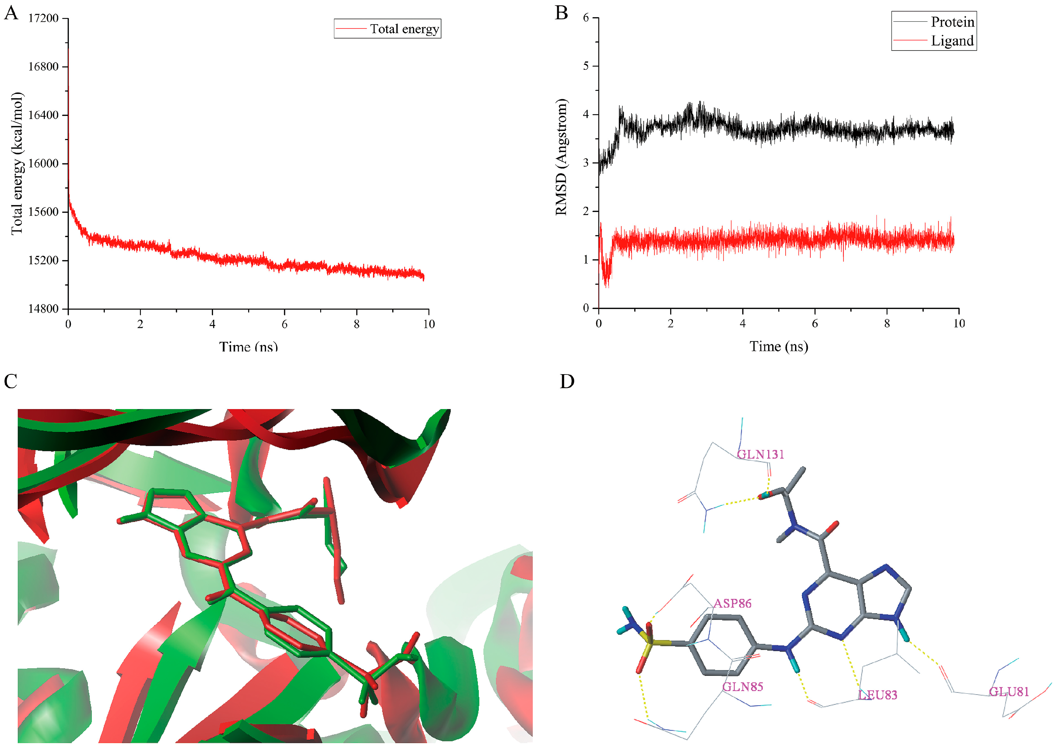
2.6. MD Simulations Analysis
3. Materials and Methods
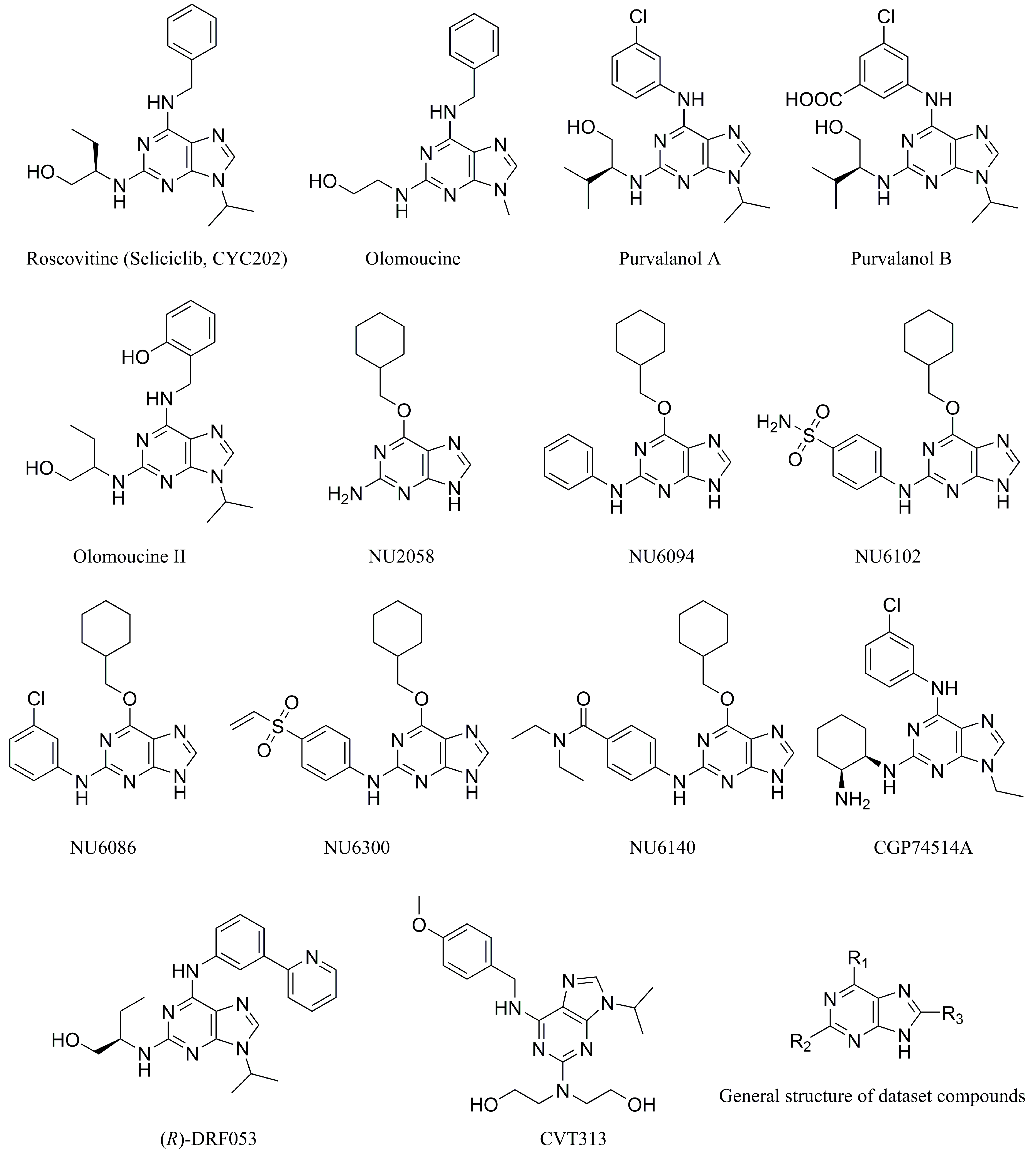
3.1. Dataset
3.2. Structure Preparation
3.3. Molecular Docking
3.4. Alignment
3.5. Creation of CoMFA and CoMSIA Models
3.6. Partial Least Squares Analysis
3.7. Creation of Topomer CoMFA Model
3.8. Validation of 3D-QSAR Models
3.9. Virtual Screening
3.10. MD Simulations
4. Conclusions
Supplementary Materials
Author Contributions
Funding
Conflicts of Interest
References
- Hanahan, D.; Weinberg, R.A. Hallmarks of cancer: The next generation. Cell 2011, 144, 646–674. [Google Scholar] [CrossRef] [PubMed]
- Whittaker, S.R.; Mallinger, A.; Workman, P.; Clarke, P.A. Inhibitors of cyclin-dependent kinases as cancer therapeutics. Pharmacol. Ther. 2017, 173, 83–105. [Google Scholar] [CrossRef] [PubMed]
- Sánchez-Martínez, C.; Gelbert, L.M.; Lallena, M.J.; de Dios, A. Cyclin dependent kinase (CDK) inhibitors as anticancer drugs. Bioorg. Med. Chem. Lett. 2015, 25, 3420–3435. [Google Scholar] [CrossRef] [PubMed]
- Weinberg, R.A. The retinoblastoma protein and cell cycle control. Cell 1995, 81, 323–330. [Google Scholar] [CrossRef]
- Malumbres, M. Cyclin-dependent kinases. Genome Biol. 2014, 15, 122. [Google Scholar] [CrossRef] [PubMed]
- Malumbres, M.; Barbacid, M. Cell cycle, CDKs and cancer: A changing paradigm. Nat. Rev. Cancer 2009, 9, 153–166. [Google Scholar] [CrossRef] [PubMed]
- Chohan, T.; Qian, H.; Pan, Y.; Chen, J.-Z. Cyclin-dependent kinase-2 as a target for cancer therapy: Progress in the development of CDK2 inhibitors as anti-cancer agents. Curr. Med. Chem. 2015, 22, 237–263. [Google Scholar] [CrossRef] [PubMed]
- Asghar, U.; Witkiewicz, A.K.; Turner, N.C.; Knudsen, E.S. The history and future of targeting cyclin-dependent kinases in cancer therapy. Nat. Rev. Drug Discov. 2015, 14, 130–146. [Google Scholar] [CrossRef] [PubMed]
- Davies, T.G.; Bentley, J.; Arris, C.E.; Boyle, F.T.; Curtin, N.J.; Endicott, J.A.; Gibson, A.E.; Golding, B.T.; Griffin, R.J.; Hardcastle, I.R.; et al. Structure-based design of a potent purine-based cyclin-dependent kinase inhibitor. Nat. Struct. Biol. 2002, 9, 745–749. [Google Scholar] [CrossRef] [PubMed]
- Jorda, R.; Hendrychova, D.; Voller, J.; Reznickova, E.; Gucky, T.; Krystof, V. How selective are pharmacological inhibitors of cell-cycle-regulating cyclin-dependent kinases? J. Med. Chem. 2018, 61, 9105–9120. [Google Scholar] [CrossRef] [PubMed]
- Anscombe, E.; Meschini, E.; Mora-Vidal, R.; Martin, M.P.; Staunton, D.; Geitmann, M.; Danielson, U.H.; Stanley, W.A.; Wang, L.Z.; Reuillon, T.; et al. Identification and characterization of an irreversible inhibitor of CDK2. Chem. Biol. 2015, 22, 1159–1164. [Google Scholar] [CrossRef] [PubMed]
- Carbain, B.; Paterson, D.J.; Anscombe, E.; Campbell, A.J.; Cano, C.; Echalier, A.; Endicott, J.A.; Golding, B.T.; Haggerty, K.; Hardcastle, I.R.; et al. 8-Substituted O(6)-cyclohexylmethylguanine CDK2 inhibitors: Using structure-based inhibitor design to optimize an alternative binding mode. J. Med. Chem. 2014, 57, 56–70. [Google Scholar] [CrossRef] [PubMed]
- Coxon, C.R.; Anscombe, E.; Harnor, S.J.; Martin, M.P.; Carbain, B.; Golding, B.T.; Hardcastle, I.R.; Harlow, L.K.; Korolchuk, S.; Matheson, C.J.; et al. Cyclin-dependent kinase (CDK) inhibitors: Structure-activity relationships and insights into the CDK-2 selectivity of 6-substituted 2-arylaminopurines. J. Med. Chem. 2017, 60, 1746–1767. [Google Scholar] [CrossRef] [PubMed]
- Cramer, R.D.; Patterson, D.E.; Bunce, J.D. Comparative molecular field analysis (CoMFA). 1. Effect of shape on binding of steroids to carrier proteins. J. Am. Chem. Soc. 1988, 110, 5959–5967. [Google Scholar] [CrossRef] [PubMed]
- Klebe, G.; Abraham, U.; Mietzner, T. Molecular similarity indices in a comparative analysis (CoMSIA) of drug molecules to correlate and predict their biological activity. J. Med. Chem. 1994, 37, 4130–4146. [Google Scholar] [CrossRef] [PubMed]
- Cramer, R.D. Topomer CoMFA: A design methodology for rapid lead optimization. J. Med. Chem. 2003, 46, 374–388. [Google Scholar] [CrossRef] [PubMed]
- Cramer, R.D.; Jilek, R.J.; Guessregen, S.; Clark, S.J.; Wendt, B.; Clark, R.D. “Lead hopping”. Validation of topomer similarity as a superior predictor of similar biological activities. J. Med. Chem. 2004, 47, 6777–6791. [Google Scholar] [CrossRef] [PubMed]
- Tropsha, A.; Gramatica, P.; Gombar, V.K. The importance of being earnest: Validation is the absolute essential for successful application and interpretation of QSPR models. QSAR Comb. Sci. 2003, 22, 69–77. [Google Scholar] [CrossRef]
- Zitzler, E.; Thiele, L. Multiobjective evolutionary algorithms: A comparative case study and the strength Pareto approach. IEEE Trans. Evolut. Comput. 1999, 3, 257–271. [Google Scholar] [CrossRef]
- Clark, R.D.; Fox, P.C. Statistical variation in progressive scrambling. J. Comput. Aided Mol. Des. 2004, 18, 563–576. [Google Scholar] [CrossRef] [PubMed]
- Yuan, H.; Liu, H.; Tai, W.; Wang, F.; Zhang, Y.; Yao, S.; Ran, T.; Lu, S.; Ke, Z.; Xiong, X.; et al. Molecular modelling on small molecular CDK2 inhibitors: An integrated approach using a combination of molecular docking, 3D-QSAR and pharmacophore modelling. SAR QSAR Environ. Res. 2013, 24, 795–817. [Google Scholar] [CrossRef] [PubMed]
- Roy, K.; Das, R.N.; Ambure, P.; Aher, R.B. Be aware of error measures. Further studies on validation of predictive QSAR models. Chemom. Intell. Lab. Syst. 2016, 152, 18–33. [Google Scholar] [CrossRef]
- Tong, J.-B.; Bai, M.; Zhao, X. Application of an R-group search technique into molecular design of HIV-1 integrase inhibitors. J. Serb. Chem. Soc. 2016, 81, 383–394. [Google Scholar] [CrossRef]
- Kramer, B.; Rarey, M.; Lengauer, T. Evaluation of the FLEXX incremental construction algorithm for protein-ligand docking. Proteins 1999, 37, 228–241. [Google Scholar] [CrossRef]
- Pham, T.A.; Jain, A.N. Parameter estimation for scoring protein-ligand interactions using negative training data. J. Med. Chem. 2006, 49, 5856–5868. [Google Scholar] [CrossRef] [PubMed]
- Chaube, U.; Chhatbar, D.; Bhatt, H. 3D-QSAR, molecular dynamics simulations and molecular docking studies of benzoxazepine moiety as mTOR inhibitor for the treatment of lung cancer. Bioorg. Med. Chem. Lett. 2016, 26, 864–874. [Google Scholar] [CrossRef] [PubMed]
- Patel, S.; Patel, B.; Bhatt, H. 3D-QSAR studies on 5-hydroxy-6-oxo-1,6-dihydropyrimidine-4-carboxamide derivatives as HIV-1 integrase inhibitors. J. Taiwan Inst. Chem. Eng. 2016, 59, 61–68. [Google Scholar] [CrossRef]
- Jain, A.N. Morphological similarity: A 3D molecular similarity method correlated with protein-ligand recognition. J. Comput. Aided Mol. Des. 2000, 14, 199–213. [Google Scholar] [CrossRef] [PubMed]
- Lorca, M.; Morales-Verdejo, C.; Vasquez-Velasquez, D.; Andrades-Lagos, J.; Campanini-Salinas, J.; Soto-Delgado, J.; Recabarren-Gajardo, G.; Mella, J. Structure-activity relationships based on 3D-QSAR CoMFA/CoMSIA and design of aryloxypropanol-amine agonists with selectivity for the human beta3-adrenergic receptor and anti-obesity and anti-diabetic profiles. Molecules 2018, 23, 1191. [Google Scholar] [CrossRef] [PubMed]
- Clark, M.; Cramer, R.D.; Van Opdenbosch, N. Validation of the general purpose tripos 5.2 force field. J. Comput. Chem. 1989, 10, 982–1012. [Google Scholar] [CrossRef]
- Powell, M.J.D. Restart procedures for the conjugate gradient method. Math. Program. 1977, 12, 241–254. [Google Scholar] [CrossRef]
- Gasteiger, J.; Marsili, M. Iterative partial equalization of orbital electronegativity—A rapid access to atomic charges. Tetrahedron 1980, 36, 3219–3228. [Google Scholar] [CrossRef]
- Jain, A.N. Surflex: Fully automatic flexible molecular docking using a molecular similarity-based search engine. J. Med. Chem. 2003, 46, 499–511. [Google Scholar] [CrossRef] [PubMed]
- Chaube, U.; Bhatt, H. 3D-QSAR, molecular dynamics simulations, and molecular docking studies on pyridoaminotropanes and tetrahydroquinazoline as mTOR inhibitors. Mol. Divers. 2017, 21, 741–759. [Google Scholar] [CrossRef] [PubMed]
- Cho, S.J.; Tropsha, A. Cross-validated R2-guided region selection for comparative molecular field analysis: A simple method to achieve consistent results. J. Med. Chem. 1995, 38, 1060–1066. [Google Scholar] [CrossRef] [PubMed]
- Zheng, J.; Xiao, G.; Guo, J.; Zheng, Y.; Gao, H.; Zhao, S.; Zhang, K.; Sun, P. Exploring QSARs for 5-lipoxygenase (5-LO) inhibitory activity of 2-substituted 5-hydroxyindole-3-carboxylates by CoMFA and CoMSIA. Chem. Biol. Drug Des. 2011, 78, 314–321. [Google Scholar] [CrossRef] [PubMed]
- Urniaz, R.D.; Jozwiak, K. X-ray crystallographic structures as a source of ligand alignment in 3D-QSAR. J. Chem. Inf. Model. 2013, 53, 1406–1414. [Google Scholar] [CrossRef] [PubMed]
- Romero-Parra, J.; Chung, H.; Tapia, R.A.; Faundez, M.; Morales-Verdejo, C.; Lorca, M.; Lagos, C.F.; Di Marzo, V.; David Pessoa-Mahana, C.; Mella, J. Combined CoMFA and CoMSIA 3D-QSAR study of benzimidazole and benzothiophene derivatives with selective affinity for the CB2 cannabinoid receptor. Eur. J. Pharm. Sci. 2017, 101, 1–10. [Google Scholar] [CrossRef] [PubMed]
- Klebe, G.; Abraham, U. Comparative molecular similarity index analysis (CoMSIA) to study hydrogen-bonding properties and to score combinatorial libraries. J. Comput. Aided Mol. Des. 1999, 13, 1–10. [Google Scholar] [CrossRef] [PubMed]
- Ferrer-Pertuz, K.; Espinoza, L.; Mella, J. Insights into the structural requirements of potent brassinosteroids as vegetable growth promoters using second-internode elongation as biological activity: CoMFA and CoMSIA studies. Int. J. Mol. Sci. 2017, 18, 2734. [Google Scholar] [CrossRef] [PubMed]
- Cramer, R.D.; Bunce, J.D.; Patterson, D.E.; Frank, I.E. Crossvalidation, bootstrapping, and partial least squares compared with multiple regression in conventional QSAR studies. Quant. Struct.-Act. Relat. 1988, 7, 18–25. [Google Scholar] [CrossRef]
- Mella-Raipan, J.; Hernandez-Pino, S.; Morales-Verdejo, C.; Pessoa-Mahana, D. 3D-QSAR/CoMFA-based structure-affinity/selectivity relationships of aminoalkylindoles in the cannabinoid CB1 and CB2 receptors. Molecules 2014, 19, 2842–2861. [Google Scholar] [CrossRef] [PubMed]
- Tong, J.; Wu, Y.; Bai, M.; Zhan, P. 3D-QSAR and molecular docking studies on HIV protease inhibitors. J. Mol. Struct. 2017, 1129, 17–22. [Google Scholar] [CrossRef]
- Bush, B.L.; Nachbar, R.B., Jr. Sample-distance partial least squares: PLS optimized for many variables, with application to CoMFA. J. Comput. Aided Mol. Des. 1993, 7, 587–619. [Google Scholar] [CrossRef] [PubMed]
- Tong, J.-B.; Bai, M.; Zhao, X. 3D-QSAR and docking studies of HIV-1 protease inhibitors using R-group search and Surflex-dock. Med. Chem. Res. 2016, 25, 2619–2630. [Google Scholar] [CrossRef]
- Tong, J.-B.; Li, Y.-Y.; Jiang, G.-Y.; Li, K.-N. Application of an R-group search technique in the molecular design of dipeptidyl boronic acid proteasome inhibitors. J. Serb. Chem. Soc. 2017, 82, 1025–1037. [Google Scholar] [CrossRef]
- Ojha, P.K.; Mitra, I.; Das, R.N.; Roy, K. Further exploring rm2 metrics for validation of QSPR models. Chemom. Intell. Lab. Syst. 2011, 107, 194–205. [Google Scholar] [CrossRef]
- Golbraikh, A.; Tropsha, A. Beware of q2! J. Mol. Graph. Model. 2002, 20, 269–276. [Google Scholar] [CrossRef]
- Pratim Roy, P.; Paul, S.; Mitra, I.; Roy, K. On two novel parameters for validation of predictive QSAR models. Molecules 2009, 14, 1660–1701. [Google Scholar] [CrossRef] [PubMed]
- Irwin, J.J.; Sterling, T.; Mysinger, M.M.; Bolstad, E.S.; Coleman, R.G. ZINC: A free tool to discover chemistry for biology. J. Chem. Inf. Model. 2012, 52, 1757–1768. [Google Scholar] [CrossRef] [PubMed]
- Halgren, T.A. Maximally diagonal force constants in dependent angle-bending coordinates. II. Implications for the design of empirical force fields. J. Am. Chem. Soc. 1990, 112, 4710–4723. [Google Scholar] [CrossRef]
- Berendsen, H.J.C.; Postma, J.P.M.; van Gunsteren, W.F.; DiNola, A.; Haak, J.R. Molecular dynamics with coupling to an external bath. J. Chem. Phys. 1984, 81, 3684–3690. [Google Scholar] [CrossRef]
Sample Availability: Samples of the compounds are not available from the authors. |


| Alignment | Model | ||||
|---|---|---|---|---|---|
| 1 | CoMFA-SE | 0.866 | 0.865 | 0.902 | 0.901 |
| 1 | CoMSIA-HSE | 0.857 | 0.855 | 0.897 | 0.891 |
| 1 | CoMSIA-AHSE | 0.841 | 0.840 | 0.906 | 0.905 |
| 2 | CoMFA-SE | 0.876 | 0.875 | 0.867 | 0.866 |
| 2 | CoMSIA-DHSE | 0.850 | 0.849 | 0.949 | 0.945 |
| 2 | CoMSIA-AHSE | 0.833 | 0.831 | 0.927 | 0.925 |
| 3 | CoMSIA-ASE | 0.816 | 0.817 | 0.829 | 0.856 |
| 3 | CoMSIA-DHS | 0.764 | 0.766 | 0.615 | 0.648 |
| 3 | CoMSIA-DHSE | 0.839 | 0.840 | 0.743 | 0.754 |
| 3 | CoMSIA-AHSE | 0.815 | 0.816 | 0.791 | 0.823 |
| 3 | CoMSIA-DAHSE | 0.831 | 0.832 | 0.806 | 0.831 |
| Parameter | CoMFA | CoMSIA | Topomer CoMFA |
|---|---|---|---|
| 0.991 | 0.990 | 0.962 | |
| 0.991 | 0.994 | 0.971 | |
| 0.999 | 0.996 | 0.992 | |
| 0.999 | 0.997 | 0.992 | |
| ( − )/ | −0.008 | −0.002 | −0.022 |
| ( − )/ | −0.008 | −0.003 | −0.022 |
| k | 0.994 | 0.987 | 0.980 |
| k’ | 1.006 | 1.013 | 1.019 |
| MAE(test) | 0.127 | 0.101 | 0.258 |
| MAE(train) | 0.151 | 0.154 | 0.295 |
| σ(test) | 0.054 | 0.105 | 0.113 |
| σ(train) | 0.121 | 0.155 | 0.229 |
| (test) | 0.902 | 0.949 | 0.831 |
| (test) | 0.901 | 0.945 | 0.830 |
| (avg) | 0.902 | 0.947 | 0.831 |
| ∆(test) | 0.001 | 0.004 | 0.001 |
| Compound | pIC50 | CoMFA | CoMSIA | Topomer CoMFA | |||
|---|---|---|---|---|---|---|---|
| Pred. | Res. | Pred. | Res. | Pred. | Res. | ||
| 1 | 4.770 | 4.570 | 0.200 | 4.530 | 0.240 | 4.815 | −0.045 |
| 2 * | 6.013 | 6.239 | −0.226 | 6.323 | −0.310 | 6.311 | −0.298 |
| 3 | 8.301 | 8.158 | 0.143 | 8.314 | −0.013 | 8.476 | −0.175 |
| 4 | 2.620 | 2.646 | −0.026 | 2.429 | 0.191 | 2.562 | 0.058 |
| 5 | 4.215 | 4.191 | 0.024 | 4.181 | 0.034 | 4.057 | 0.158 |
| 6 | 5.824 | 5.662 | 0.162 | 5.910 | −0.086 | 6.222 | −0.398 |
| 7 * | 8.097 | 8.260 | −0.163 | 8.081 | 0.016 | 8.378 | −0.281 |
| 8 | 8.000 | 8.161 | −0.161 | 8.067 | −0.067 | 8.212 | −0.212 |
| 9 | 8.523 | 8.600 | −0.077 | 8.472 | 0.051 | 8.389 | 0.134 |
| 10 * | 7.721 | 7.575 | 0.146 | 7.782 | −0.061 | 8.172 | −0.451 |
| 11 | 7.770 | 7.582 | 0.188 | 7.511 | 0.259 | 7.740 | 0.030 |
| 12 * | 4.678 | 4.807 | −0.129 | 4.869 | −0.191 | 4.889 | −0.211 |
| 13 | 6.081 | 6.302 | −0.221 | 6.614 | −0.533 | 7.054 | −0.973 |
| 14 * | 5.194 | 5.107 | 0.087 | 5.303 | −0.109 | 4.946 | 0.248 |
| 15 | 5.051 | 5.222 | −0.171 | 5.137 | −0.086 | 5.209 | −0.158 |
| 16 | 6.658 | 7.002 | −0.344 | 6.808 | −0.150 | 6.972 | −0.314 |
| 17 | 7.721 | 7.288 | 0.433 | 6.971 | 0.750 | 7.064 | 0.657 |
| 18 | 7.620 | 7.152 | 0.468 | 7.458 | 0.162 | 6.995 | 0.625 |
| 19 | 7.409 | 7.460 | −0.051 | 7.690 | −0.281 | 6.909 | 0.500 |
| 20 * | 7.284 | 7.335 | −0.051 | 7.271 | 0.013 | 7.006 | 0.278 |
| 21 | 7.357 | 7.481 | −0.124 | 7.260 | 0.097 | 6.700 | 0.657 |
| 22 | 6.237 | 6.547 | −0.310 | 6.313 | −0.076 | 6.442 | −0.205 |
| 23 | 5.854 | 5.948 | −0.094 | 5.936 | −0.082 | 5.651 | 0.203 |
| 24 | 5.174 | 5.142 | 0.032 | 5.264 | −0.090 | 5.746 | −0.572 |
| 25 | 4.350 | 4.449 | −0.099 | 4.528 | −0.178 | 4.619 | −0.269 |
| 26 * | 4.519 | 4.435 | 0.084 | 4.527 | −0.008 | 4.561 | −0.042 |
| 27 | 4.558 | 4.466 | 0.092 | 4.592 | −0.034 | 4.554 | 0.004 |
| 28 | 4.046 | 4.064 | −0.018 | 4.163 | −0.117 | 4.314 | −0.268 |
| 29 | 4.770 | 4.750 | 0.020 | 4.643 | 0.127 | 4.529 | 0.241 |
| 30 | 4.740 | 4.707 | 0.033 | 4.634 | 0.106 | 4.597 | 0.143 |
| 31 | 3.983 | 3.751 | 0.232 | 3.971 | 0.012 | 3.723 | 0.260 |
| 32 | 4.629 | 4.775 | −0.146 | 4.849 | −0.220 | 4.599 | 0.030 |
| 33 | 4.400 | 4.424 | −0.024 | 4.336 | 0.064 | 4.606 | −0.206 |
| 34 | 5.061 | 5.317 | −0.256 | 5.197 | −0.136 | 5.401 | −0.340 |
| 35 | 6.292 | 6.200 | 0.092 | 6.234 | 0.058 | 5.857 | 0.435 |

| Compound | R1 | R2 | R3 | IC50 (µM) or % Inhibition | pIC50 |
|---|---|---|---|---|---|
| 1 |  | –NH2 | –H | 17.000 | 4.770 |
| 2 * |  |  | –H | 0.970 | 6.013 |
| 3 |  |  | –H | 0.005 | 8.301 |
| 4 | –H | –NH2 | –H | 4% a | 2.620 |
| 5 | –H |  | –H | 61.000 | 4.215 |
| 6 | –H |  | –H | 1.500 | 5.824 |
| 7 * |  |  | –H | 0.008 | 8.097 |
| 8 |  |  | –H | 0.010 | 8.000 |
| 9 |  |  | –H | 0.003 | 8.523 |
| 10 * |  |  | –H | 0.019 | 7.721 |
| 11 | –C≡CSi(i-Pr)3 |  | –H | 0.017 | 7.770 |
| 12 * | –C≡CH |  | –H | 21.000 | 4.678 |
| 13 | –C≡CH |  | –H | 0.830 | 6.081 |
| 14 * | –C≡CMe |  | –H | 6.400 | 5.194 |
| 15 | –C≡CPh |  | –H | 8.900 | 5.051 |
| 16 | –Et |  | –H | 0.220 | 6.658 |
| 17 |  |  | –H | 0.019 | 7.721 |
| 18 |  |  | –H | 0.024 | 7.620 |
| 19 |  |  | –H | 0.039 | 7.409 |
| 20 * |  |  | –H | 0.052 | 7.284 |
| 21 |  |  | –H | 0.044 | 7.357 |
| 22 |  |  | –H | 0.580 | 6.237 |
| 23 |  |  | –H | 1.400 | 5.854 |
| 24 |  |  | –H | 6.700 | 5.174 |
| 25 |  | –NH2 | –Me | 44.700 | 4.350 |
| 26 * |  | –NH2 | –Et | 30.300 | 4.519 |
| 27 |  | –NH2 | –i-Pr | 27.700 | 4.558 |
| 28 |  | –NH2 |  | 10% b | 4.046 |
| 29 |  | –NH2 |  | 17.000 | 4.770 |
| 30 |  | –NH2 |  | 18.200 | 4.740 |
| 31 |  | –NH2 | –CF3 | 49% a | 3.983 |
| 32 |  | –NH2 |  | 23.500 | 4.629 |
| 33 |  | –NH2 |  | 39.800 | 4.400 |
| 34 |  | –NH2 |  | 8.700 | 5.061 |
| 35 |  | –NH2 |  | 0.510 | 6.292 |
© 2018 by the authors. Licensee MDPI, Basel, Switzerland. This article is an open access article distributed under the terms and conditions of the Creative Commons Attribution (CC BY) license (http://creativecommons.org/licenses/by/4.0/).
Share and Cite
Zhang, G.; Ren, Y. Molecular Modeling and Design Studies of Purine Derivatives as Novel CDK2 Inhibitors. Molecules 2018, 23, 2924. https://doi.org/10.3390/molecules23112924
Zhang G, Ren Y. Molecular Modeling and Design Studies of Purine Derivatives as Novel CDK2 Inhibitors. Molecules. 2018; 23(11):2924. https://doi.org/10.3390/molecules23112924
Chicago/Turabian StyleZhang, Gaomin, and Yujie Ren. 2018. "Molecular Modeling and Design Studies of Purine Derivatives as Novel CDK2 Inhibitors" Molecules 23, no. 11: 2924. https://doi.org/10.3390/molecules23112924
APA StyleZhang, G., & Ren, Y. (2018). Molecular Modeling and Design Studies of Purine Derivatives as Novel CDK2 Inhibitors. Molecules, 23(11), 2924. https://doi.org/10.3390/molecules23112924