Largely Reduced Grid Densities in a Vibrational Self-Consistent Field Treatment Do Not Significantly Impact the ResultingWavenumbers


Abstract
:
1. Introduction
2. Methods
2.1. Energy Minimization
2.2. Second Derivatives of the Energy
2.3. The VSCF Routine
2.4. Extensions of the VSCF Approach
3. Results and Discussion
3.1. Performance of the PT2-VSCF Approach

| H2O (C2v) | Sym. | 6 | 7 | 8 | 9 | 10 | 11 | 12 | 13 | 14 | 15 | 16 | Expt. [59,71,72] |
|---|---|---|---|---|---|---|---|---|---|---|---|---|---|
| νOH2 ,as | B2 | 2875 | 3997 | 3731 | 3772 | 3766 | 3766 | 3765 | 3765 | 3765 | 3765 | 3765 | 3756 |
| νOH2 ,s | A1 | 3041 | 3785 | 3657 | 3691 | 3684 | 3683 | 3683 | 3682 | 3682 | 3682 | 3682 | 3652 |
| δOH2 | A1 | 1216 | 1688 | 1570 | 1590 | 1586 | 1586 | 1586 | 1586 | 1586 | 1586 | 1586 | 1595 |
| μ | 21.3 | 5.3 | 0.8 | 0.6 | 0.6 | 0.6 | 0.5 | 0.5 | 0.5 | 0.5 | 0.5 | n.a. | |
| CO2 (D∞h) | Sym. | 6 | 7 | 8 | 9 | 10 | 11 | 12 | 13 | 14 | 15 | 16 | Expt. [59,73,74] |
| νCO2,as | 1791 | 2547 | 2359 | 2391 | 2386 | 2386 | 2385 | 2385 | 2385 | 2385 | 2385 | 2349 | |
| νCO2,s | 993 | 1408 | 1255 | 1319 | 1316 | 1315 | 1315 | 1315 | 1315 | 1315 | 1315 | 1285 | |
| δCO2 | ∏μ | 487 | 699 | 645 | 654 | 653 | 653 | 653 | 653 | 653 | 653 | 653 | 667 |
| δCO2 | ∏μ | 487 | 699 | 645 | 654 | 653 | 653 | 653 | 653 | 653 | 653 | 653 | 667 |
| μ | 25.1 | 6.9 | 2.3 | 2.0 | 2.0 | 2.0 | 2.0 | 2.0 | 2.0 | 2.0 | 2.0 | n.a. | |
| CH2O (C2v) | Sym. | 6 | 7 | 8 | 9 | 10 | 11 | 12 | 13 | 14 | 15 | 16 | Expt. [59,75,76,77] |
| νCH2,as | B1 | 2184 | 3000 | 2809 | 2837 | 2833 | 2833 | 2833 | 2832 | 2832 | 2832 | 2832 | 2843 |
| νCH2,s | A1 | 2250 | 2905 | 2801 | 2823 | 2818 | 2818 | 2818 | 2817 | 2817 | 2817 | 2817 | 2782 |
| νCO | A1 | 1312 | 1855 | 1719 | 1745 | 1741 | 1740 | 1740 | 1740 | 1740 | 1740 | 1740 | 1746 |
| δCH2 | A1 | 1157 | 1614 | 1502 | 1521 | 1518 | 1518 | 1518 | 1518 | 1518 | 1518 | 1518 | 1500 |
| ρCH2 | B1 | 945 | 1340 | 1240 | 1257 | 1254 | 1254 | 1254 | 1254 | 1254 | 1254 | 1254 | 1249 |
| ωCH2 | B2 | 891 | 1250 | 1162 | 1176 | 1174 | 1173 | 1173 | 1173 | 1173 | 1173 | 1173 | 1167 |
| μ | 23.0 | 6.4 | 0.8 | 0.8 | 0.7 | 0.7 | 0.7 | 0.7 | 0.7 | 0.7 | 0.7 | n.a. | |
| C2H2 (D∞h) | Sym. | 6 | 7 | 8 | 9 | 10 | 11 | 12 | 13 | 14 | 15 | 16 | Expt. [59,60,78,79,80] |
| νC2H2,s | 2699 | 3490 | 3375 | 3390 | 3384 | 3380 | 3384 | 3384 | 3384 | 3384 | 3384 | 3374 | |
| νC2H2,as | 2523 | 3405 | 3199 | 3233 | 3228 | 3227 | 3227 | 3227 | 3227 | 3227 | 3227 | 3289 | |
| νCC | 1469 | 2046 | 1912 | 1937 | 1932 | 1932 | 1932 | 1932 | 1932 | 1932 | 1932 | 1974 | |
| δC2H2,s | ∏u | 557 | 792 | 733 | 746 | 743 | 743 | 743 | 743 | 743 | 743 | 743 | 730 |
| δC2H2,s | ∏u | 557 | 792 | 733 | 746 | 743 | 743 | 743 | 743 | 743 | 743 | 743 | 730 |
| δC2H2,as | ∏g | 443 | 638 | 589 | 602 | 598 | 598 | 598 | 598 | 598 | 598 | 598 | 612 |
| δC2H2,as | ∏g | 443 | 638 | 589 | 602 | 598 | 598 | 598 | 598 | 598 | 598 | 598 | 612 |
| μ | 24.5 | 5.2 | 2.0 | 1.7 | 1.8 | 1.8 | 1.8 | 1.8 | 1.8 | 1.8 | 1.8 | n.a. | |
| HCOOH (Cs) | Sym. | 6 | 7 | 8 | 9 | 10 | 11 | 12 | 13 | 14 | 15 | 16 | Expt. [59,81,82,83,84] |
| νOH | A' | 2841 | 3682 | 3530 | 3559 | 3550 | 3557 | 3552 | 3552 | 3552 | 3552 | 3552 | 3570 |
| νCH | A' | 2246 | 3134 | 2959 | 2983 | 2978 | 2977 | 2977 | 2977 | 2977 | 2977 | 2977 | 2943 |
| νC=O | A' | 1337 | 1910 | 1764 | 1790 | 1786 | 1786 | 1786 | 1785 | 1785 | 1785 | 1785 | 1770 |
| δCH | A' | 1043 | 1480 | 1367 | 1384 | 1381 | 1381 | 1381 | 1381 | 1381 | 1381 | 1381 | 1387 |
| δOH | A' | 982 | 1367 | 1265 | 1280 | 1277 | 1277 | 1277 | 1277 | 1277 | 1277 | 1277 | 1387 |
| νC-O | A' | 848 | 1148 | 1077 | 1089 | 1086 | 1086 | 1086 | 1086 | 1086 | 1086 | 1086 | 1105 |
| δCH | A" | 786 | 1114 | 1029 | 1042 | 1040 | 1040 | 1040 | 1040 | 1040 | 1040 | 1040 | 1033 |
| δOH,oop | A" | 515 | 631 | 588 | 623 | 609 | 608 | 609 | 609 | 609 | 609 | 609 | 638 |
| δOCO | A' | 469 | 659 | 611 | 619 | 617 | 617 | 617 | 617 | 617 | 617 | 617 | 625 |
| μ | 22.8 | 6.0 | 2.1 | 1.4 | 1.7 | 1.7 | 1.7 | 1.7 | 1.7 | 1.7 | 1.7 | n.a. | |
| CH4 (Td) | Sym. | 6 | 7 | 8 | 9 | 10 | 11 | 12 | 13 | 14 | 15 | 16 | Expt. [59,60,85,86] |
| νCH3,as | F2 | 2333 | 3210 | 3000 | 3035 | 3029 | 3029 | 3028 | 3028 | 3028 | 3028 | 3028 | 3019 |
| νCH3,as | F2 | 2299 | 3177 | 2990 | 3020 | 3015 | 3015 | 3014 | 3014 | 3014 | 3014 | 3014 | 3019 |
| νCH3,as | F2 | 2330 | 3209 | 2999 | 3033 | 3028 | 3027 | 3027 | 3027 | 3027 | 3027 | 3027 | 3019 |
| νCH4,s | A1 | 2588 | 2968 | 2948 | 2943 | 2945 | 2944 | 2943 | 2943 | 2943 | 2943 | 2943 | 2917 |
| δCH4,as | E | 1166 | 1641 | 1523 | 1542 | 1539 | 1539 | 1539 | 1539 | 1539 | 1539 | 1539 | 1534 |
| δCH4,as | E | 1166 | 1641 | 1523 | 1542 | 1539 | 1539 | 1539 | 1539 | 1539 | 1539 | 1539 | 1534 |
| δCH3,s | F2 | 993 | 1390 | 1293 | 1309 | 1306 | 1306 | 1306 | 1306 | 1306 | 1306 | 1306 | 1306 |
| δCH3,s | F2 | 992 | 1390 | 1293 | 1309 | 1306 | 1306 | 1306 | 1306 | 1306 | 1306 | 1306 | 1306 |
| δCH3,s | F2 | 993 | 1390 | 1294 | 1309 | 1307 | 1307 | 1307 | 1306 | 1306 | 1306 | 1306 | 1306 |
| µ | 22.3 | 5.9 | 0.9 | 0.4 | 0.3 | 0.3 | 0.3 | 0.3 | 0.3 | 0.3 | 0.3 | n.a. | |
| CH3Cl (C3v) | Sym. | 6 | 7 | 8 | 9 | 10 | 11 | 12 | 13 | 14 | 15 | 16 | Expt. [59,87,88,89,90] |
| νCH3,as | E | 2338 | 3203 | 3002 | 3035 | 3030 | 3029 | 3029 | 3029 | 3029 | 3029 | 3029 | 3039 |
| νCH3,as | E | 2306 | 3192 | 2974 | 3019 | 3016 | 3015 | 3015 | 3015 | 3015 | 3015 | 3014 | 3039 |
| νCH3,s | A1 | 2339 | 3074 | 2964 | 2989 | 2987 | 2986 | 2986 | 2985 | 2985 | 2985 | 2985 | 2937 |
| δCH3,as | E | 1106 | 1555 | 1445 | 1463 | 1460 | 1460 | 1460 | 1460 | 1460 | 1460 | 1460 | 1452 |
| δCH3,as | E | 1106 | 1556 | 1444 | 1462 | 1460 | 1459 | 1459 | 1459 | 1459 | 1459 | 1459 | 1452 |
| δCH3,s | A1 | 1036 | 1464 | 1357 | 1375 | 1372 | 1372 | 1371 | 1371 | 1371 | 1371 | 1371 | 1355 |
| ρCH3 | E | 773 | 1099 | 1017 | 1031 | 1028 | 1028 | 1028 | 1028 | 1028 | 1028 | 1028 | 1017 |
| ρCH3 | E | 776 | 1099 | 1020 | 1033 | 1031 | 1031 | 1031 | 1031 | 1031 | 1031 | 1031 | 1017 |
| νCCl | A1 | 585 | 802 | 749 | 760 | 758 | 758 | 758 | 758 | 758 | 758 | 758 | 732 |
| µ | 23.0 | 7.0 | 0.9 | 1.4 | 1.2 | 1.2 | 1.2 | 1.2 | 1.2 | 1.2 | 1.2 | n.a. | |
| CH3OH (Cs) | Sym. | 6 | 7 | 8 | 9 | 10 | 11 | 12 | 13 | 14 | 15 | 16 | Expt. [59,60,91,92,93] |
| νOH | A’ | 2812 | 3900 | 3646 | 3694 | 3687 | 3686 | 3686 | 3686 | 3686 | 3686 | 3686 | 3681 |
| νCH3,as | A’ | 2301 | 3198 | 2984 | 3035 | 3030 | 3029 | 3028 | 3028 | 3028 | 3028 | 3028 | 3000 |
| νCH3,as | A” | 2230 | 3091 | 2881 | 2912 | 2908 | 2908 | 2907 | 2907 | 2907 | 2907 | 2907 | 2960 |
| νCH3,s | A’ | 2363 | 2951 | 2849 | 2957 | 2947 | 2942 | 2941 | 2941 | 2941 | 2941 | 2941 | 2844 |
| δCH3,as | A’ | 1130 | 1587 | 1475 | 1493 | 1490 | 1490 | 1490 | 1490 | 1490 | 1490 | 1490 | 1477 |
| δCH3,as | A” | 1116 | 1574 | 1459 | 1478 | 1475 | 1475 | 1475 | 1475 | 1474 | 1474 | 1474 | 1477 |
| δCH3,s | A’ | 1104 | 1563 | 1447 | 1466 | 1463 | 1463 | 1463 | 1463 | 1463 | 1463 | 1463 | 1455 |
| δOH | A’ | 1020 | 1458 | 1342 | 1362 | 1359 | 1359 | 1358 | 1358 | 1358 | 1358 | 1358 | 1345 |
| ρCH3 | A” | 843 | 1178 | 1069 | 1083 | 1081 | 1081 | 1080 | 1080 | 1080 | 1080 | 1080 | 1060 |
| νCO | A’ | 789 | 1060 | 1015 | 1028 | 1026 | 1026 | 1025 | 1025 | 1025 | 1025 | 1025 | 1033 |
| µ | 22.9 | 6.4 | 0.9 | 1.3 | 1.2 | 1.2 | 1.2 | 1.2 | 1.1 | 1.1 | 1.1 | n.a. | |
| CH3CN (C3v) | Sym. | 6 | 7 | 8 | 9 | 10 | 11 | 12 | 13 | 14 | 15 | 16 | Expt. [59,94,95,96,97,98,99,100] |
| νCH3,as | E | 2281 | 3153 | 2940 | 2972 | 2967 | 2967 | 2967 | 2966 | 2966 | 2966 | 2966 | 3009 |
| νCH3,as | E | 2322 | 3172 | 2976 | 2994 | 2990 | 2989 | 2989 | 2988 | 2988 | 2988 | 2988 | 3009 |
| νCH3,s | A1 | 2322 | 3059 | 2951 | 2970 | 2968 | 2967 | 2967 | 2967 | 2967 | 2967 | 2967 | 2954 |
| νCN | A1 | 1656 | 2308 | 2152 | 2178 | 2174 | 2174 | 2173 | 2173 | 2173 | 2173 | 2173 | 2267 |
| δCH3,as | E | 1099 | 1547 | 1438 | 1456 | 1453 | 1453 | 1453 | 1453 | 1453 | 1453 | 1453 | 1454 |
| δCH3,as | E | 1099 | 1550 | 1437 | 1456 | 1453 | 1453 | 1453 | 1453 | 1453 | 1453 | 1453 | 1454 |
| δCH3 ,s | A1 | 1047 | 1487 | 1378 | 1397 | 1394 | 1394 | 1394 | 1393 | 1393 | 1393 | 1393 | 1389 |
| ρCH3 | E | 788 | 1121 | 1037 | 1052 | 1049 | 1049 | 1049 | 1049 | 1049 | 1049 | 1049 | 1041 |
| ρCH3 | E | 789 | 1122 | 1038 | 1053 | 1050 | 1050 | 1050 | 1050 | 1050 | 1050 | 1050 | 1041 |
| νCC | A1 | 692 | 983 | 923 | 932 | 930 | 930 | 930 | 930 | 930 | 930 | 930 | 920 |
| δCCN | E | 270 | 395 | 361 | 367 | 366 | 366 | 366 | 366 | 366 | 366 | 366 | 361 |
| δCCN | E | 268 | 395 | 359 | 365 | 364 | 364 | 364 | 364 | 364 | 364 | 364 | 361 |
| µ | 24.4 | 6.4 | 1.1 | 1.1 | 1.0 | 1.0 | 1.0 | 1.0 | 1.0 | 1.0 | 1.0 | n.a. | |
| C2H4(D2h) | Sym. | 6 | 7 | 8 | 9 | 10 | 11 | 12 | 13 | 14 | 15 | 16 | Expt. [59,60,101,102] |
| νCH2,as | B2u | 2399 | 3358 | 3122 | 3161 | 3155 | 3154 | 3154 | 3154 | 3154 | 3154 | 3154 | 3106 |
| νCH2,as | B1g | 2379 | 3328 | 3095 | 3133 | 3127 | 3126 | 3126 | 3126 | 3126 | 3126 | 3126 | 3103 |
| νCH2,s | Ag | 2297 | 3152 | 3047 | 3055 | 3052 | 3051 | 3051 | 3051 | 3051 | 3051 | 3051 | 3026 |
| νCH2,s | B3u | 2318 | 3253 | 3023 | 3060 | 3055 | 3054 | 3054 | 3054 | 3054 | 3054 | 3054 | 2989 |
| νCC | Ag | 1273 | 1750 | 1628 | 1648 | 1644 | 1644 | 1644 | 1644 | 1644 | 1644 | 1644 | 1623 |
| δCH2 | B3u | 1095 | 1554 | 1439 | 1458 | 1455 | 1455 | 1455 | 1455 | 1455 | 1455 | 1455 | 1444 |
| δCH2 | Ag | 1051 | 1432 | 1345 | 1361 | 1359 | 1358 | 1358 | 1358 | 1358 | 1358 | 1358 | 1342 |
| ρCH2 | B1g | 922 | 1318 | 1217 | 1235 | 1232 | 1232 | 1232 | 1232 | 1232 | 1232 | 1232 | 1236 |
| τCH2 | Au | 795 | 1129 | 1046 | 1060 | 1058 | 1058 | 1058 | 1058 | 1058 | 1058 | 1058 | 1023 |
| ωCH2 | B1u | 730 | 1036 | 960 | 973 | 971 | 971 | 971 | 971 | 971 | 971 | 971 | 949 |
| ωCH2 | B2g | 712 | 1013 | 939 | 951 | 949 | 949 | 949 | 949 | 949 | 949 | 949 | 943 |
| ρCH2 | B2u | 619 | 893 | 824 | 836 | 834 | 834 | 834 | 834 | 834 | 834 | 834 | 826 |
| µ | 23.4 | 7.7 | 0.8 | 1.5 | 1.4 | 1.4 | 1.3 | 1.3 | 1.3 | 1.3 | 1.3 | n.a. | |
| C2H4O (C2v) | Sym. | 6 | 7 | 8 | 9 | 10 | 11 | 12 | 13 | 14 | 15 | 16 | Expt. [59,60,103,104] |
| νCH2,as | B2 | 2372 | 3313 | 3083 | 3120 | 3114 | 3114 | 3113 | 3113 | 3113 | 3113 | 3113 | 3065 |
| νCH2,as | A2 | 2361 | 3296 | 3067 | 3104 | 3098 | 3098 | 3097 | 3097 | 3097 | 3097 | 3097 | n.o. |
| νCH2,s | A1 | 2378 | 3097 | 2939 | 3047 | 3064 | 3058 | 3057 | 3056 | 3056 | 3056 | 3056 | 3018 |
| νCH2,s | B1 | 2295 | 3214 | 2988 | 3024 | 3019 | 3018 | 3018 | 3018 | 3018 | 3018 | 3018 | 3006 |
| δCH2,s | A1 | 1153 | 1634 | 1500 | 1518 | 1515 | 1515 | 1515 | 1515 | 1515 | 1515 | 1515 | 1498 |
| δCH2,as | B1 | 1121 | 1590 | 1472 | 1492 | 1489 | 1489 | 1489 | 1489 | 1489 | 1489 | 1489 | 1472 |
| νCC | A1 | 1070 | 1328 | 1277 | 1288 | 1286 | 1285 | 1285 | 1285 | 1285 | 1285 | 1285 | 1270 |
| ρCH2 | A2 | 876 | 1253 | 1157 | 1174 | 1171 | 1171 | 1171 | 1171 | 1171 | 1171 | 1171 | n.o. |
| τCH2 | B2 | 871 | 1244 | 1149 | 1166 | 1163 | 1163 | 1163 | 1163 | 1163 | 1163 | 1163 | 1142 |
| ωCH2 | B1 | 859 | 1229 | 1135 | 1152 | 1149 | 1149 | 1149 | 1149 | 1149 | 1149 | 1149 | 1151 |
| ωCH2 | A1 | 882 | 1203 | 1128 | 1141 | 1139 | 1138 | 1138 | 1138 | 1138 | 1138 | 1138 | 1148 |
| τCH2 | A2 | 783 | 1117 | 1032 | 1047 | 1044 | 1044 | 1044 | 1044 | 1044 | 1044 | 1044 | n.o. |
| νOC2,s | A1 | 669 | 946 | 877 | 889 | 887 | 887 | 887 | 887 | 887 | 887 | 887 | 877 |
| νOC2,as | B1 | 624 | 891 | 822 | 833 | 832 | 831 | 831 | 831 | 831 | 831 | 831 | 872 |
| ρCH2 | B2 | 615 | 885 | 816 | 829 | 827 | 827 | 827 | 827 | 827 | 827 | 827 | 821 |
| µ | 23.3 | 6.5 | 1.2 | 1.4 | 1.4 | 1.3 | 1.3 | 1.3 | 1.3 | 1.3 | 1.3 | n.a. | |
| CH3NH2(Cs) | Sym. | 6 | 7 | 8 | 9 | 10 | 11 | 12 | 13 | 14 | 15 | 16 | Expt. [59,105,106,107] |
| νNH2,as | A” | 2629 | 3517 | 3318 | 3348 | 3343 | 3343 | 3343 | 3343 | 3343 | 3343 | 3343 | 3411 |
| νNH2,s | A’ | 2539 | 3431 | 3362 | 3352 | 3347 | 3347 | 3346 | 3346 | 3346 | 3346 | 3346 | 3349 |
| νCH3,as | A” | 2283 | 3110 | 2919 | 2947 | 2943 | 2942 | 2942 | 2942 | 2942 | 2942 | 2942 | 2985 |
| νCH3,as | A’ | 2283 | 3079 | 2907 | 2960 | 2957 | 2956 | 2956 | 2956 | 2955 | 2955 | 2955 | 2963 |
| νCH3,s | A’ | 2201 | 3010 | 2833 | 2889 | 2911 | 2906 | 2904 | 2904 | 2904 | 2904 | 2904 | 2816 |
| δNH2 | A’ | 1223 | 1733 | 1596 | 1610 | 1608 | 1608 | 1608 | 1608 | 1608 | 1608 | 1608 | 1642 |
| δCH3,as | A” | 1132 | 1601 | 1483 | 1503 | 1500 | 1494 | 1500 | 1500 | 1500 | 1500 | 1500 | 1481 |
| δCH3,as | A’ | 1119 | 1581 | 1467 | 1487 | 1484 | 1483 | 1483 | 1483 | 1483 | 1483 | 1483 | 1463 |
| δCH3,s | A’ | 1083 | 1534 | 1421 | 1440 | 1437 | 1437 | 1436 | 1436 | 1436 | 1436 | 1436 | 1450 |
| ρCH3 | A” | 998 | 1420 | 1314 | 1331 | 1328 | 1328 | 1328 | 1328 | 1328 | 1328 | 1328 | n.o. |
| ρCH3 | A’ | 891 | 1237 | 1152 | 1169 | 1167 | 1167 | 1167 | 1167 | 1167 | 1167 | 1167 | 1144 |
| νCN | A’ | 845 | 1109 | 1045 | 1059 | 1057 | 1057 | 1057 | 1057 | 1057 | 1057 | 1057 | 1050 |
| τNH2 | A” | 725 | 1052 | 967 | 981 | 979 | 979 | 979 | 979 | 979 | 979 | 979 | n.o. |
| ωNH2 | A’ | 637 | 909 | 840 | 852 | 851 | 850 | 850 | 850 | 850 | 850 | 850 | 816 |
| CN axis torsion | A” | 245 | 316 | 345 | 337 | 307 | 313 | 316 | 313 | 313 | 314 | 314 | 304 |
| µ | 22.8 | 5.9 | 2.4 | 2.3 | 1.6 | 1.7 | 1.8 | 1.7 | 1.7 | 1.7 | 1.7 | n.a. | |
| C2H6(D3d) | Sym. | 6 | 7 | 8 | 9 | 10 | 11 | 12 | 13 | 14 | 15 | 16 | Expt. [59,60,61,62,108,109] |
| νCH3,as | Eu | 2309 | 3221 | 2999 | 3037 | 3031 | 3030 | 3030 | 3030 | 3030 | 3030 | 3030 | 2985 |
| νCH3,as | Eg | 2290 | 3185 | 2967 | 3011 | 3007 | 3006 | 3006 | 3006 | 3006 | 3006 | 3006 | 2969 |
| νCH3,s | A1g | 2470 | 3006 | 2950 | 2981 | 3004 | 2996 | 2995 | 2995 | 2994 | 2994 | 2994 | 2954 |
| νCH3,s | A2u | 2250 | 3172 | 2943 | 2982 | 2976 | 2975 | 2975 | 2975 | 2975 | 2975 | 2975 | 2896 |
| δCH3,as | Eg | 1123 | 1596 | 1474 | 1494 | 1491 | 1491 | 1491 | 1491 | 1491 | 1491 | 1491 | 1468 |
| δCH3,as | Eu | 1123 | 1593 | 1475 | 1496 | 1493 | 1493 | 1492 | 1492 | 1492 | 1492 | 1492 | 1469 |
| δCH3,s | A1g | 1059 | 1501 | 1393 | 1411 | 1408 | 1408 | 1408 | 1408 | 1408 | 1408 | 1408 | 1388 |
| δCH3,s | A2u | 1042 | 1482 | 1372 | 1392 | 1389 | 1389 | 1388 | 1388 | 1388 | 1388 | 1388 | 1379 |
| ρCH3 | Eg | 909 | 1294 | 1197 | 1215 | 1212 | 1212 | 1212 | 1212 | 1212 | 1212 | 1212 | 1190 |
| νCC | A1g | 818 | 1051 | 1003 | 1010 | 1008 | 1008 | 1008 | 1008 | 1008 | 1008 | 1008 | 995 |
| ρCH3 | Eu | 620 | 899 | 828 | 842 | 839 | 839 | 839 | 839 | 839 | 839 | 839 | 822 |
| µ | 22.3 | 7.5 | 0.6 | 1.7 | 1.6 | 1.6 | 1.6 | 1.6 | 1.6 | 1.6 | 1.6 | n.a. | |
| CH3OCH3(C2v) | Sym. | 6 | 7 | 8 | 9 | 10 | 11 | 12 | 13 | 14 | 15 | 16 | Expt. [59,60,110,111] |
| νCH3,as | A1 | 2339 | 3142 | 2945 | 3016 | 3013 | 3012 | 3012 | 3011 | 3011 | 3011 | 3011 | 2996 |
| νCH3,as | B1 | 2313 | 3145 | 2949 | 2976 | 2976 | 2976 | 2975 | 2975 | 2975 | 2975 | 2975 | 2996 |
| νCH3,as | A2 | 2242 | 3126 | 2906 | 2942 | 2936 | 2936 | 2936 | 2936 | 2936 | 2936 | 2935 | 2952 |
| νCH3,as | B2 | 2236 | 3117 | 2899 | 2934 | 2928 | 2928 | 2928 | 2928 | 2928 | 2928 | 2928 | 2925 |
| νCH3,s | A1 | 2206 | 2949 | 2825 | 2869 | 2852 | 2856 | 2855 | 2855 | 2855 | 2855 | 2854 | 2817 |
| νCH3,s | B1 | 2200 | 3080 | 2861 | 2897 | 2891 | 2891 | 2891 | 2891 | 2891 | 2891 | 2891 | 2817 |
| δCH3,as | A1 | 1142 | 1597 | 1488 | 1506 | 1503 | 1503 | 1503 | 1503 | 1503 | 1503 | 1503 | 1464 |
| δCH3,as | B2 | 1122 | 1587 | 1475 | 1494 | 1492 | 1491 | 1491 | 1491 | 1491 | 1491 | 1491 | 1464 |
| δCH3,as | B1 | 1118 | 1589 | 1475 | 1494 | 1491 | 1491 | 1491 | 1491 | 1491 | 1491 | 1491 | 1464 |
| δCH3,as | A2 | 1111 | 1579 | 1466 | 1485 | 1482 | 1482 | 1482 | 1482 | 1482 | 1482 | 1482 | 1464 |
| δCH3,s | A1 | 1114 | 1574 | 1460 | 1479 | 1476 | 1475 | 1475 | 1475 | 1475 | 1475 | 1475 | 1452 |
| δCH3,s | B1 | 1082 | 1541 | 1426 | 1445 | 1442 | 1442 | 1442 | 1442 | 1442 | 1442 | 1442 | 1452 |
| ρCH3 | A1 | 944 | 1349 | 1248 | 1265 | 1263 | 1262 | 1262 | 1262 | 1262 | 1262 | 1262 | 1244 |
| ρCH3 | B1 | 897 | 1275 | 1181 | 1197 | 1194 | 1194 | 1194 | 1194 | 1194 | 1194 | 1194 | 1227 |
| ρCH3 | B2 | 893 | 1273 | 1180 | 1194 | 1195 | 1190 | 1189 | 1188 | 1188 | 1188 | 1188 | 1179 |
| ρCH3 | A2 | 871 | 1245 | 1153 | 1168 | 1166 | 1166 | 1166 | 1166 | 1166 | 1166 | 1166 | 1150 |
| νC2O,as | B1 | 839 | 1207 | 1113 | 1129 | 1127 | 1127 | 1126 | 1126 | 1126 | 1126 | 1126 | 1102 |
| νC2O,s | A1 | 780 | 988 | 941 | 950 | 949 | 949 | 949 | 948 | 948 | 948 | 948 | 928 |
| δC2O | A1 | 333 | 452 | 423 | 429 | 428 | 428 | 428 | 428 | 428 | 428 | 428 | 418 |
| µ | 23.0 | 7.2 | 1.1 | 1.7 | 1.6 | 1.5 | 1.5 | 1.5 | 1.5 | 1.5 | 1.5 | n.a. | |
| C2H5NO2(Cs) | Sym. | 6 | 7 | 8 | 9 | 10 | 11 | 12 | 13 | 14 | 15 | 16 | Expt. [112,113] |
| νOH | A’ | 2773 | 3737 | 3524 | 3557 | 3552 | 3551 | 3551 | 3550 | 3550 | 3550 | 3550 | 3560 |
| νNH2,as | A” | 2609 | 3556 | 3337 | 3370 | 3365 | 3364 | 3364 | 3364 | 3364 | 3364 | 3364 | 3410 |
| νNH2,s | A’ | 2629 | 3480 | 3346 | 3357 | 3352 | 3351 | 3351 | 3351 | 3351 | 3350 | 3350 | n.o. |
| νCH2,as | A” | 2268 | 3101 | 2907 | 2937 | 2932 | 2932 | 2932 | 2931 | 2931 | 2931 | 2931 | n.o. |
| νCH2,s | A’ | 2265 | 3059 | 2982 | 2957 | 2953 | 2952 | 2952 | 2952 | 2952 | 2952 | 2952 | 2958 |
| νC=O | A’ | 1346 | 1921 | 1777 | 1802 | 1798 | 1798 | 1798 | 1798 | 1798 | 1798 | 1798 | 1779 |
| δNH2 | A’ | 1228 | 1750 | 1602 | 1620 | 1617 | 1617 | 1617 | 1617 | 1617 | 1617 | 1617 | 1630 |
| δCH2 | A’ | 1085 | 1532 | 1421 | 1440 | 1437 | 1437 | 1437 | 1437 | 1437 | 1437 | 1437 | 1429 |
| νC−O | A’ | 1043 | 1482 | 1372 | 1391 | 1388 | 1388 | 1388 | 1387 | 1387 | 1387 | 1387 | 1373 |
| τCH2,NH2 | A” | 1030 | 1466 | 1355 | 1374 | 1371 | 1371 | 1371 | 1371 | 1370 | 1370 | 1370 | n.o. |
| ωCH2 | A’ | 968 | 1382 | 1275 | 1293 | 1290 | 1290 | 1290 | 1290 | 1290 | 1290 | 1290 | n.o. |
| δCCN,oop | A” | 881 | 1262 | 1164 | 1181 | 1178 | 1178 | 1178 | 1178 | 1178 | 1178 | 1178 | n.o. |
| νCN | A’ | 905 | 1245 | 1156 | 1172 | 1169 | 1169 | 1169 | 1169 | 1169 | 1169 | 1169 | 1136 |
| δCO2 | A’ | 832 | 1186 | 1097 | 1113 | 1110 | 1110 | 1110 | 1110 | 1110 | 1110 | 1110 | 1101 |
| δCNH2 | A’ | 716 | 1002 | 922 | 938 | 935 | 935 | 934 | 934 | 934 | 934 | 934 | 907 |
| δC=O,oop | A” | 685 | 990 | 910 | 924 | 922 | 922 | 922 | 922 | 922 | 922 | 922 | 883 |
| νC −C | A’ | 658 | 863 | 815 | 823 | 822 | 822 | 822 | 822 | 822 | 822 | 822 | 801 |
| δC=O,ip | A’ | 486 | 678 | 629 | 637 | 636 | 636 | 636 | 636 | 636 | 636 | 636 | 619 |
| C-O axis torsion | A” | 369 | 529 | 475 | 485 | 483 | 483 | 483 | 483 | 483 | 483 | 483 | 500 |
| O-C2N axis shear | A’ | 365 | 495 | 461 | 467 | 466 | 466 | 466 | 466 | 466 | 466 | 466 | 463 |
| O=C2N axis shear | A’ | 194 | 286 | 262 | 266 | 266 | 266 | 266 | 266 | 266 | 266 | 266 | n.o. |
| µ | 22.8 | 7.5 | 1.5 | 1.8 | 1.7 | 1.7 | 1.7 | 1.7 | 1.7 | 1.7 | 1.7 | n.a. |
3.2. Performance at Reduced Grid Densities
| Number of Grid Points | |||||||||||
|---|---|---|---|---|---|---|---|---|---|---|---|
| Molecule | 6 | 7 | 8 | 9 | 10 | 11 | 12 | 13 | 14 | 15 | 16 |
| H2O | 21.3 | 5.3 | 0.8 | 0.6 | 0.6 | 0.6 | 0.5 | 0.5 | 0.5 | 0.5 | 0.5 |
| CO2 | 25.1 | 6.9 | 2.3 | 2.0 | 2.0 | 2.0 | 2.0 | 2.0 | 2.0 | 2.0 | 2.0 |
| CH2O | 23.0 | 6.4 | 0.8 | 0.8 | 0.7 | 0.7 | 0.7 | 0.7 | 0.7 | 0.7 | 0.7 |
| C2H2 | 24.5 | 5.2 | 2.0 | 1.7 | 1.8 | 1.8 | 1.8 | 1.8 | 1.8 | 1.8 | 1.8 |
| HCOOH | 22.8 | 6.0 | 2.1 | 1.4 | 1.7 | 1.7 | 1.7 | 1.7 | 1.7 | 1.7 | 1.7 |
| CH4 | 22.3 | 5.9 | 0.9 | 0.4 | 0.3 | 0.3 | 0.3 | 0.3 | 0.3 | 0.3 | 0.3 |
| CH3Cl | 23.0 | 7.0 | 0.9 | 1.4 | 1.2 | 1.2 | 1.2 | 1.2 | 1.2 | 1.2 | 1.2 |
| CH3OH | 22.9 | 6.4 | 0.9 | 1.3 | 1.2 | 1.2 | 1.2 | 1.2 | 1.1 | 1.1 | 1.1 |
| CH3CN | 24.4 | 6.4 | 1.1 | 1.1 | 1.0 | 1.0 | 1.0 | 1.0 | 1.0 | 1.0 | 1.0 |
| C2H4 | 23.4 | 7.7 | 0.8 | 1.5 | 1.4 | 1.4 | 1.3 | 1.3 | 1.3 | 1.3 | 1.3 |
| C2H4O | 23.3 | 6.5 | 1.2 | 1.4 | 1.4 | 1.3 | 1.3 | 1.3 | 1.3 | 1.3 | 1.3 |
| CH3NH2 | 22.8 | 5.9 | 2.4 | 2.3 | 1.6 | 1.7 | 1.8 | 1.8 | 1.7 | 1.7 | 1.7 |
| C2H6 | 22.3 | 7.5 | 0.6 | 1.7 | 1.6 | 1.6 | 1.6 | 1.6 | 1.6 | 1.6 | 1.6 |
| CH3OCH3 | 23.0 | 7.2 | 1.1 | 1.7 | 1.6 | 1.5 | 1.5 | 1.5 | 1.5 | 1.5 | 1.5 |
| C2H5NO2 | 22.8 | 7.5 | 1.5 | 1.8 | 1.7 | 1.7 | 1.7 | 1.7 | 1.7 | 1.7 | 1.7 |
| Mean µ | 23.1 | 6.5 | 1.3 | 1.4 | 1.3 | 1.3 | 1.3 | 1.3 | 1.3 | 1.3 | 1.3 |
| t-Value | 102.96 | 25.59 | 0.09 | 2.43 | 0.81 | 0.78 | 1.71 | 1.34 | 0.66 | 2.39 | n.a. |
| t-Value | Difference |
|---|---|
| t ≤ 2.145 | Insignificant |
| 2.145 < t ≤ 2.977 | Probable |
| 2.977 < t ≤ 4.140 | Significant |
| 4.140 < t | Highly significant |
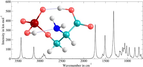
3.3. Application to Deprotonated Phosphoserine
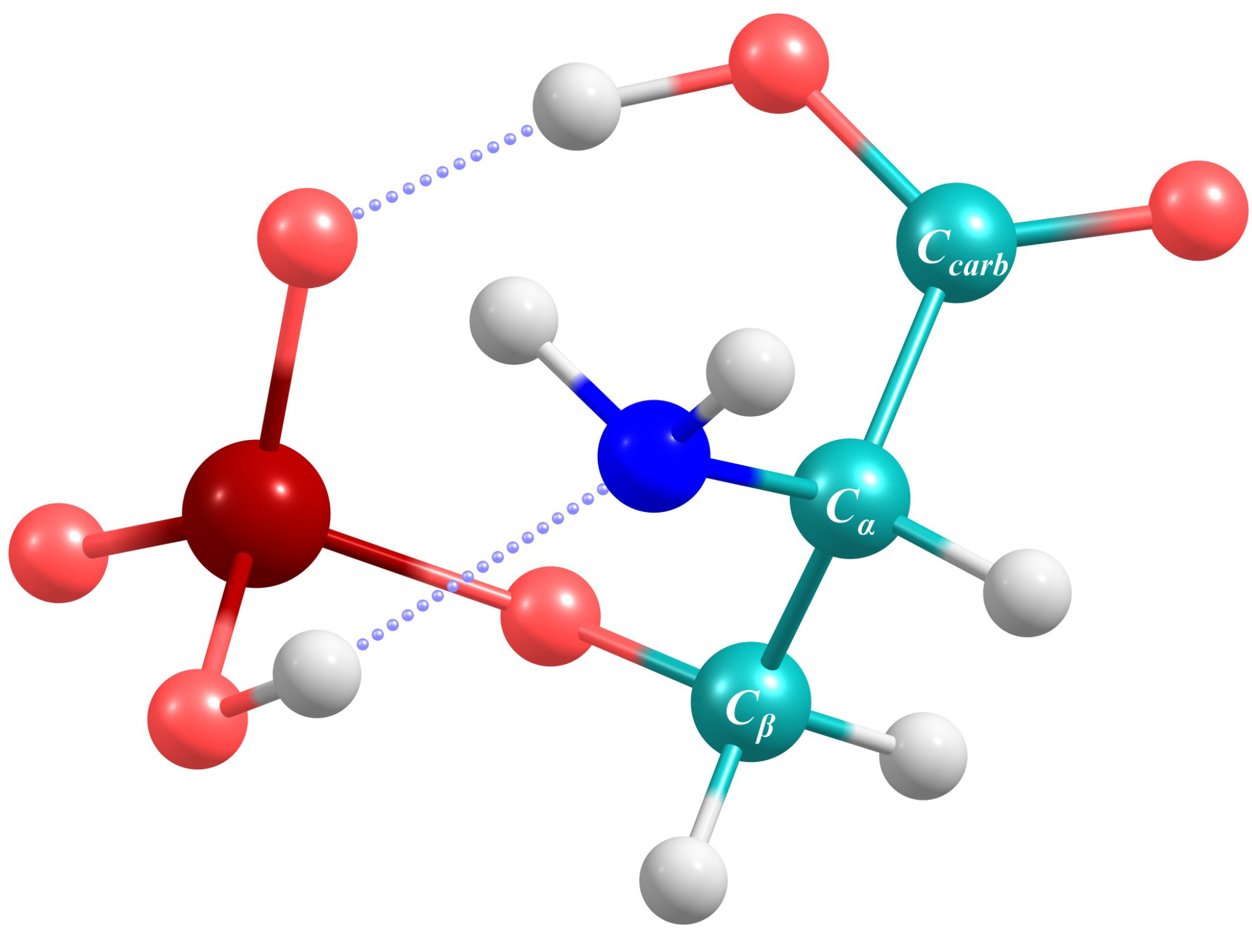
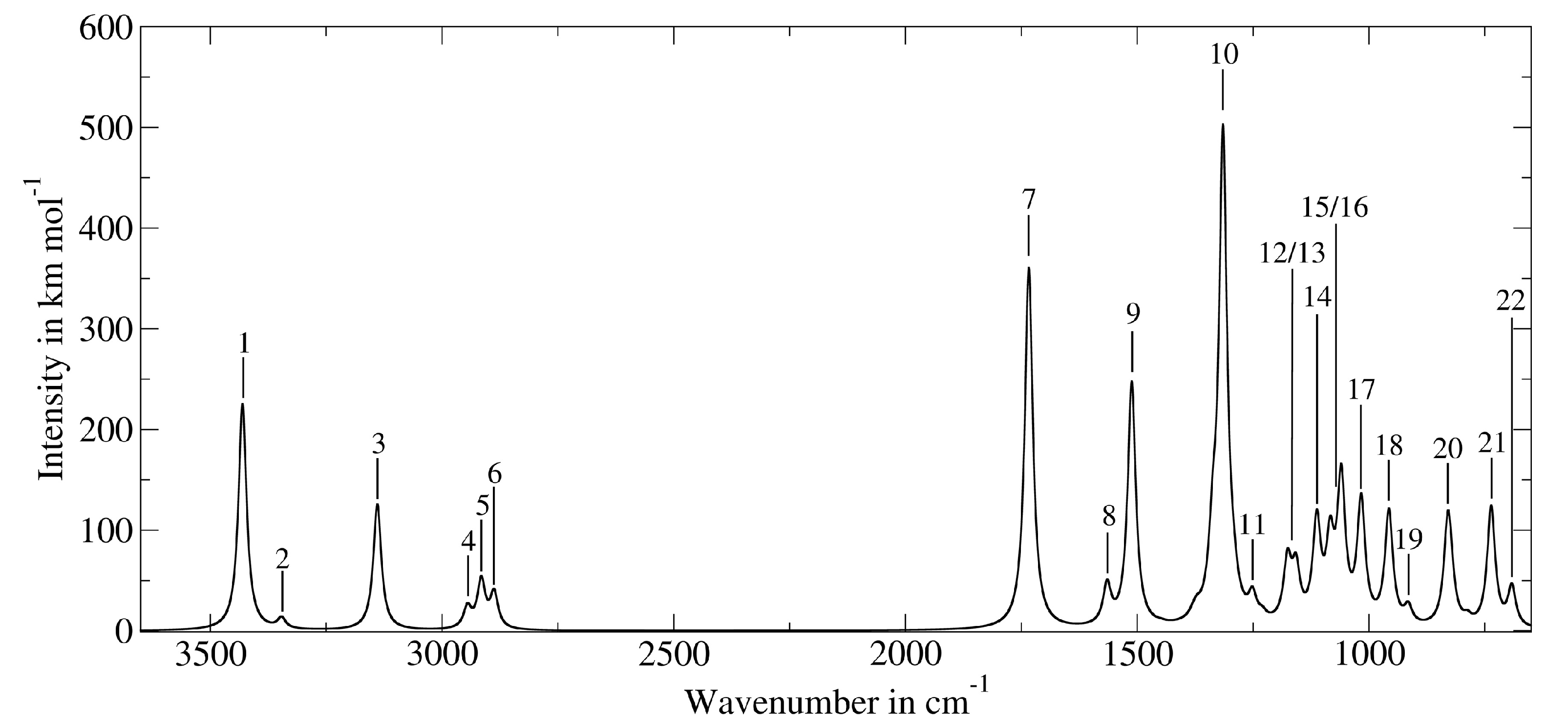
| Band Number | PT2-VSCF (cm−1) | Intensity (km mol−1) | IRMPD (cm−1) [118] | Main Contributions |
|---|---|---|---|---|
| 1 | 3430 | 225 | n.o. | νOH |
| 2 | 3346 | 11 | n.o. | νNH2,as |
| 3 | 3139 | 125 | n.o. | νNH2,s |
| 4 | 2945 | 21 | n.o. | νCαH |
| 5 | 2915 | 47 | n.o. | νCβH2,s |
| 6 | 2888 | 35 | n.o. | νCβH2,as |
| 7 | 1734 | 359 | 1728 | νCcarb =O |
| 8 | 1565 | 39 | 1610 | δNH2 |
| 9 | 1512 | 244 | 1461 | δCcarbOH,ip |
| 1449 | 1 | 1419 | δCβH2 | |
| 1380 | 4 | n.o. | τNH2 and δNCαH | |
| 1371 | 9 | n.o. | ωCβH2 | |
| 1337 | 68 | n.o. | νCcarb −O and τCβH2 | |
| 10 | 1315 | 484 | 1291 | νP =O |
| 1292 | 21 | n.o. | ωCβH2 and δCcarbCαH and νCcarb −O | |
| 11 | 1251 | 24 | n.o. | νCα − Cβ and δCβCαH and νCα −N and τNH2 |
| 1230 | 6 | n.o. | νCcarbCα and δCcarbCαH and τNH2 | |
| 12 | 1176 | 60 | n.o. | δCcarbOH,oop |
| 13 | 1157 | 51 | n.o. | νCβO |
| 14 | 1113 | 99 | 1108 | δPOH |
| 15 | 1084 | 74 | n.o. | νNCαCcarb,as and νCβO |
| 16 | 1060 | 141 | 1052 | ωNH2 |
| 17 | 1017 | 121 | 1028 | νP − O H −bonded |
| 18 | 957 | 113 | n.o. | νNCαCβ,as |
| 19 | 915 | 17 | n.o. | νNCαCβ,s and νNCαCcarb,as and νCcarbCαCβ,as |
| 20 | 830 | 98 | 836 | νP −OH |
| 823 | 24 | 812 | δCcarbCαCβ and δCcarbO2,oop | |
| 787 | 7 | n.o. | δCcarbO2 and δCcarbCαCβ | |
| 21 | 736 | 120 | 738 | νP −OCβ and δCcarbO2 |
| 22 | 692 | 39 | n.o. | δCαNCβCcarb,umbrella and νP − OCbeta |
| 513 | 41 | n.o. | δPOH,oop |
4. Conclusions
Author Contributions
Conflicts of Interest
References
- Scott, A.P.; Radom, L. Harmonic Vibrational Frequencies: An Evaluation of Hartree-Fock, Møller-Plesset, Quadratic Configuration Interaction, Density Functional Theory, and Semiempirical Scale Factors. J. Phys. Chem. 1996, 100, 16502–16513. [Google Scholar]
- Sinha, P.; Boesch, S.E.; Gu, C.; Wheeler, R.A.; Wilson, A.K. Harmonic Vibrational Frequencies: Scaling Factors for HF, B3LYP, and MP2 Methods in Combination with Correlation Consistent Basis Sets. J. Phys. Chem. A 2004, 108, 9213–9217. [Google Scholar] [CrossRef]
- Bowman, J.M. Self-Consistent Field Energies and Wavefunctions for Coupled Oscillators. J. Chem. Phys. 1978, 68, 608–610. [Google Scholar] [CrossRef]
- Cohen, M.; Greita, S.; McEarchran, R. Approximate and Exact Quantum Mechanical Energies and Eigenfunctions for a System of Coupled Oscillators. Chem. Phys. Lett. 1979, 60, 445–450. [Google Scholar] [CrossRef]
- Gerber, R.; Ratner, M. A Semiclassical Self-Consistent Field (SC SCF) Approximation for Eigenvalues of Coupled-Vibration Systems. Chem. Phys. Lett. 1979, 68, 195–198. [Google Scholar]
- Bowman, J.M. The Self-Consistent-Field Approach to Polyatomic Vibrations. Acc. Chem. Res. 1986, 19, 202–208. [Google Scholar] [CrossRef]
- Carter, S.; Culik, S.J.; Bowman, J.M. Vibrational Self-Consistent Field Method for Many-Mode Systems: A New Approach and Application to the Vibrations of CO Adsorbed on Cu(100). J. Chem. Phys. 1997, 107, 10458–10469. [Google Scholar] [CrossRef]
- Carney, G.D.; Sprandel, L.L.; Kern, C.W. Variational Approaches to Vibration-Rotation Spectroscopy for Polyatomic Molecules. In Advances in Chemical Physics; Prigogine, I., Rice, S.A., Eds.; John Wiley & Sons,Inc.: Hoboken, NJ, USA, 2007; Volume 37, pp. 305–379. [Google Scholar]
- Barone, V. Vibrational Zero-Point Energies and Thermodynamic Functions Beyond the Harmonic Approximation. J. Chem. Phys. 2004, 120, 3059–3065. [Google Scholar] [CrossRef] [PubMed]
- Barone, V. Anharmonic Vibrational Properties by a Fully Automated Second-order Perturbative Approach. J. Chem. Phys. 2005, 122. [Google Scholar] [CrossRef]
- Frisch, M.J.; Trucks, G.W.; Schlegel, H.B.; Scuseria, G.E.; Robb, M.A.; Cheeseman, J.R.; Scalmani, G.; Barone, V.; Mennucci, B.; Petersson, G.A.; et al. Gaussian 09, Revision D.01; Gaussian Inc.: Wallingford, CT, USA, 2013.
- Barone, V.; Biczysko, M.; Bloino, J. Fully Anharmonic IR and Raman Spectra of Medium-Size Molecular Systems: Accuracy and Interpretation. Phys. Chem. Chem. Phys. 2014, 16, 1759–1787. [Google Scholar] [CrossRef] [PubMed]
- Biczysko, M.; Bloino, J.; Carnimeo, I.; Panek, P.; Barone, V. Fully Ab Initio IR Spectra for Complex Molecular Systems from Perturbative Vibrational Approaches: Glycine as a Test Case. J. Mol. Struct. 2012, 1009, 74–82. [Google Scholar] [CrossRef]
- Chaban, G.M.; Jung, J.O.; Gerber, R.B. Ab Initio Calculation of Anharmonic Vibrational States of Polyatomic Systems: Electronic Structure Combined with Vibrational Self-Consistent Field. J. Chem. Phys. 1999, 111, 1823–1829. [Google Scholar] [CrossRef]
- Jung, J.O.; Gerber, R.B. Vibrational Wave Functions and Spectroscopy of (H2O)n, n = 2, 3, 4, 5: Vibrational Self-Consistent Field with Correlation Corrections. J. Chem. Phys. 1996, 105, 10332–10348. [Google Scholar] [CrossRef]
- Chaban, G.M.; Jung, J.O.; Gerber, R.B. Anharmonic Vibrational Spectroscopy of Hydrogen-Bonded Systems Directly Computed from Ab Initio Potential Surfaces: (H2O)n, n = 2, 3; Cl−(H2O)n, n = 1, 2; H+(H2O)n, n = 1, 2; H2O-CH3OH. J. Phys. Chem. A 2000, 104, 2772–2779. [Google Scholar] [CrossRef]
- Chaban, G.M.; Jung, J.O.; Gerber, R.B. Anharmonic Vibrational Spectroscopy of Glycine: Testing of Ab Initio and Empirical Potentials. J. Phys. Chem. A 2000, 104, 10035–10044. [Google Scholar] [CrossRef]
- Miller, Y.; Chaban, G.; Gerber, R. Theoretical Study of Anharmonic Vibrational Spectra of HNO3, HNO3-H2O, HNO4: Fundamental, Overtone and Combination Excitations. Chem. Phys. 2005, 313, 213–224. [Google Scholar] [CrossRef]
- Roy, T.K.; Carrington, T.; Gerber, R.B. Approximate First-Principles Anharmonic Calculations of Polyatomic Spectra Using MP2 and B3LYP Potentials: Comparisons with Experiment. J. Phys. Chem. A 2014, 118, 6730–6739. [Google Scholar] [CrossRef] [PubMed]
- Schmidt, M.W.; Baldridge, K.K.; Boatz, J.A.; Elbert, S.T.; Gordon, M.S.; Jensen, J.H.; Koseki, S.; Matsunaga, N.; Nguyen, K.A.; Su, S.; et al. General Atomic and Molecular Electronic Structure System. J. Comput. Chem. 1993, 14, 1347–1363. [Google Scholar] [CrossRef]
- Valiev, M.; Bylaska, E.; Govind, N.; Kowalski, K.; Straatsma, T.; Dam, H.V.; Wang, D.; Nieplocha, J.; Apra, E.; Windus, T.; et al. NWChem: A Comprehensive and Scalable Open-Source Solution for Large Scale Molecular Simulations. Comput. Phys. Commun. 2010, 181, 1477–1489. [Google Scholar] [CrossRef]
- Werner, H.; Knowles, P.J.; Knizia, G.; Manby, F.R.; Schütz, M.; Celani, P.; Korona, T.; Lindh, R.; Mitrushenkov, A.; Rauhut, G.; et al. MOLPRO, Version 2012.1, A Package of Ab Initio Programs. 2012. Available online: http://www.molpro.net/ (accessed on 15 December 2014).
- Møller, C.; Plesset, M.S. Note on an Approximation Treatment for Many-Electron Systems. Phys. Rev. 1934, 46, 618–622. [Google Scholar] [CrossRef]
- Fletcher, G.D.; Schmidt, M.W.; Gordon, M.S. Developments in Parallel Electronic Structure Theory. In Advances in Chemical Physics; Prigogine, I., Rice, S.A., Eds.; John Wiley & Sons, Inc.: Hoboken, NJ, USA, 2007; Volume 110, pp. 267–294. [Google Scholar]
- Aikens, C.M.; Gordon, M.S. Parallel Unrestricted MP2 Analytic Gradients Using the Distributed Data Interface. J. Phys. Chem. A 2004, 108, 3103–3110. [Google Scholar] [CrossRef]
- Sachs, E.S.; Hinze, J.; Sabelli, N.H. Frozen Core Approximation, a Pseudopotential Method Tested on Six States of NaH. J. Chem. Phys. 1975, 62, 3393–3398. [Google Scholar] [CrossRef]
- Dunning, T.H. Gaussian Basis Sets for Use in Correlated Molecular Calculations. I. The Atoms Boron Through Neon and Hydrogen. J. Chem. Phys. 1989, 90, 1007–1023. [Google Scholar] [CrossRef]
- Bowman, J.M.; Carrington, T.; Meyer, H.D. Variational Quantum Approaches for Computing Vibrational Energies of Polyatomic Molecules. Mol. Phys. 2008, 106, 2145–2182. [Google Scholar] [CrossRef]
- Chan, M.; Carrington, T.; Manzhos, S. Anharmonic Vibrations of the Carboxyl Group in Acetic Acid on TiO2: Implications For Adsorption Mode Assignment in Dye-Sensitized Solar Cells. Phys. Chem. Chem. Phys. 2013, 15, 10028–10034. [Google Scholar] [CrossRef] [PubMed]
- Sakurai, J.J.; Tuan, S.F. Modern Quantum Mechanics; Addison-Wesley: Boston, MA, USA, 1985; Volume 1. [Google Scholar]
- Griffiths, D.J.; Harris, E.G. Introduction to Quantum Mechanics; Prentice Hall: Upper Saddle River, NJ, USA, 1995; Volume 2. [Google Scholar]
- Ratner, M.A.; Gerber, R.B. Excited Vibrational States of Polyatomic Molecules: The Semiclassical Self-Consistent Field Approach. J. Phys. Chem. 1986, 90, 20–30. [Google Scholar] [CrossRef]
- Watson, J.K. Simplification of the Molecular Vibration-Rotation Hamiltonian. Mol. Phys. 1968, 15, 479–490. [Google Scholar] [CrossRef]
- Bowman, J.M.; Carter, S.; Huang, X. MULTIMODE: A Code to Calculate Rovibrational Energies of Polyatomic Molecules. Int. Rev. Phys. Chem. 2003, 22, 533–549. [Google Scholar] [CrossRef]
- Roy, T.K.; Gerber, R.B. Vibrational Self-Consistent Field Calculations for Spectroscopy of Biological Molecules: New Algorithmic Developments and Applications. Phys. Chem. Chem. Phys. 2013, 15, 9468–9492. [Google Scholar] [CrossRef] [PubMed]
- Gregurick, S.K.; Fredj, E.; Elber, R.; Gerber, R.B. Vibrational Spectroscopy of Peptides and Peptide-Water Complexes: Anharmonic Coupled-Mode Calculations. J. Phys. Chem. B 1997, 101, 8595–8606. [Google Scholar] [CrossRef]
- Gregurick, S.K.; Liu, J.H.Y.; Brant, D.A.; Gerber, R.B. Anharmonic Vibrational Self-Consistent Field Calculations as an Approach to Improving Force Fields for Monosaccharides. J. Phys. Chem. B 1999, 103, 3476–3488. [Google Scholar] [CrossRef]
- Kowal, A.T. First-principles Calculation of Geometry and Anharmonic Vibrational Spectra of Thioformamide and Thioformamide-d2. J. Chem. Phys. 2006, 124. [Google Scholar] [CrossRef]
- Carter, S.; Bowman, J.M.; Handy, N.C. Extensions and Tests of MULTIMODE: A Code to Obtain Accurate Vibration/Rotation Energies of Many-Mode Molecules. Theor. Chem. Acc. 1998, 100, 191–198. [Google Scholar]
- Rheinecker, J.; Bowman, J.M. The Calculated Infrared Spectrum of Cl H2O Using a New Full Dimensional Ab Initio Potential Surface and Dipole Moment Surface. J. Chem. Phys. 2006, 125. [Google Scholar] [CrossRef]
- Norris, L.S.; Ratner, M.A.; Roitberg, A.E.; Gerber, R.B. Møller-Plesset Perturbation Theory Applied to Vibrational Problems. J. Chem. Phys. 1996, 105, 11261–11267. [Google Scholar] [CrossRef]
- Pele, L.; Gerber, R.B. On the Number of Significant Mode-Mode Anharmonic Couplings in Vibrational Calculations: Correlation-Corrected Vibrational Self-Consistent Field Treatment of Di-, Tri-, and Tetrapeptides. J. Chem. Phys. 2008, 128. [Google Scholar] [CrossRef]
- Pele, L.; Brauer, B.; Gerber, R. Acceleration of Correlation-Corrected Vibrational Self-Consistent Field Calculation Times for Large Polyatomic Molecules. Theor. Chem. Acc. 2007, 117, 69–72. [Google Scholar] [CrossRef]
- Matsunaga, N.; Chaban, G.M.; Gerber, R.B. Degenerate Perturbation Theory Corrections for the Vibrational Self-Consistent Field Approximation: Method and Applications. J. Chem. Phys. 2002, 117, 3541–3547. [Google Scholar]
- Bowman, J.M.; Christoffel, K.; Tobin, F. Application of SCF-SI Theory to Vibrational Motion in Polyatomic Molecules. J. Phys. Chem. 1979, 83, 905–912. [Google Scholar] [CrossRef]
- Christoffel, K.M.; Bowman, J.M. Investigations of Self-Consistent Field, SCF CI and Virtual Stateconfiguration Interaction Vibrational Energies for a Model Three-Mode System. Chem. Phys. Lett. 1982, 85, 220–224. [Google Scholar] [CrossRef]
- Christiansen, O.; Luis, J.M. Beyond Vibrational Self-Consistent-Field Methods: Benchmark Calculations for the Fundamental Vibrations of Ethylene. Int. J. Quantum Chem. 2005, 104, 667–680. [Google Scholar] [CrossRef]
- Neff, M.; Rauhut, G. Toward Large Scale Vibrational Configuration Interaction Calculations. J. Chem. Phys. 2009, 131. [Google Scholar] [CrossRef] [PubMed]
- Kaulfuss, U.B.; Altenbokum, M. Anharmonic Oscillator as a Test of the Coupled-Cluster Method. Phys. Rev. D 1986, 33, 3658–3664. [Google Scholar] [CrossRef]
- Nagalakshmi, V.; Lakshminarayana, V.; Sumithra, G.; Prasad, M.D. Coupled Cluster Description of Anharmonic Molecular Vibrations. Application to O3 and SO2. Chem. Phys. Lett. 1994, 217, 279–282. [Google Scholar] [CrossRef]
- Thomsen, B.; Yagi, K.; Christiansen, O. Optimized Coordinates in Vibrational Coupled Cluster Calculations. J. Chem. Phys. 2014, 140. [Google Scholar] [CrossRef]
- Culot, F.; Liévin, J. A Multiconfigurational SCF Computational Method for the Resolution of the Vibrational Schrödinger Equation in Polyatomic Molecules. Theor. Chim. Acta 1994, 89, 227–250. [Google Scholar] [CrossRef]
- Meyer, H.D. Studying Molecular Quantum Dynamics With the Multiconfiguration Time-Dependent Hartree Method. Wiley Interdiscip. Rev.: Comput. Mol. Sci. 2012, 2, 351–374. [Google Scholar] [CrossRef]
- Njegic, B.; Gordon, M.S. Exploring the Effect of Anharmonicity of Molecular Vibrations on Thermodynamic Properties. J. Chem. Phys. 2006, 125. [Google Scholar] [CrossRef]
- Bounouar, M.; Scheurer, C. The Impact of Approximate VSCF Schemes and Curvilinear Coordinates on the Anharmonic Vibrational Frequencies of Formamide and Thioformamide. Chem. Phys. 2008, 347, 194–207. [Google Scholar]
- Strobusch, D.; Scheurer, C. Hierarchical Expansion of the Kinetic Energy Operator in Curvilinear Coordinates for the Vibrational Self-Consistent Field Method. J. Chem. Phys. 2011, 135. [Google Scholar] [CrossRef]
- Boatz, J.A.; Gordon, M.S. Decomposition of Normal-Coordinate Vibrational Frequencies. J. Phys. Chem. 1989, 93, 1819–1826. [Google Scholar] [CrossRef]
- Yagi, K.; Hirao, K.; Taketsugu, T.; Schmidt, M.W.; Gordon, M.S. Ab Initio Vibrational State Calculations with a Quartic Force Field: Applications to H2CO, C2H4, CH3OH, CH3CCH and C6H6. J. Chem. Phys. 2004, 121, 1383–1389. [Google Scholar] [CrossRef] [PubMed]
- Shimanouchi, T. Tables of Molecular Vibrational Frequencies Consolidated Volume I. Natl. Bur. Stand. 1972, 1, 1–164. [Google Scholar]
- Herzberg, G. Infrared and Raman Spectra of Polyatomic Molecules; Van Nostrand: New York, NY, USA, 1949. [Google Scholar]
- Smith, L.G. The Infra-Red Spectrum of C2H6. J. Chem. Phys. 1949, 17, 139–167. [Google Scholar] [CrossRef]
- Weiss, S.; Leroi, G.E. Direct Observation of the Infrared Torsional Spectrum of C2H6, CH3CD3, and C2D6. J. Chem. Phys. 1968, 48, 962–967. [Google Scholar] [CrossRef]
- Lutz, O.M.; Rode, B.M.; Bonn, G.K.; Huck, C.W. The Impact of Highly Correlated Potential Energy Surfaces on the Anharmonically Corrected IR Spectrum of Acetonitrile. Spectrochim. Acta Part A 2014, 131, 545–555. [Google Scholar] [CrossRef]
- Bartlett, R.J.; Purvis, G.D. Many-Body Perturbation Theory, Coupled-Pair Many-Electron Theory, and the Importance of Quadruple Excitations for the Correlation Problem. Int. J. Quantum Chem. 1978, 14, 561–581. [Google Scholar] [CrossRef]
- Pople, J.A.; Krishnan, R.; Schlegel, H.B.; Binkley, J.S. Electron Correlation Theories and Their Application to the Study of Simple Reaction Potential Surfaces. Int. J. Quantum Chem. 1978, 14, 545–560. [Google Scholar] [CrossRef]
- Gauss, J.; Stanton, J.F. Perturbative Treatment of Triple Excitations in Coupled-cluster Calculations of Nuclear Magnetic Shielding Constants. J. Chem. Phys. 1996, 104, 2574–2583. [Google Scholar] [CrossRef]
- Pople, J.A.; Head-Gordon, M.; Raghavachari, K. Quadratic Configuration Interaction. A General Technique for Determining Electron Correlation Energies. J. Chem. Phys. 1987, 87, 5968–5975. [Google Scholar] [CrossRef]
- Piecuch, P.; Włoch, M. Renormalized Coupled-Cluster Methods Exploiting Left Eigenstates of the Similarity-Transformed Hamiltonian. J. Chem. Phys. 2005, 123. [Google Scholar] [CrossRef]
- Piecuch, P.; Włoch, M.; Gour, J.R.; Kinal, A. Single-Reference, Size-Extensive, Non-Iterative Coupled-Cluster Approaches to Bond Breaking and Biradicals. Chem. Phys. Lett. 2006, 418, 467–474. [Google Scholar] [CrossRef]
- Dennison, D.M. The Infrared Spectra of Polyatomic Molecules Part I. Rev. Mod. Phys. 1931, 3, 280–345. [Google Scholar] [CrossRef]
- Barker, E.F.; Sleator, W.W. The Infrared Spectrum of Heavy Water. J. Chem. Phys. 1935, 3, 660–663. [Google Scholar] [CrossRef]
- Benedict, W.S.; Gailar, N.; Plyler, E.K. Rotation-Vibration Spectra of Deuterated Water Vapor. J. Chem. Phys. 1956, 24, 1139–1165. [Google Scholar] [CrossRef]
- Amat, G.; Pimbert, M. On Fermi Resonance in Carbon Dioxide. J. Mol. Spectrosc. 1965, 16, 278–290. [Google Scholar] [CrossRef]
- Suzuki, I. General Anharmonic Force Constants of Carbon Dioxide. J. Mol. Spectrosc. 1968, 25, 479–500. [Google Scholar] [CrossRef]
- Davidson, D.W.; Stoicheff, B.P.; Bernstein, H.J. The Infrared and Raman Spectra of Formaldehyde-d1 Vapor. J. Chem. Phys. 1954, 22, 289–294. [Google Scholar] [CrossRef]
- Blau, H.H.; Nielsen, H.H. The Infrared Absorption Spectrum of Formaldehyde Vapor. J. Mol. Spectrosc. 1957, 1, 124–132. [Google Scholar] [CrossRef]
- Nakagawa, T.; Kashiwagi, H.; Kurihara, H.; Morino, Y. Vibration-Rotation Spectra of Formaldehyde: Band Contour Analysis of the ν2 and ν3 Fundamentals. J. Mol. Spectrosc. 1969, 31, 436–450. [Google Scholar] [CrossRef]
- Lafferty, W.J.; Thibault, R.J. High Resolution Infrared Spectra of H2, C12C13H2, and H2. J. Mol. Spectrosc. 1964, 14, 79–96. [Google Scholar] [CrossRef]
- Scott, J.; Rao, K. Infrared Absorption Bands of Acetylene: Part I. Analysis of the Bands at 13.7µ. J. Mol. Spectrosc. 1965, 16, 15–23. [Google Scholar] [CrossRef]
- Scott, J.; Rao, K.N. Infrared Absorption Bands of Acetylene: Part III. Analysis of the Bands at 3µ. J. Mol. Spectrosc. 1966, 20, 438–460. [Google Scholar] [CrossRef]
- Williams, V.Z. Infra-Red Spectra of Monomeric Formic Acid and Its Deuterated Forms. I. High Frequency Region. J. Chem. Phys. 1947, 15, 232–242. [Google Scholar] [CrossRef]
- Wilmshurst, J.K. Vibrational Assignment in Monomeric Formic Acid. J. Chem. Phys. 1956, 25, 478–480. [Google Scholar] [CrossRef]
- Millikan, R.C.; Pitzer, K.S. Infrared Spectra and Vibrational Assignment of Monomeric Formic Acid. J. Chem. Phys. 1957, 27, 1305–1308. [Google Scholar] [CrossRef]
- Miyazawa, T.; Pitzer, K.S. Internal Rotation and Infrared Spectra of Formic Acid Monomer and Normal Coordinate Treatment of Out-Of-Plane Vibrations of Monomer, Dimer, and Polymer. J. Chem. Phys. 1959, 30, 1076–1086. [Google Scholar] [CrossRef]
- Allen, H.C.; Plyler, E.K. ν3 Band of Methane. J. Chem. Phys. 1957, 26, 972–973. [Google Scholar] [CrossRef]
- Herranz, J.; Morcillo, J.; Gómez, A. The ν2 Infrared Band of CH4 and CD4. J. Mol. Spectrosc. 1966, 19, 266–282. [Google Scholar] [CrossRef]
- King, W.T.; Mills, I.M.; Crawford, B. Normal Coordinates in the Methyl Halides. J. Chem. Phys. 1957, 27, 455–457. [Google Scholar] [CrossRef]
- Jones, E.; Popplewell, R.; Thompson, H. Vibration—Rotation Bands of Methyl Chloride. Spectrochim. Acta 1966, 22, 669–680. [Google Scholar]
- Maki, A.G.; Thibault, R. Analysis of Some Perturbations in the ν4 Band of Methyl Chloride. J. Chem. Phys. 1968, 48, 2163–2167. [Google Scholar] [CrossRef]
- Morillon-Chapey, M.; Graner, G. Fine Structure in the ν1 Band of CH3Cl near 2970 cm−1. J. Mol. Spectrosc. 1969, 31, 155–169. [Google Scholar] [CrossRef]
- Tanaka, C.; Kuratani, K.; Mizushima, S.I. In-Plane Normal Vibrations of Methanol. Spectrochim. Acta 1957, 9, 265–269. [Google Scholar] [CrossRef]
- Van Thiel, M.; Becker, E.D.; Pimentel, G.C. Infrared Studies of Hydrogen Bonding of Methanol by the Matrix Isolation Technique. J. Chem. Phys. 1957, 27, 95–99. [Google Scholar] [CrossRef]
- Falk, M.; Whalley, E. Infrared Spectra of Methanol and Deuterated Methanols in Gas, Liquid, and Solid Phases. J. Chem. Phys. 1961, 34, 1554–1568. [Google Scholar] [CrossRef]
- Nakagawa, I.; Shimanouchi, T. Rotation-Vibration Spectra and Rotational, Coriolis Coupling, Centrifugal Distortion and Potential Constants of Methyl Cyanide. Spectrochim. Acta 1962, 18, 513–539. [Google Scholar] [CrossRef]
- Tolonen, A.; Koivusaari, M.; Paso, R.; Schroderus, J.; Alanko, S.; Anttila, R. The Infrared Spectrum of Methyl Cyanide Between 850 and 1150 cm−1: Analysis of the ν4, ν7, and 3ν18 Bands with Resonances. J. Mol. Spectrosc. 1993, 160, 554–565. [Google Scholar] [CrossRef]
- Venkateswarlu, P. The Rotation-Vibration Spectrum of Methyl Cyanide in the Region 1.6 µ–20 µ. J. Chem. Phys. 1951, 19, 293–298. [Google Scholar] [CrossRef]
- Venkateswarlu, P. The Infrared Spectrum of Methyl Cyanide. J. Chem. Phys. 1952, 20, 923–923. [Google Scholar] [CrossRef]
- Thompson, H.W.; Williams, R.L. The Infra-red Spectra of Methyl Cyanide and Methyl Isocyanide. Trans. Faraday Soc. 1952, 48, 502–513. [Google Scholar]
- Parker, F.; Nielsen, A.; Fletcher, W. The Infrared Absorption Spectrum of Methyl Cyanide Vapor. J. Mol. Spectrosc. 1957, 1, 107–123. [Google Scholar] [CrossRef]
- Huet, T. The ν1 and ν5 Fundamental Bands of Methyl Cyanide. J. Mol. Struct. 2000, 517, 127–131. [Google Scholar] [CrossRef]
- Arnett, R.L.; Crawford, B.L. The Vibrational Frequencies of Ethylene. J. Chem. Phys. 1950, 18, 118–126. [Google Scholar] [CrossRef]
- Allen, H.C.; Plyler, E.K. The Structure of Ethylene from Infrared Spectra. J. Am. Chem. Soc. 1958, 80, 2673–2676. [Google Scholar]
- Lord, R.C.; Nolin, B. Vibrational Spectra of Ethylene Oxide and Ethylene Oxide-d4. J. Chem. Phys. 1956, 24, 656–658. [Google Scholar]
- Potts, W. The Fundamental Vibration Frequencies of Ethylene Oxide and Ethylene Imine. Spectrochim. Acta 1965, 21, 511–527. [Google Scholar] [CrossRef]
- Kirby-Smith, J.S.; Bonner, L.G. The Raman Spectra of Gaseous Substances 1. Apparatus and the Spectrum of Methylamine. J. Chem. Phys. 1939, 7, 880–883. [Google Scholar] [CrossRef]
- Gray, A.P.; Lord, R.C. Rotation-Vibration Spectra of Methyl Amine and Its Deuterium Derivatives. J. Chem. Phys. 1957, 26, 690–705. [Google Scholar] [CrossRef]
- Tsuboi, M.; Hirakawa, A.Y.; Ino, T.; Sasaki, T.; Tamagake, K. Amino Wagging and Inversion in Methylamines. J. Chem. Phys. 1964, 41, 2721–2734. [Google Scholar] [CrossRef]
- Cole, A.; Lafferty, W.; Thibault, R. Rotational Fine Structure of the Perpendicular Band, ν7, of Ethane. J. Mol. Spectrosc. 1969, 29, 365–374. [Google Scholar] [CrossRef]
- Nakagawa, I.; Shimanouchi, T. Rotation-Vibration Spectra and Rotational, Coriolis Coupling and Potential Constants of Ethane, Ethane-d6 and Ethane-1, 1, 1-d3. J. Mol. Spectrosc. 1971, 39, 255–274. [Google Scholar] [CrossRef]
- Taylor, R.C.; Vidale, G.L. Raman Spectrum and Vibrational Assignments of Gaseous Dimethyl Ether. J. Chem. Phys. 1957, 26, 122–123. [Google Scholar] [CrossRef]
- Fateley, W.; Miller, F.A. Torsional Frequencies in the Far Infrared-II: Molecules With Two or Three Methyl Rotors. Spectrochim. Acta 1962, 18, 977–993. [Google Scholar]
- Stepanian, S.G.; Reva, I.D.; Radchenko, E.D.; Rosado, M.T.S.; Duarte, M.L.T.S.; Fausto, R.; Adamowicz, L. Matrix-Isolation Infrared and Theoretical Studies of the Glycine Conformers. J. Phys. Chem. A 1998, 102, 1041–1054. [Google Scholar] [CrossRef]
- Brauer, B.; Chaban, G.M.; Gerber, R.B. Spectroscopically-Tested, Improved, Semi-Empirical Potentials for Biological Molecules: Calculations for Glycine, Alanine and Proline. Phys. Chem. Chem. Phys. 2004, 6, 2543–2556. [Google Scholar] [CrossRef]
- Goulden, C. Methods of Statistical Analysis; Wiley: New York, NY, USA, 2007; pp. 50–55. [Google Scholar]
- Kataoka, H.; Nakai, K.; Katagiri, Y.; Makita, M. Analysis of Free and Bound O-Phosphoamino Acids in Urine by Gas Chromatography with Flame Photometric Detection. Biomed. Chromatogr. 1993, 7, 184–188. [Google Scholar] [CrossRef] [PubMed]
- Mason, R.; Trumbore, M.W.; Pettegrew, J.W. Membrane Interactions of a Phosphomonoester Elevated Early in Alzheimer’s Disease. Neurobiol. Aging 1995, 16, 531–539. [Google Scholar] [CrossRef] [PubMed]
- Chiarla, C.; Giovannini, I.; Siegel, J.H. High Phosphoserine in Sepsis: Panel of Clinical and Plasma Amino Acid Correlations. SpringerPlus 2014, 3. [Google Scholar] [CrossRef] [PubMed]
- Scuderi, D.; Correia, C.F.; Balaj, O.P.; Ohanessian, G.; Lemaire, J.; Maitre, P. Structural Characterization by IRMPD Spectroscopy and DFT Calculations of Deprotonated Phosphorylated Amino Acids in the Gas Phase. ChemPhysChem 2009, 10, 1630–1641. [Google Scholar] [CrossRef] [PubMed]
- Sample Availability: Not available.
© 2014 by the authors. Licensee MDPI, Basel, Switzerland. This article is an open access article distributed under the terms and conditions of the Creative Commons Attribution license ( http://creativecommons.org/licenses/by/4.0/).
Share and Cite
Lutz, O.M.D.; Rode, B.M.; Bonn, G.K.; Huck, C.W. Largely Reduced Grid Densities in a Vibrational Self-Consistent Field Treatment Do Not Significantly Impact the ResultingWavenumbers. Molecules 2014, 19, 21253-21275. https://doi.org/10.3390/molecules191221253
Lutz OMD, Rode BM, Bonn GK, Huck CW. Largely Reduced Grid Densities in a Vibrational Self-Consistent Field Treatment Do Not Significantly Impact the ResultingWavenumbers. Molecules. 2014; 19(12):21253-21275. https://doi.org/10.3390/molecules191221253
Chicago/Turabian StyleLutz, Oliver M. D., Bernd M. Rode, Günther K. Bonn, and Christian W. Huck. 2014. "Largely Reduced Grid Densities in a Vibrational Self-Consistent Field Treatment Do Not Significantly Impact the ResultingWavenumbers" Molecules 19, no. 12: 21253-21275. https://doi.org/10.3390/molecules191221253
APA StyleLutz, O. M. D., Rode, B. M., Bonn, G. K., & Huck, C. W. (2014). Largely Reduced Grid Densities in a Vibrational Self-Consistent Field Treatment Do Not Significantly Impact the ResultingWavenumbers. Molecules, 19(12), 21253-21275. https://doi.org/10.3390/molecules191221253