1. Introduction
The propagation of epidemic diseases within a host population has been studied since several decades ago. Kermack and McKendrick developed one of the first works in the subject [
1]. They proposed an SIR epidemic model where the host population is split in three categories depending on the status of the individuals with respect to the disease. In such a context,
S,
I, and
R denote, respectively, the susceptible, infectious, and recovered subpopulations. Later, a lot of models have been proposed and analysed in the specialised literature. Such models consider some additional population categories and/or control actions for eradicating or, at least, diminishing the effects of the disease in the host population [
2,
3,
4,
5]. In this sense, the models can include the exposed subpopulation
E composed by individuals without symptoms of the disease and without the capacity of transmitting the infection to a susceptible individual after a contagion. Such a model is referred to as the SEIR model [
6]. The more usual control actions are the vaccination of susceptible individuals and the treatment of infectious individuals by antivirals, antibiotics, or other medicaments [
7,
8]. Additionally, other control actions such as quarantine of infectious individuals have also been proposed [
9]. These control actions give place to include other subpopulations in the models as vaccinated, treated, and quarantined ones [
10,
11,
12,
13]. For instance, the authors in [
13] propose a SVEIR model to analyse the impact of vaccination in the control of spread of poliomyelitis. Moreover, the control actions can be applied in continuous-time or impulsive ways during the vaccination campaigns and/or treatment procedures [
14,
15,
16]. The social distancing is another alternative way to fight against the propagation of infectious diseases [
17]. Such a measure may be crucial when there are asymptomatic infectious individuals and/or neither vaccines nor medicaments are available to maintain the disease propagation under control. The early phase of the COVID-19 pandemic is a clear example of such a fact [
18]. In such situations, the susceptible subpopulation can be split in several categories according to its preventive care and responsible behaviour to avoid the disease contagion. For instance, the study in [
19] considers two susceptible subpopulations according to its risk aversion. One of the categories contains individuals with self-protection awareness, and the other one is composed by people without such an awareness. Recently, new approaches from game theory have been proposed for analysing the spreading of infectious diseases [
20,
21]. The studies in [
20] introduce the concept of a vaccination game so as to evaluate provisions other than vaccination, including protective measures as mask wearing. They also analyse the efficiency of quarantine compared with that of isolation policies or the efficiency of preventive versus late vaccination. The work in [
21] proposes a double-layer game structure of vaccination and treatment. The vaccination game considers whether the vaccine is accepted or declined by the individual, while the treatment game depends on the antiviral resistance evolution and prescribing behaviour. In this way, the vaccination game deals with the presence of anti-vaccine behaviour, while the treatment game considers the antibiotic overuse.
In this paper, a controlled epidemic model with vaccination of newborns, vaccination of the susceptible, and treatment of the infectious individuals, as control actions, is proposed. The model is composed by a basic SIRS epidemic model and a first-order continuous-time control subsystem, which is based on the feedback of the state variables. Namely, the inputs of such a control subsystem are the susceptible, infectious, and recovered subpopulations so that the control subsystem acts under the knowledge of the state of the disease at each time. The control subsystem provides several free-design parameters that can be adjusted to eradicate the persistence of the disease within the host population. Namely, an appropriately adjustment of the control parameters guarantees the non-existence of the endemic equilibrium (EE) point of the controlled SIRS model. Such a fact implies the existence of a unique equilibrium point, namely, the disease-free equilibrium (DFE) point, which is a very advantageous tool to asymptotically eradicate the disease. Moreover, the local and global asymptotic stability of this DFE point is analytically proved under appropriate conditions relative to the adjustment of the control parameters. Under such conditions, the disease is eradicated from the host population after a transient period of propagation from the initial state until the DFE point is reached. Several modified SIRS-type models have been proposed and analysed in the epidemiological research. Some models study the dynamics of such models under the influence of control actions such as vaccinations of susceptible and/or the treatment of infectious individuals. Both control actions are applied either in a time continuous or impulsive way, and the intensity of each control action is usually proportional to the susceptible and/or infectious individuals. The SIRS model in our paper also proposes the combined application of vaccination to the susceptible and the treatment to the infectious subpopulation. The main novelties of the current paper related to the background literature are (i) the use of first-order dynamics in the vaccination and treatment controls and (ii) the availability of additional free-design control parameters to shape such vaccination and treatment actions. The first novelty provides some additional parameters derived from the fact that the vaccination and treatment actions are provided by a control subsystem instead of being proportional to the susceptible and/or infectious individuals. Concretely, two parameters arise from the dynamics of the control subsystem, and then, the control actions can be designed with two more free-design parameters than in the conventional research. Moreover, the control subsystem uses the information of the state of the propagation of the disease since the subpopulation variables are used as the inputs of such a subsystem. In this way, a feedback control strategy is used for obtaining the vaccination and treatment variables. In summary, the control designer can make use of the additional free-design parameters to shape the vaccination and treatment actions in a desired way, which is the second main novelty, to achieved the required objectives. One of the main objectives is to achieve the eradication of the disease or, at least, to minimise its influence within the host population. In this context, the control parameters governing the intensity of the vaccination of newborns and susceptible individuals influence on the control reproduction number of the controlled SIRS model. Moreover, those parameters shaping the intensity of the treatment of the infectious individuals influence on a threshold value of interest since if , then the EE point does not exist, so that the DFE point is the unique one. Furthermore, such a DFE point is locally and globally asymptotically stable under that condition. In this way, an appropriate choice of the control parameters associated with the vaccination actions allows the control reproduction number to reduce with respect to its value in absence of vaccination. Namely, decreases by increasing the intensity of the vaccination. On the other hand, an appropriate choice of the control parameters associated with the treatment action allows the threshold value to be strictly larger than the value of the controlled SIRS model to guarantee the inexistence of the EE point and then the existence of a unique globally asymptotically stable DFE point. Namely, increases by increasing the intensity of the treatment action. In this context, the infectious disease can be extinguished under an appropriate choice of the design parameters of the control laws. In summary, two options are available for such a purpose. The first one is increasing the intensity of vaccination in order to reduce the control reproduction number , and the second one is increasing the intensity of treatment in order to augment the threshold value . Obviously, an appropriate solution to guarantee the extinction of the disease can be obtained by combining both options so that .
The rest of the paper is organized as follows.
Section 2 describes the basic epidemic SIRS model as well as the subsystem providing the both proposed control actions, namely, the vaccination of the susceptible and treatment of the infectious subpopulations, respectively. The positivity of the controlled model, composed by combining the basic SIRS model with the control subsystem, is analysed. In addition, the study of the equilibrium points, as the existence as the stability properties, of the controlled model is dealt with in this section. Concretely, the conditions to be satisfied by the free-design control parameters in order to guarantee the non-existence of the EE point and then, the local and global asymptotic stability of the DFE point, which is the unique equilibrium point under such conditions, are established and mathematically proved. Finally,
Section 3 illustrates the theoretical results by some simulation examples. An extended study of the influence of the control parameters in the dynamics of the controlled SIRS model is done. The results obtained with the proposed controlled SIRS model are compared with those obtained by an uncontrolled SIRS model. In addition, the results of the proposed model are compared with an SIRS model with only a control action, either the vaccination of the susceptible subpopulation or the treatment of the infectious one. These comparisons are interesting from the viewpoint of the available resources relative to the existence of vaccines and/or medicaments to fight against the propagation of the disease.
2. SIRS Epidemic Model under Vaccination and Treatment Controls
An SIRS epidemic model described by the following equations:
with an initial condition given by
,
and
is proposed. The model considers the whole host population split into three categories depending on the state of the individuals with respect to the infectious disease, namely, susceptible (
S), infectious (
I), and recovered (
R) subpopulations. Moreover, the model considers a constant recruitment rate for the population, which is represented by
b [
22,
23]. The model includes three control actions: (i) a constant vaccination of newborn individuals defined by the control parameter
, (ii) a vaccination of the susceptible subpopulation into a vaccination rate
, and (iii) a treatment of the infectious subpopulation into a treatment rate
.
The variables
and
are the output variables of a first-order control system whose inputs are the SIRS model state variables. Then, both control actions are synthesised by the feedback of the epidemic model state. The equations of the control system providing both actions are as follows:
Concretely, and are the number of vaccinated and treated individuals per time unit, respectively. Equations (4) and (5) regulate respectively the amount of vaccines and medicaments to be daily applied according to the time evolution of the disease propagation. In this context, if (), then the amount of vaccines (medicaments) to be applied in the current day is larger than those applied in the previous one. Otherwise, if (), then the amount of vaccines (medicaments) to be applied in the current day is smaller than those applied in the previous one. The time evolution of the amount of vaccines and medicaments daily applied to control the propagation of the disease depends on the current state of the epidemics, as it can be observed in (4) and (5) from the fact that the subpopulations and act as input in the control subsystem. Equations (1)–(5) compose the controlled epidemic model defined by two sets of parameters. The first set includes the parameters associated with the transmission of the disease and the features of the host population, namely:
b is the natural birth rate of the host population;
is the natural death rate of the host population;
is the transmission rate of the disease within the host population;
is the immunity loss rate within the recovered subpopulation, whose individuals become susceptible to the disease after losing the immunity;
is the death rate by causes related to the disease;
is the recovery rate of the infectious subpopulation.
The second set of parameters is associated to the control actions, namely:
is the proportion of newborn individuals who are vaccinated;
, for , are the parameters for designing the vaccination of the susceptible subpopulation. Such control parameters allow us to weight the vaccination rate according to the state of the disease propagation considering the number of susceptible individuals S, infectious ones I, and/or the probability of contacts between them at each time t. Such parameters provide the availability of giving more importance to one term of (4) against the other ones in the design of the law for the vaccination . The unit of the parameter is (time)−1, usually (day)−1, and that of the parameters , for is (time)−2 for coherence in (4).
, for , are the parameters for designing the treatment of the infectious subpopulation. Such control parameters shape the law for the treatment according to the number of infectious individuals. However, the values allowed for such parameters are constrained for the potency of the available medicaments. In this sense, a larger is less the recovery time interval for the treated infectious individuals. The unit of the parameter is (time)−1, usually (day)−1, and that of the parameters is (time)−2 for coherence in (5).
All parameters are non-negative. The dynamics of the whole host population
can be obtained by summing up Equations (1)–(3). In this way:
The nature of the epidemic models requires the non-negativity of their solutions, so an analysis of the model positivity is developed in the following.
2.1. Positivity of the Controlled SIRS Epidemic Model
The result below establishes the non-negativity of all the subpopulations of the controlled model as well as the non-negativity of the vaccination and treatment control efforts under a set of sufficient conditions on the control parameters. The proof is written in
Appendix A.
Theorem 1 (positivity of the model). The solution of the model (1)–(6) is non-negative for all time and for any initial condition such that,,,, andprovided that the control parameters, for, andare chosen such that:where.
Remark 1. - (i)
The conditions (i)–(iv) of Theorem 1 are only sufficient conditions, since the solutions of the model can be non-negative even if some of these conditions are not satisfied by the control parameters.
- (ii)
The birth rate of a host population is close to its mortality rate for any under normal conditions (in absence of a lethal disease). Then, is close to zero at the beginning of the propagation of an infectious disease. Then, typically . Moreover, in the first stage of any epidemic disease propagation, the infectious and recovered subpopulations are much smaller than the susceptible one. Then, and, as a consequence, the condition (ii) is satisfied for any .
- (iii)
The condition (iii) of Theorem 1 depends on the maximum value reached by the infectious subpopulation during the propagation of the disease. Such a value cannot be known ‘a priori’, and then, one cannot appropriately choose the values of the parameters and to satisfy it. However, such a condition is fulfilled if for any . Then, from continuity arguments, the condition is fulfilled for with . In summary, a value for small enough has to be chosen in order to satisfy the condition (iii) if a vaccination provided by (4) is proposed. Note that if , which means a vaccination of all the newborns, then has to be taken to guarantee the non-negativity of all the model variables for all the time.
- (iv)
In a real situation, the control actions to fight against an epidemic outbreak are taken after the disease is detected in the infectious individuals. Then, the constraintin the initial condition for guaranteeing the non-negativity of the variables of the controlled epidemic model is coherent with such a fact.
Corollary 1. The feasible regiondefined as:is positively invariant for models (1)–(5) under the conditions of Theorem 1, whereanddenotes the non-negative five-dimension hyper-plane. Proof. From (6), it follows that:
from the fact that
as a consequence of Theorem 1. Then, by direct calculations from (8), one obtains:
From (4), it follows that by taking into account that , and as a consequence of Theorem 1. Then, . Finally, from (5), it follows that by taking into account that as a consequence of Theorem 1. Then, . Equation (9) and the results and lead to the conclusion that solutions for the model (1)–(5) with any initial condition within persist in for all time. □
From the positivity result of Theorem 1, the following assumption is established for the rest of the paper.
Assumption 1. A choice of the control parameters satisfying the conditions of Theorem 1 is supposed in order to guarantee the positivity of the controlled SIRS epidemic model.
Remark 2. Assumption 1 mathematically guarantees that the model subpopulations as well as the control efforts do not take negative values for all time, as the nature of an epidemic model needs to be well defined. Such a fact justifies the adoption of such an assumption.
2.2. Control Reproduction Number and Equilibrium Points of the Controlled SIRS Model
The controlled epidemic model given by (1)–(5) possesses two equilibrium points. One of them is a DFE point, and the other one is an EE point. They are obtained by setting
, since the equilibrium points are those at which the model variables do not change with time. In this way and by direct calculations, one obtains that the subpopulations and the values of the vaccination and treatment efforts at the DFE point are given by:
One can define the control reproduction number
for the model as the number of new infections that an infectious individual produces in a population at the DFE point. Such a number can be calculated by using the next-generation method [
24]. For such a purpose, Equations (1)–(3) related to the dynamics of the epidemiological compartments of the controlled model (1)–(5) can be, equivalently, rewritten as:
where
and
and
are given by:
Each component of
is the rate of appearance of new infections in the corresponding compartment. The new infections only appear in the infectious compartment; therefore, only the second component of
is nonzero. On the other hand, the components of
are the difference between the output and input transition rates corresponding, respectively, to the susceptible, infectious, and recovered compartments. The control reproduction number can be calculated by analysing the dynamics of the subsystem composed by the infected compartments. The proposed controlled model only has an infected compartment, namely, the infectious subpopulation
. The dynamics of such an infected subsystem around the DFE point is given by the both entries (2,2) of the matrices
and
, where
. By direct calculations, one obtains that such entries are, respectively,
and
. Then, the next generation matrix, which results a scalar for the current models, is
. Finally, the control reproduction number under control efforts is obtained as the spectral radius of such a matrix, namely:
where
denotes the spectral radius of the matrix
and the fact that
and expressions in (10) have been used. Note that if the vaccination of newborn individuals is not applied, i.e.,
, while the vaccination of susceptible individuals is given by (4) with
, i.e., without the forced term depending on
S, then the control reproduction number of the current controlled model is equal to the basic reproduction number
of a basic SIRS epidemic model. On the contrary, if
and/or
, then the control reproduction number is smaller than the basic reproduction number, i.e.,
, since the control parameters are non-negative by definition. Such a fact is key to achieve the global stability of the DFE point of the controlled epidemic model (1)–(5), by means of an appropriate choice of the control parameters
and
, in a situation where the DFE point of an SIRS model without vaccination is not globally stable. Note also that the control reproduction number depends on neither
nor
, i.e., the application of a treatment to the infectious subpopulation does not have influence on such a number.
On the other hand, one obtains that the subpopulations and the values of the vaccination and treatment efforts at the EE point are given by:
where:
The following very important result from the disease eradication viewpoint is proved.
Theorem 2 (Non-existence of the EE point). If the control parameters are chosen such that:then the EE point does not exist. Proof. The condition (16) can be written as from the expression of in (15). Then, one obtains that , where is the numerator of . Then, unless that , where is the denominator of . Suppose that so that . Then, from the fact that , , and are strictly positive, where denotes the denominator of . Then, , since since , , , , and are strictly positive, where denotes the numerator of . In summary, one of or is negative under the condition (16), which implies the non-existence of the EE point. □
Remark 3. The proposed SIRS epidemic model defined by (1)–(3) has a globally asymptotically stable EE point whenever, as is always the case in SIR-like epidemic models with demography [25]. The proposed control actions, namely, the vaccination of newborns, the vaccination of the susceptible subpopulation, given by (4), and the treatment of infectious individuals, given by (5), eliminate the existence of such an EE point under a choice of the control parameters, satisfying the condition (16). In this way, the SIRS epidemic model coupled with the control actions only has the DFE point, which is a crucial result in this paper. 2.3. Local Stability of the Disease-Free Equilibrium Point
The study of the local stability of a nonlinear system around an equilibrium point can be done by analysing the eigenvalues of the Jacobian matrix corresponding to the linearisation of the system around such a point. For such a purpose, the controlled model (1)–(5) can be, equivalently, rewritten as
where
is the extended state vector of the controlled SIRS model after including the control dynamics and:
The Jacobian matrix of the model around the DFE point is directly obtained as:
where
,
,
, and
, and the expressions (10) and (13) for
have been used. The following result is proved.
Theorem 3 (Local stability of the DFE point). If the control parameters are chosen such that:then the DFE point is locally asymptotically stable under Assumption 1, whereandare given in (16). Proof. The characteristic equation of the linearised model around the DFE point is given by
, where
denotes the 5th-order unity matrix. By direct calculations, one obtains that:
where:
Then, the eigenvalues of the matrix
are
and the roots of
and
. By applying the Routh–Hurwitz method to
, one obtains that the real part of its roots is negative if
and
. From (21), both conditions are satisfied, since the control parameters
and
as well as the model parameters
and
are positive by definition. On the other hand, the roots of
are given by:
from (21), where the sign ‘+’ corresponds to the root
and the sign “
” corresponds to
. The control parameters
and
fulfil the condition (iv) of Theorem 1 provided Assumption 1. Then, it follows that
, since
from (13). In this way, both roots
and
are real, and
. By direct calculations from (22):
by using (19), the definition of
in (16) and the fact that
from the condition (iv) of Theorem 1. In summary, both roots of
are strictly negative. Then, all the roots of the characteristic equation of the linearised model around the DFE point have a negative real part under Assumption 1, provided that the control parameters satisfy the condition (19). Then, the DFE point is locally asymptotically stable. □
Remark 4. Note that the DFE point can be locally asymptotically stable although the control reproduction numberis larger than 1. Namely, such a property is proved ifindependently of the particular value of. Indeed, the local asymptotic stability of the DFE point is guaranteed if the transition rate from the infectious subpopulation to the recovered one is larger than the transition rate from the susceptible subpopulation to the infectious one. In this context, the numberis directly proportional to the transition rate from the susceptible subpopulation to the infectious one, whileis directly proportional to the transition rate from the infectious subpopulation to the recovered one. In this sense, such a transition rate from the infectious to the recovered subpopulation depends on several factors: potency of medicaments, amount of material and human resources in the health-care centres to treat the infectious individuals, and so on. Then, the availability of enough resources is crucial to avoid the persistence of a disease or, at least, diminish its effects on the population by increasing the value of.
2.4. Global Stability of the Disease-Free Equilibrium Point
For the purpose of analysing the global stability of the DFE point, the controlled epidemic model is rewritten as [
26,
27]:
where
,
,
is the vector
at the DFE point, with its components given in (10), and:
The following result about the global stability of the DFE point is proved.
Theorem 4 (Global stability of the disease-free equilibrium point). The DFE point is globally asymptotically stable under Assumption 1 provided that the control parameters are chosen such thator, equivalently,andso that, whereis such thatwhile andare the eigenvalues of the matrixgiven by: Proof. The subsystem
can be rewritten as:
where
is given by (26), and the matrix
is:
and (13) has been used. From (27), it follows that:
with
. By direct calculations, one obtains that:
where
and
are the eigenvalues of
. Note that these eigenvalues are, respectively, the roots
and
, given in (22), of the polynomial
defined in the proof of Theorem 3. Under Assumption 1, the condition (iv) of Theorem 1, and
, it follows that the eigenvalues
and
are real and
. From (29) and (30), it follows that:
The fact that
implies that
. Moreover,
, since
from its definition. Then,
,
, and one obtains from (31) that:
where the fact that
from the positivity of the model has been used. Moreover, from the definition of
and
given in (10), it follows:
By applying the Bellman–Gronwall Lemma I [
28] in (33), one obtains:
that leads by direct calculations to:
with
. Note that the eigenvalues
and
depend on
, which depends on
from its definition in (13). Furthermore, one obtains that
since
while:
Then,
for
and
, since
from the condition (iv) of Theorem 1. Such a fact implies that there exists a critical value
such that
by continuity of the function
with respect to
. As a consequence, one obtains that
if
. From (29) and (30), it follows that:
The fact that
implies that
. Moreover, from (22), it follows that
and then:
One obtains from (37) that:
where the fact that
from the positivity of the model has been used. Moreover, from the definition of
and
given in (10), it follows:
By introducing (35) in (40), one obtains:
and finally:
Then, one obtains that
if
since
and
under such a condition. On the other hand, if one applies the variable change
in the first equation of (24), then:
whose solution is:
where
. The eigenvalues of
are
and the roots of the Hurwitz polynomial
, which are defined in the proof of Theorem 3, namely:
where the sign ‘+’ corresponds to the root
and the sign “
” corresponds to
. Since the real part of such roots is negative, there exists some norm-dependent real constant
such that:
where
is the stability abscissa of
. From (35) and (42), one obtains that:
where the positivity of the model has been used, and:
From (25), it follows that:
where
has been used. By introducing (47) and (49) in (46), one obtains:
By direct calculation from (50), it follows that:
Finally, from (51), one obtains that if , since , , , and under such a condition. Then, and, also, . In summary, the DFE point is globally asymptotically stable. □
Remark 5. Note the following features:
- (i)
From Theorems 1–4, the model is positive and only has an equilibrium point, namely, the DFE point, which is locally and globally asymptotically stable provided that the control parameters fulfil the conditions of Theorem 1 and that or, equivalently, .
- (ii)
The control parametersandinfluence the components of both the DFE and EE points, see (10) and (14), (15) respectively.
- (iii)
The control parameters,,, andinfluence the components of the EE point.
- (iv)
The control parameters,,, andinfluence the stability of the DFE point according to (19) and, also, they can imply the non-existence of the EE point under an appropriate choice of their values according to (16).
- (v)
The threshold value given in (16) depends on the control parameters and associated with the treatment effort, while the control reproduction number given in (13) depends on the control parameters , , and associated with the vaccination efforts so that the non-existence of the EE point can be guaranteed by a treatment strategy adapted to a designed vaccination campaign.
- (vi)
Neithernordepend on the control parametersand associated with the effort of the vaccination of susceptible individuals so that such parameters are not relevant for eradicating the disease. Such parameters affect the values of the subpopulations at the EE point if such a point is reached, which is intended to be avoided.
- (vii)
The expression for can be equivalently written as . Then, one can see that is inversely proportional to so that an increment in the value of results in a decrement of , implying a small incidence of the infectious disease. In this context, a large value for is interesting for reducing the incidence of the disease on the host population. A large value for the relation can be obtained by considering small values for . However, the condition (i) of Theorem 1 requires a lower bound for , namely, , for some prescribed values for , , , and , in order to guarantee the non-negativity of the solutions of the controlled model under any non-negative initial condition. Then, the only way of increasing the relation is by means of an increment of , which also implies an increment of to guarantee the condition for some prescribed values for , , and . In summary, the only practical way of increasing the relation is via increasing simultaneously the value of both parameters and . However, a large value for can imply large values for the vaccination control effort, since it affects directly the forced term of Equation (4) for the dynamics of the vaccination law. In fact, the vaccination can be constrained to a number of available vaccines in a practical situation, which implies upper-bounds for the control parameters , , and of the forced terms of (4).
- (viii)
One can see that is directly proportional to so that an increment in the value of implies an increase of . Moreover, note that the EE point of the controlled model does not exist if so that an increment of can be interesting in order to guarantee the non-existence of such an EE point for a prescribed value for adjusted by values for , , and adapted to the number of available vaccines.
- (ix)
The influence of the parameter on the value of the control reproduction number is negligible if the value of the natural death rate is very small, as it happens in the case of humans. In such a case, the influence of on the eigenvalues and of the matrix as well as on the function , both defined in the proof of Theorem 4, is also negligible. Such a fact implies that the DFE point is globally asymptotically stable , since , provided that the control parameters , for , are chosen such that Assumption 1 and are satisfied.
3. Simulation Results
Some simulation examples based on a high infectivity disease illustrate the efficacy of the proposed control strategy. The examples have been developed by using the version R2020b of MATLAB. They have been simulated by using the solver “ode3 (Bogacki-Shampine)” with a fixed step of days, i.e., one hour. First, a SIRS model without vaccination and treatment is considered. Later, the same model with the proposed control actions is analysed to show their impact in the propagation of the disease within the host population. As a consequence, a drastic mortality reduction is exhibited due to the application of the proposed feedback control actions. In addition, a set of examples are used to analyse the influence of certain control parameters on the evolution of the disease spreading. Finally, the influence of the immunity loss rate is also studied.
3.1. Example 1: SIRS Model without Vaccination and Treatment
The model (1)–(3) with the values
,
,
,
,
and
, where
means the unit time “day”, is analysed. In addition, the parameter
is considered, since vaccination on the newborn individuals is not applied. The main objective is to show the time evolution of the subpopulations and that of the whole population under the influence of the infectious disease. The basic reproduction number of this model is
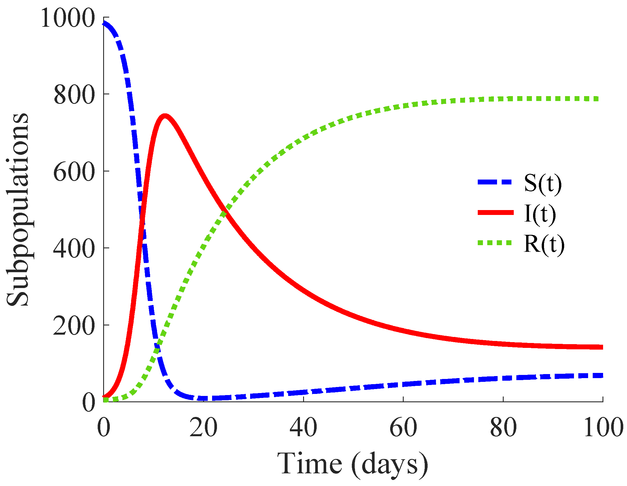
; that is, each primary infectious individual transmits the disease to more than 14 healthy individuals. Then, this example describes the propagation of a high infectivity disease. The DFE point of the model is unstable, while its EE point is globally asymptotically stable, as Remark 3 points out.
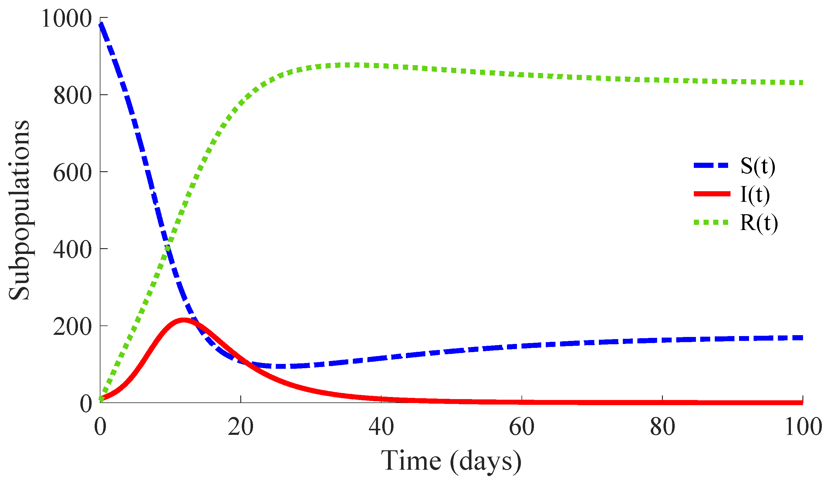
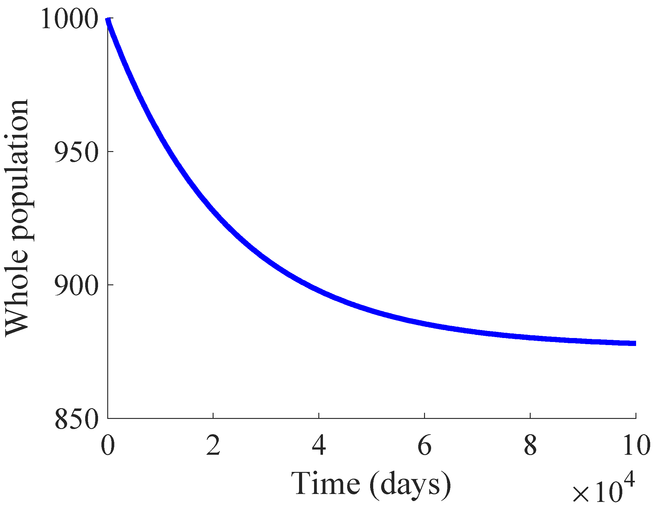
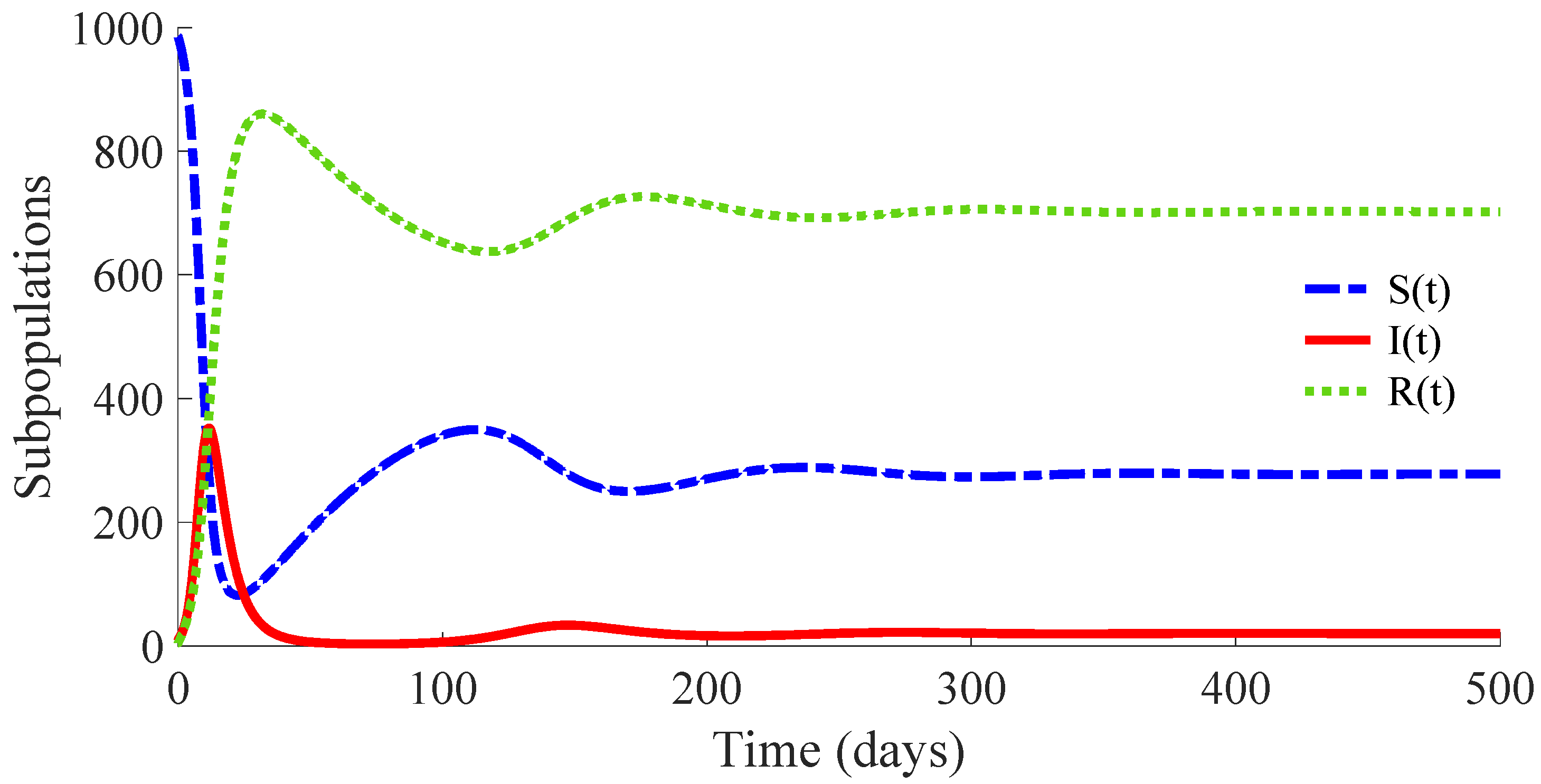
Figure 1 shows the time evolution of the susceptible, infectious, and recovered subpopulations during the first 100 days, while
Figure 2 displays that of the whole population in a very long time period. The considered initial condition is given by
,
and
.
In the longer simulation, one can see that the model tends to an EE point where the number of individuals is with , and accordingly to (14), (15) with , for . Although the mortality rate due to the disease is not very high, the influence of the disease is very important, since the whole population notably decreases from 1000 individuals to 877. Moreover, the percentage of infectious individuals with respect to the whole population in the EE point is 14.48%. In this situation, the application of control measures is crucial in order to eliminate the infection or, at least, to diminish its effect within the host population while reducing drastically the mortality.
3.2. Example 2: SIRS Model with Vaccination and Treatment
Models (1)–(3) with the same values for the parameters
,
,
,
,
and
as those given in Example 1 are considered. Moreover, a vaccination for newborn individuals together with the control actions (4) and (5) are applied in order to diminish the effects of the infectious disease. Concretely, the control actions are (i) a
vaccination of a proportion
of the
newborn individuals; i.e., 10% of newborns are vaccinated, (ii) a
vaccination of the susceptible population given by (4) with the values
,
,
and
for the associated parameters and (iii) a
treatment of the infectious population given by (5) with the values
and
for the corresponding parameters. Such values satisfy the conditions of Theorem 1 so that the model subpopulations and the vaccination and treatment efforts are non-negative for all time. The initial condition is that of Example 1 together with
for the initial control efforts. Note that dynamics of the treatment effort, given by the control law (5), is of first order with a gain that reaches the value
in the stationary regime. Such a gain points out a transition rate from the infectious subpopulation to the recovered one via applied treatment to be added to the transition rate
between such subpopulations from the natural response of the immunity system of the individuals against the disease. This fact points out that an infectious individual under treatment needs an average time of 5.54 days to overcome the disease. In this way, the average time of recovering is reduced in 16.46 days, since such an interval time is
days if no treatment is applied.
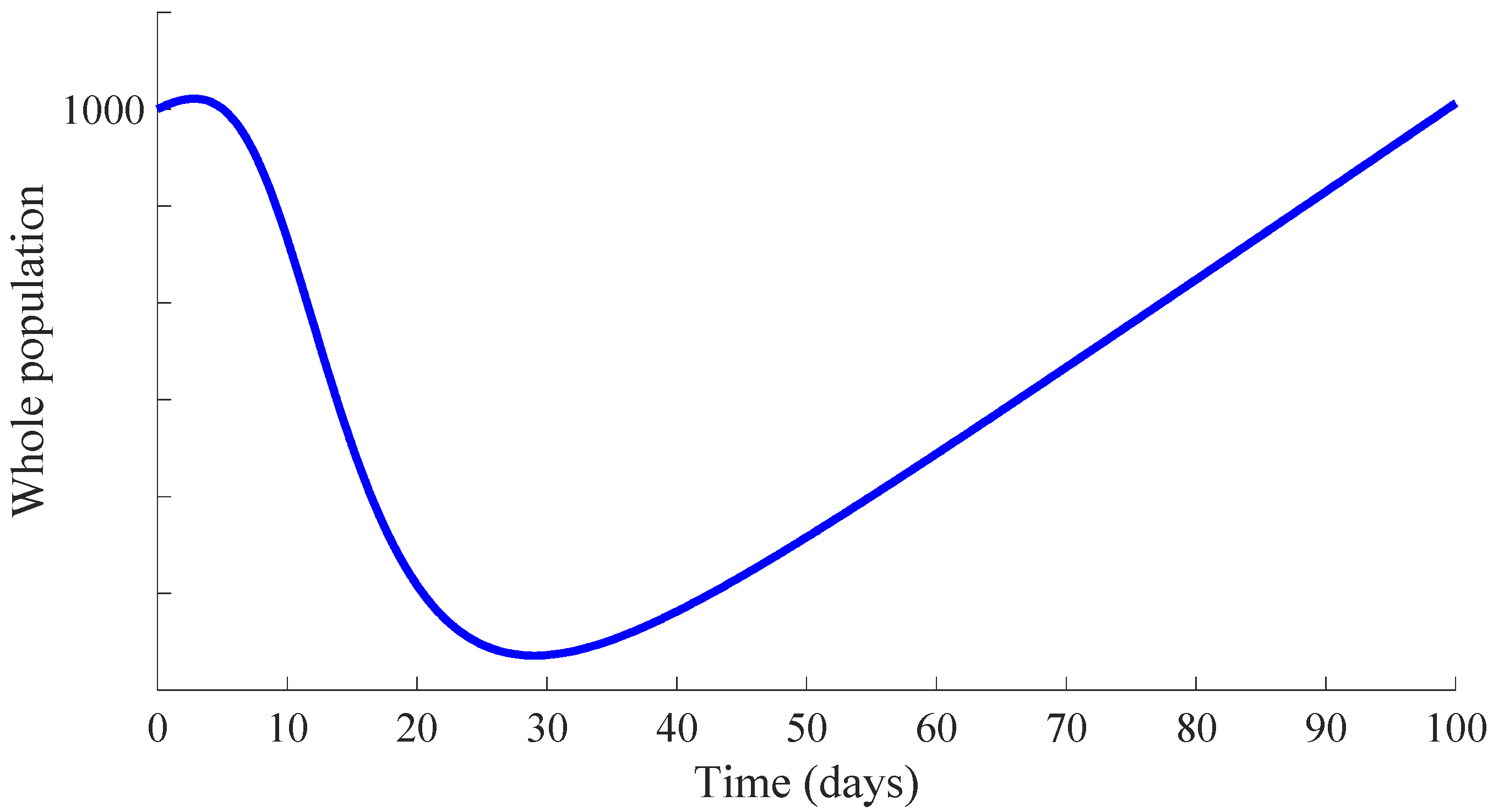
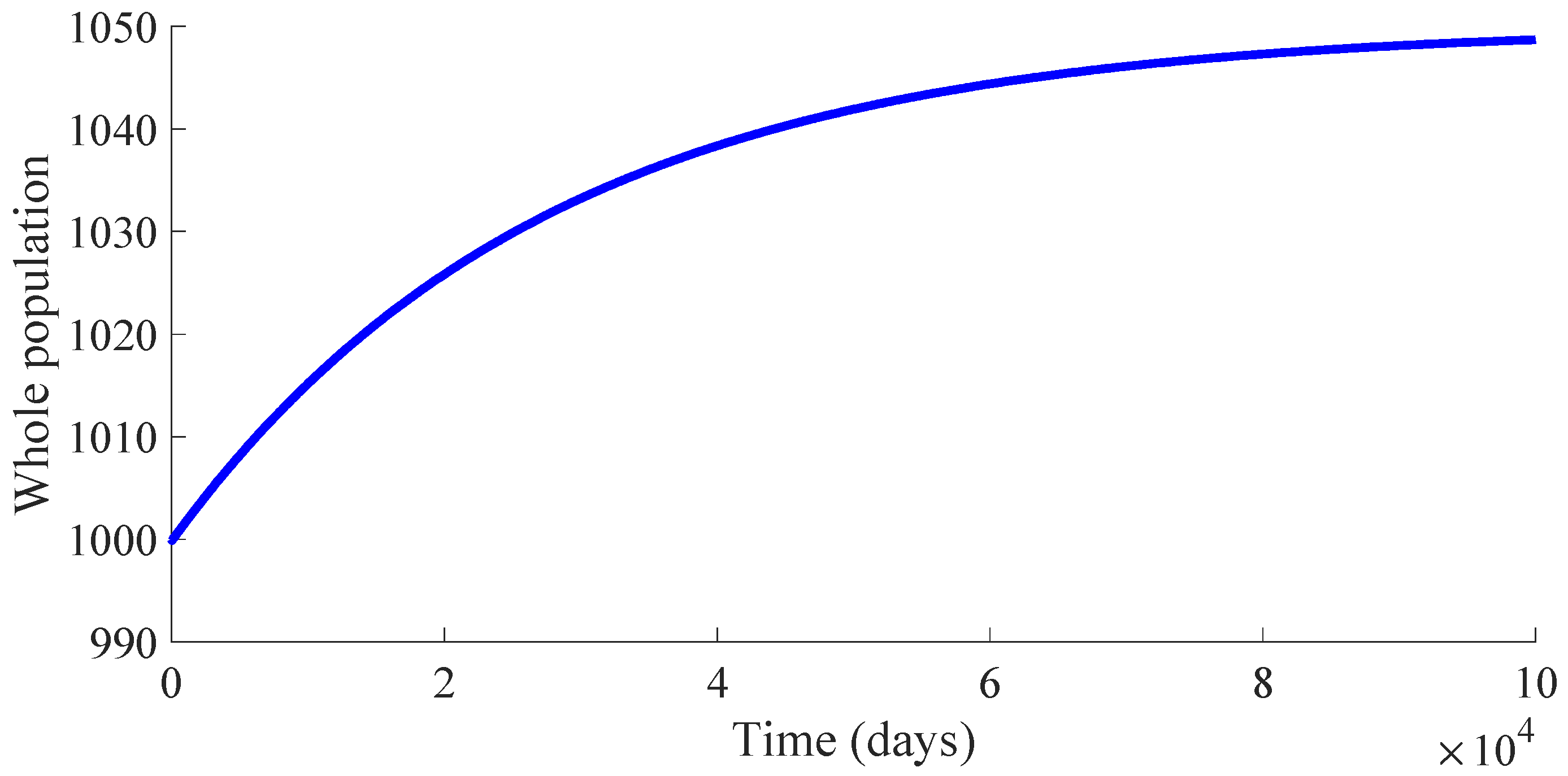
Figure 3 shows the time evolution of the susceptible, infectious, and recovered subpopulations during the first 100 days, while
Figure 4 and
Figure 5 display, respectively, that of the whole population during the first 100 days and along 100,000 days.
In a longer time performed simulation, one can see that the model tends to a DFE point where the number of individuals is
with
,
and
. This result is coherent with Theorems 3 and 4, since
,
and
for the used value
so that the DFE point is locally and globally asymptotically stable. Moreover, the choice of the control parameters satisfies the conditions of Theorem 2, which implies the non-existence of the EE point. Then, the DFE point is the unique equilibrium point for the controlled model. In summary, this example exhibits the high mortality reduction due to the application of the proposed feedback control actions in the propagation of an infectious disease of a high basic reproduction number
.
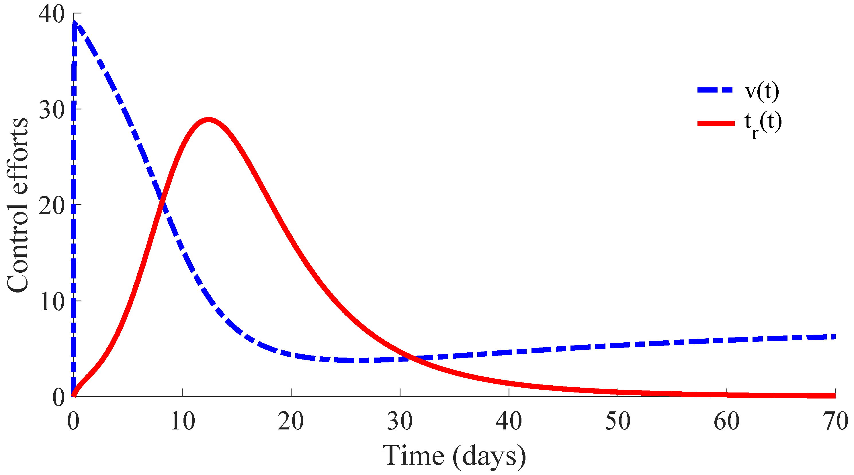
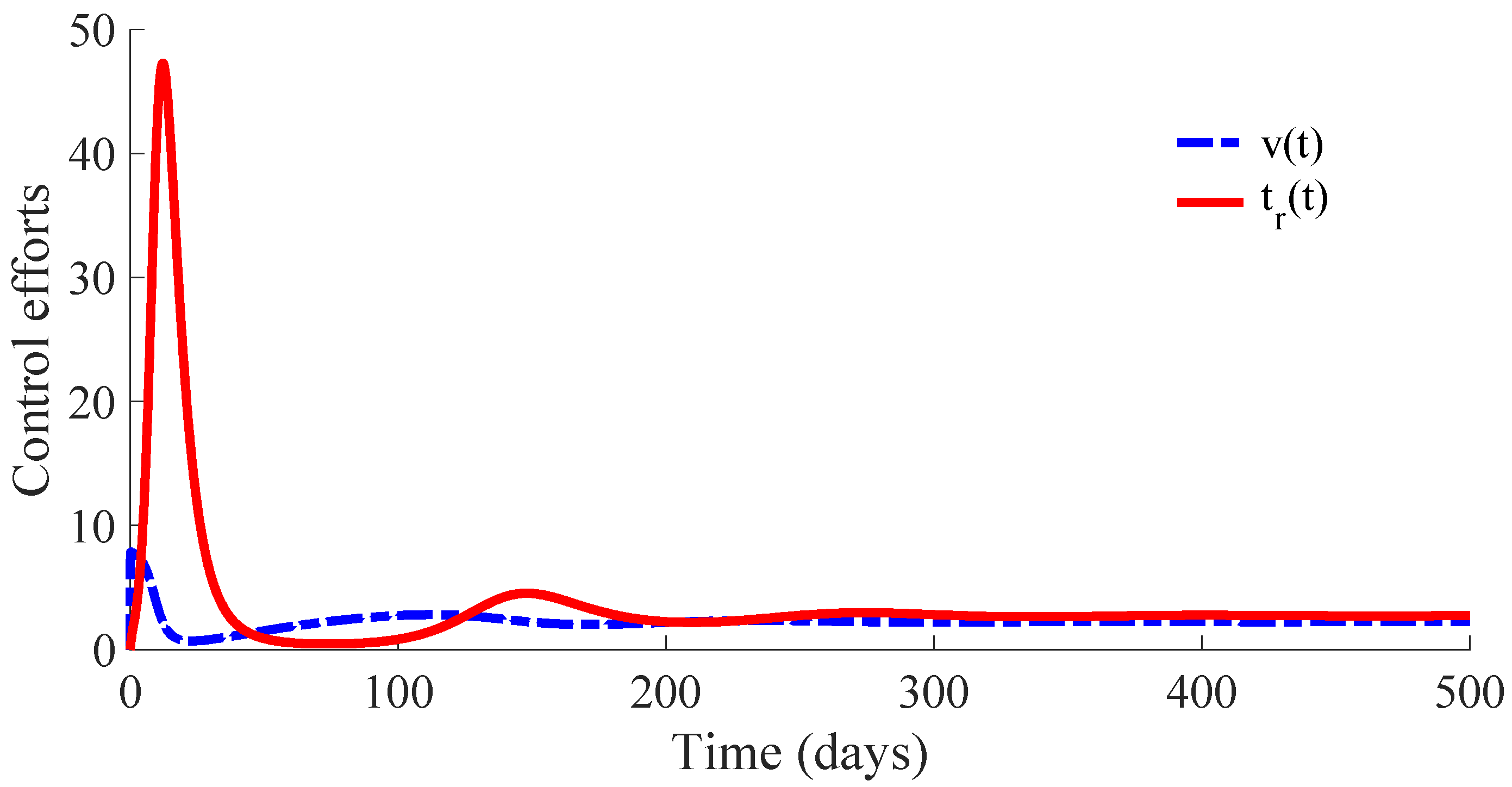
Figure 6 displays the time evolution of the control efforts. One can see that the treatment effort reaches a peak value when the number of infectious individuals reaches its maximum value, and then, such an effort converges to zero as a consequence of the convergence to zero of the infectious subpopulation. On the other hand, the vaccination effort converges to a constant value
.
The vaccination and treatment efforts can be interpreted as the number of vaccines and antivirals, or some appropriated medicaments, applied to the susceptible and infectious individuals, respectively, during the transition from the initial state to the DFE point. In this context, one can consider that the DFE point is reached when the number of infectious individuals is less than 1. Moreover, although the vaccination effort has a constant value
given by (10) at the DFE point, one can stop the vaccination control effort once the number of infectious individuals is smaller than 1. In this way, the vaccination can be set
once the DFE point is reached since the transition rate from the susceptible subpopulation to the infectious one is zero in the absence of infectious individuals due to such a rate depending on
. In other words, there is no propagation of the disease in absence of infectious individuals, and then, the vaccination can be stopped. However, the vaccination with the value
could be maintained as a preventive measure against possible new outbreaks of the disease due to immigration or other causes. This preventive measure gives place to a transition from the susceptible subpopulation to the recovered one with a rate that compensates for the transition rate
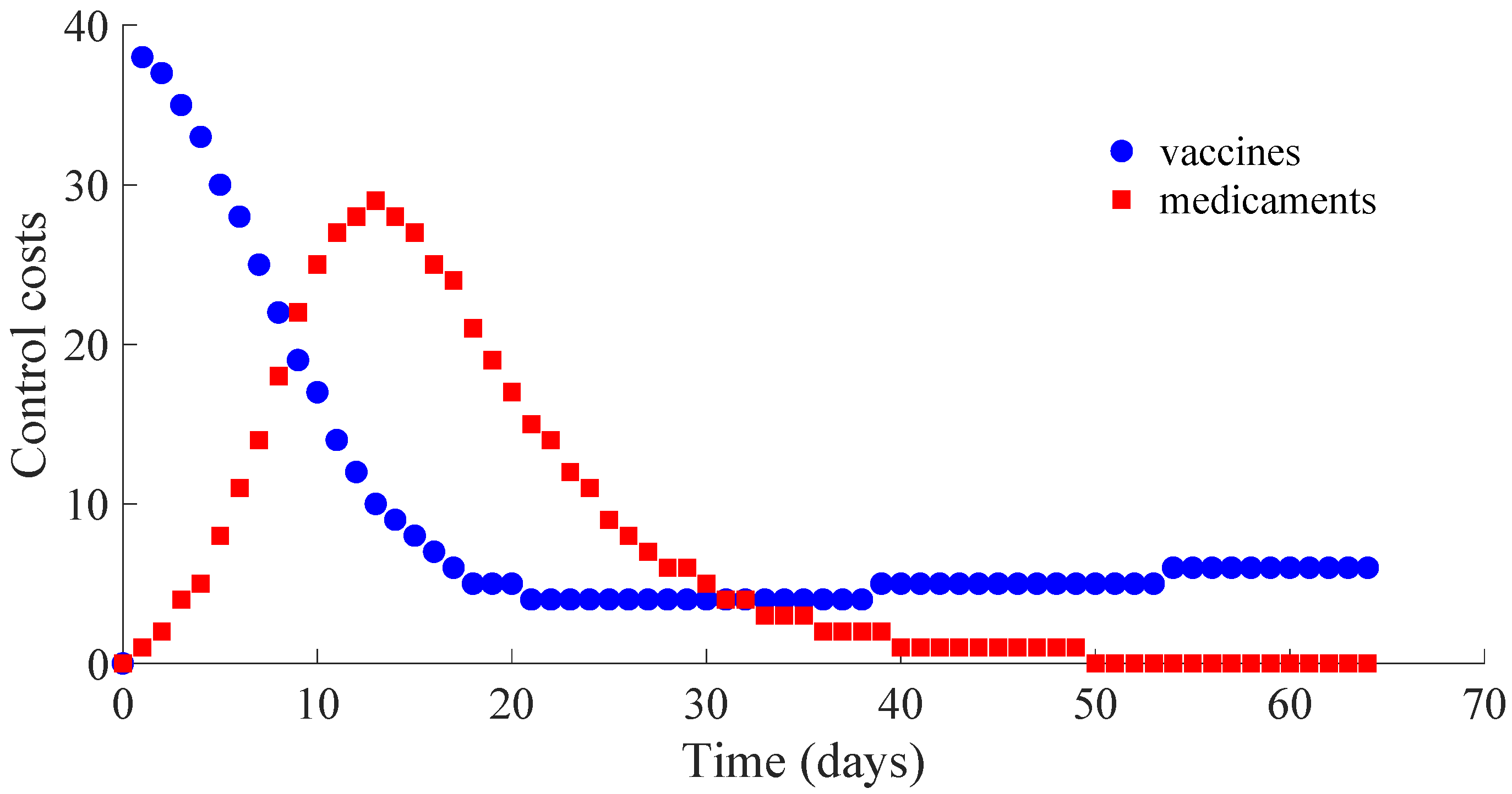
from the recovered subpopulation to the susceptible one caused by the immunity loss. In case that the vaccination is stopped once the DFE point is reached, which is at the 64th day in this example, the number of vaccines and medicaments applied to control the propagation in the transient from the initial day until achieving the DFE point are, respectively, 578 and 483. Such numbers can be interpreted as the control cost to eradicate the persistence of the disease.
Figure 7 displays the number of applied vaccines and medicaments each day during the transition to the DFE point. The numbers of vaccines and medicaments applied each day, respectively
and
, are obtained by evaluating
and
for all integer
with
denoting the day at which the DFE point is reached.
3.3. Example 3: SIRS Model with a Defective Vaccination and Treatment
The same values as those used in Example 2 for the parameters of the model are considered except that for
, which is replaced by
. In this way,
, while
. Then, the conditions of Theorem 2 are not satisfied, which implies that the non-existence of the EE point cannot be guaranteed. In fact, the time evolution of the subpopulations under these conditions is displayed in
Figure 8, and one can see that the EE point given by (14) and (15) is reached. Concretely, the whole number of individuals at the EE point is
with
,
, and
, and the vaccination and treatment control signals converge, respectively, to the values
and
.
The time evolution of the control efforts is displayed in
Figure 9.
3.4. Example 4: Study of the Influence of the Control Parameter on the Behaviour of the Controlled Model
Models (1)–(5) with the same values for the parameters as those given in Example 2, except that for
, are considered. In this way,
in all the analysed cases. Concretely, four cases are studied. Each one considers a different value for the parameter
in order to change slightly the ratio
, which implies a different value for the control reproduction number
. The condition
as well as the conditions of the Theorems 1, 2, 3, and 4 are satisfied in the four cases so that the DFE point is the unique equilibrium point, and it is locally and globally asymptotically stable, while the solutions of the controlled model are non-negative for all time under any non-negative initial condition. The interest of this study is to analyse the influence of the parameter
on the transition of the controlled model solutions from the initial state to the DFE point by evaluating the number of infectious individuals on each day as well as the cost of both vaccination and treatment control efforts. For such a purpose, the values for the control parameter
and then that of
in the four studied cases are: (i)
,
, (ii)
,
, (iii)
,
, and (iv)
,
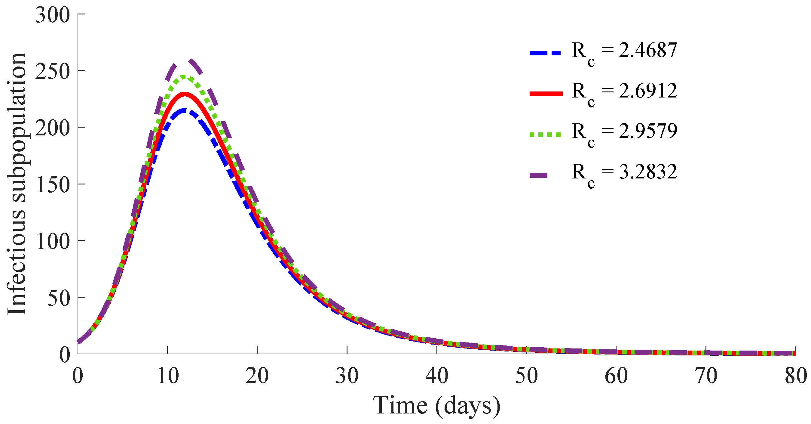
. Note that case (i) is that studied in Example 2, and it is used as the reference one for the current analysis. The initial condition is that used in Example 2 for all the cases.
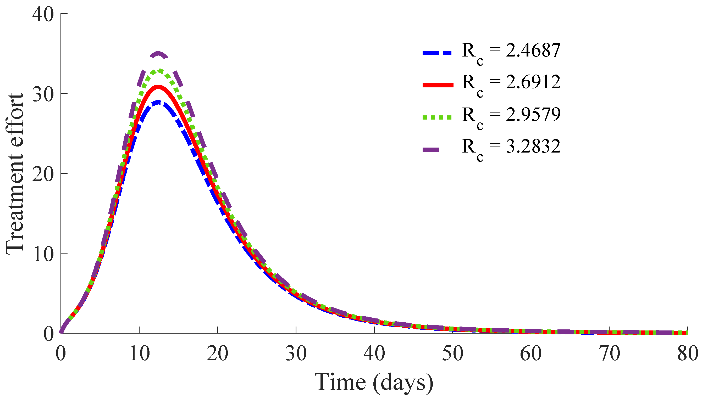
Figure 10 displays the time evolution of the infectious subpopulation in the four cases.
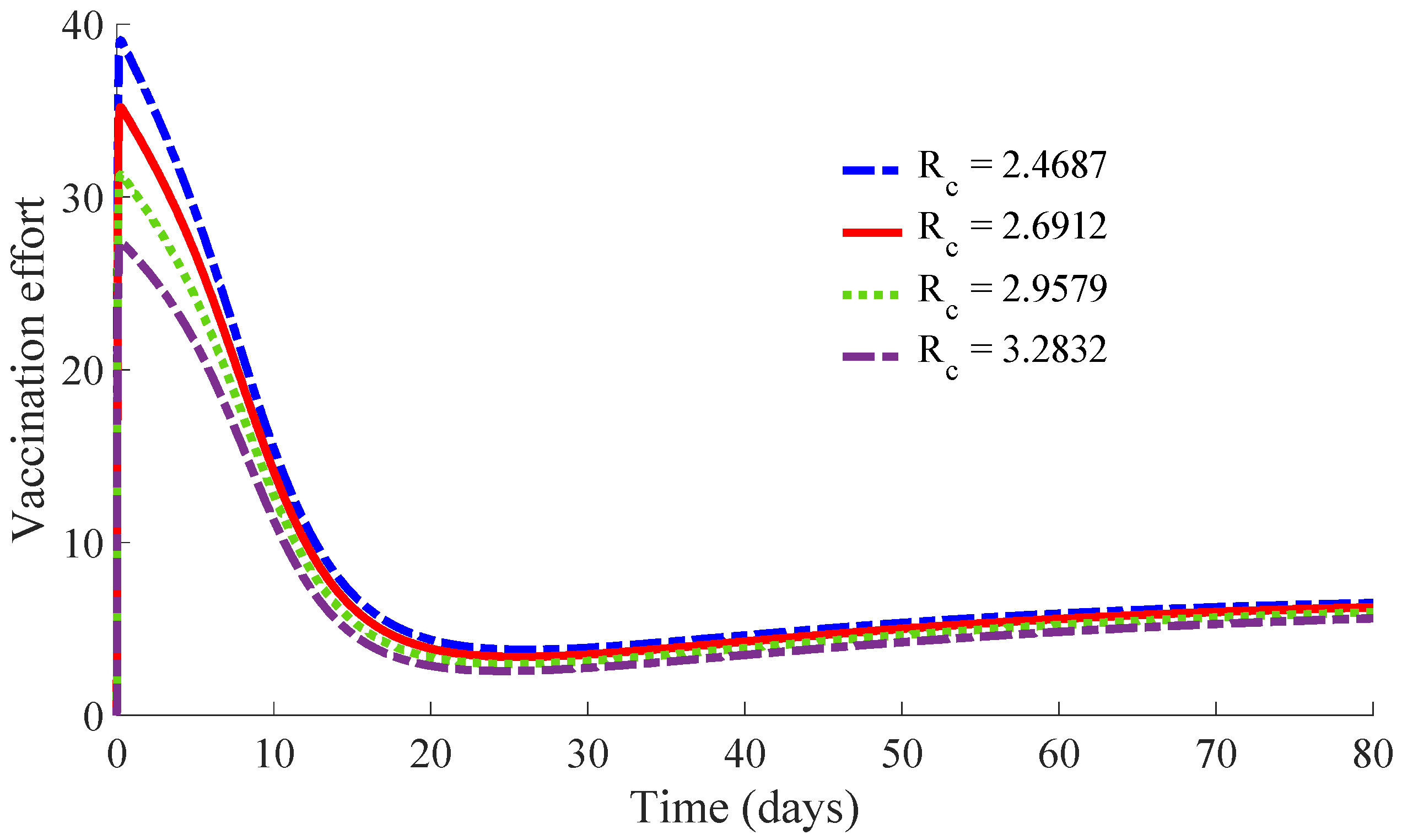
Figure 11 and
Figure 12 show, respectively, the time evolution of the vaccination and treatment efforts in the four cases.
One can see in these figures that the peaks in the infectious population, the vaccination and treatment efforts depend on the value of the control reproduction number
, which is established by the control parameters
and
. Concretely, the peak of the infectious subpopulation as well as that of the treatment effort increases as
increases, while the peak of the vaccination effort decreases as
increases, while maintaining
.
Table 1 summarises the most relevant specifications, included the aforementioned ones, about the four cases studied in this subsection.
The results show that the duration of the transient from the initial state to the DFE point increases as
increases. However, the number of vaccines applied during the whole transient period decreases when the value of
increases. Such a result is due to the fact that the peak of the vaccination effort decreases and, also, the number of vaccines used per day, when
increases. In summary, the number of required vaccines decreases while that of the required medicaments increases as
increases. Then, a tradeoff between the cost of vaccination and the number of infectious individuals with its associated treatment cost has to be taken into account for adjusting the values for the control parameters
and
. Such a tradeoff is going to depend on constraints about the number of available vaccines for the newborns and the susceptible individuals and/or medicaments for treatment of the infectious subpopulation. Finally,
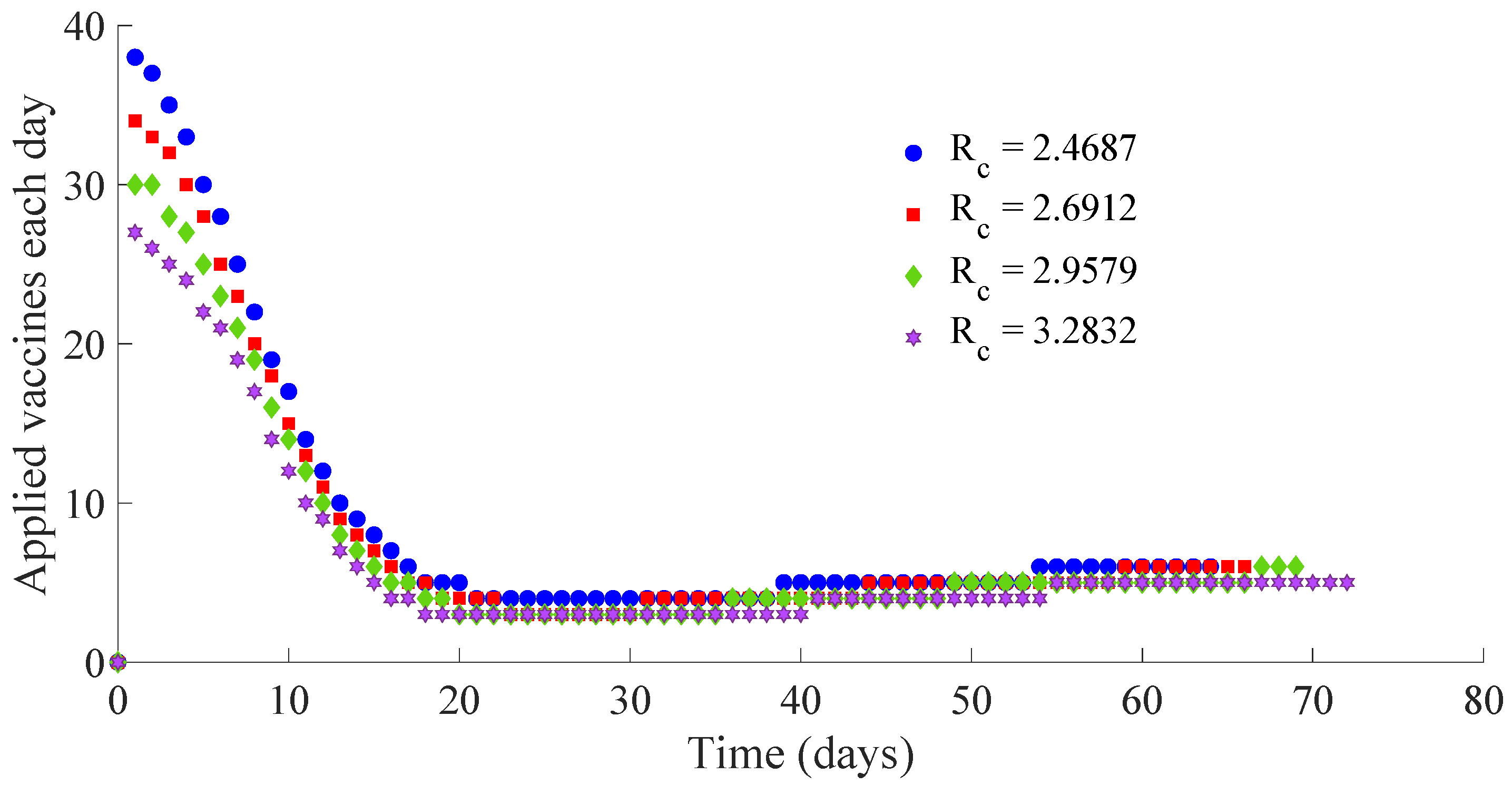
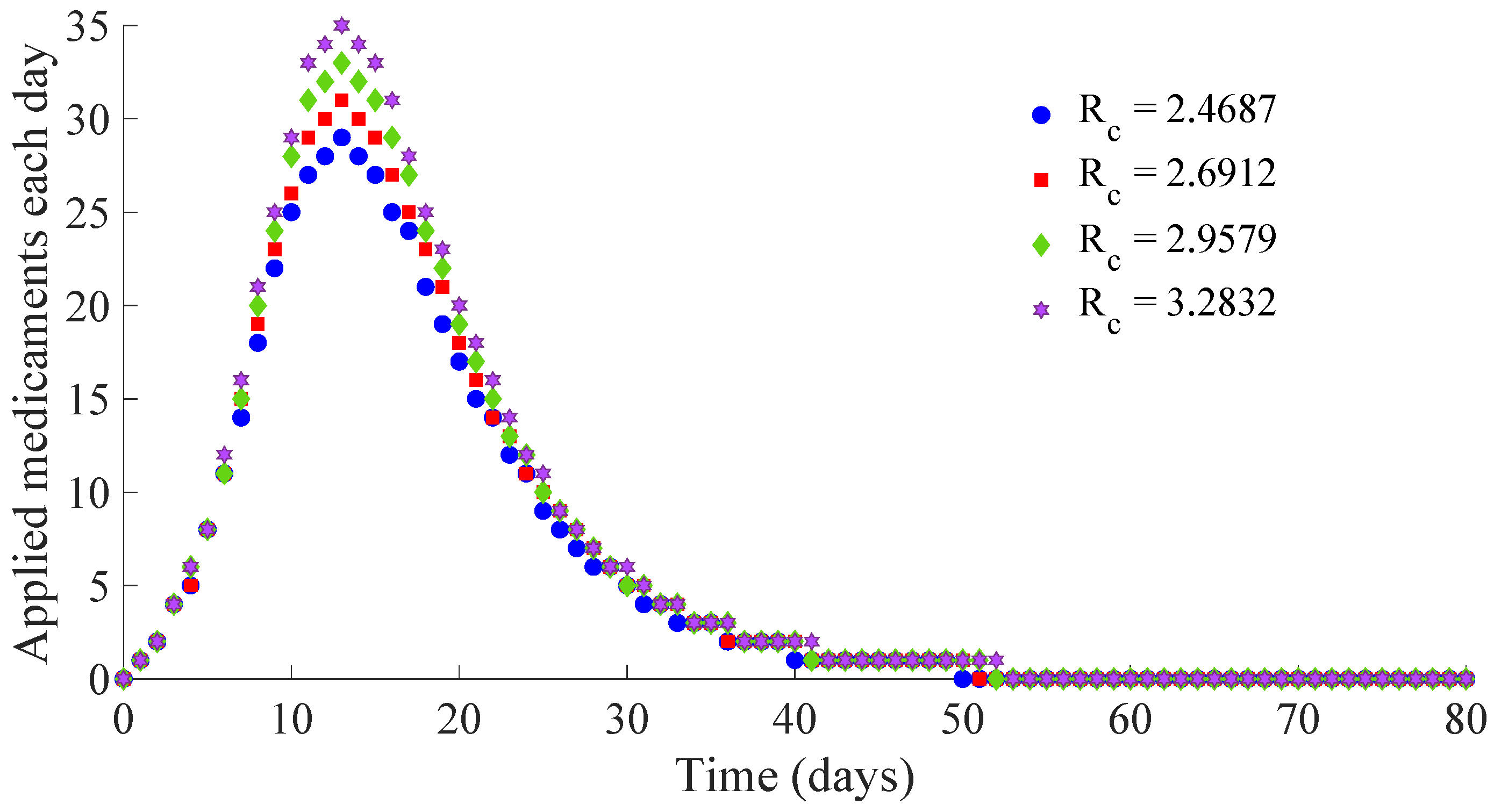
Figure 13 and
Figure 14 display the number of applied vaccines and medicaments each day during the transition to the DFE point for the four analysed cases.
One can see by analysing the results in
Table 1 and
Figure 10,
Figure 11,
Figure 12,
Figure 13 and
Figure 14 that the increase of the value of
, by decreasing the values of
, and maintaining the rest of the control parameters in the prescribed values, gives place to a decrease in the vaccination effort but both the infectious subpopulation and the applied treatment effort increase at the same time. The best of the studied cases from the viewpoint of the vaccination cost is case (iv), but it is not good enough from the viewpoint of both the treatment cost and the number of individuals who experience the infectious disease during the transition from the initial state until reaching the DFE point. In this context, it also seems interesting to examine the influence of the control parameter
, which take part in the dynamics of the treatment effort, on the specifications of the transient behaviour.
3.5. Example 5: Study of the Influence of the Control Parameter on the Behaviour of the Controlled Model
In the current example, the same values for the parameters
,
,
,
,
,
and
and for the initial condition as those given in Example 4 are considered. Furthermore, the values of
,
, and then
,
and
corresponding with the case of Example 4 with the smallest vaccination cost, concretely case (iv), which requires the application of 467 vaccines as one can see in
Table 1, are considered. Such a case is the worst scenario in Example 4 from the viewpoint of the time evolution of the infectious subpopulation and the cost in applied medicaments during the transient from the initial state to the DFE point; namely, 570 medicaments are required, as
Table 1 points out. The objective is to analyse the influence of the control parameter
, which acts on the value of
, on the specifications of such a transient time interval. Concretely, the value
is going to be considered in four proposed cases while the value for the parameter
will be modified in order to change slightly the ratio
. In this way, each case has a different transition rate from the infectious to recovered subpopulation due to the treatment action. Moreover, such a transition rate is added to the transition rate
from the infectious to the recovered subpopulation in the absence of treatment, i.e., that derived from the natural immunity system of the infectious individuals to fight against the disease. Such a fact implies a reduction in average for the recovering time of the infectious individuals. The analysed cases are (i)
,
, (ii)
,
, (iii)
,
, and (iv)
,
. Note that
as well as the conditions of the Theorems 1, 2, 3 and 4 are satisfied in all the cases so that the DFE point is the unique equilibrium point while being locally and globally asymptotically stable. Note also that case (ii) of this current example is the same as case (iv) of Example 4, which is used as the reference one for the current analysis. In case (i), the recovering time is reduced on average from
22 days, in absence of treatment, to
6.04 days if a treatment is applied following the rule (5). For cases (ii), (iii), and (iv), the recovering time passes from 22 to 5.54, 5.12, and 4.75 days, respectively. The values of
,
, and
are reached at the DFE point in the four analysed cases, as it can be deduced from (10), since all cases have the same values for
and
.
Figure 15 displays the time evolution of the infectious subpopulation, while
Table 2 summarises the specifications for these four studied cases.
One can see that the peak of the infectious subpopulation is decreasing as the value of and then also , increases. In addition, the number of required vaccines and medicaments during the transient decreases as the value for , and then also , increases. Such a result is mainly due to the fact that the duration of the transient decreases as the value of increases, since there is a small duration on average for the transition of individuals from infectious to the recovered subpopulation. Note also that the peak in the vaccination effort is equal for the four studied cases, since such a peak depends on the values of the parameters and , which are the same for the four cases. Case (iv) is the best of the analysed ones in the current study. It requires a strong treatment so that an infectious individual overcomes the infection after an average time of 4.75 days. In such a case, the transient from the initial state until arriving at the DFE point has the following characteristics:
The evolution of the infectious population reaches a peak of 215 individuals, i.e., approximately 21% of the initial whole population.
The vaccination cost during the transient supposes 428 vaccines, i.e., the percentage of the susceptible subpopulation to be vaccinated is around of the 43% of the initial population, assuming one vaccine per individual.
The treatment cost during the transient is of 554 medicaments, i.e., the percentage of infectious subpopulation to be treated is around 55% of the initial population, assuming one medicament per individual.
If the applied treatment has a lower performance so that the average recovering time is 5.54 days, corresponding to case (ii), instead of the 4.75 days of case (iv), then the peak of the infectious population is of 261 individuals, i.e., around the 26% of the initial population. In such a situation, the costs of vaccination and treatment are, respectively, 467 vaccines and 570 medicaments. In the considered worst case, i.e., case (i), which requires an average time of 6.04 days for the transition from the infectious to the recovered subpopulation, the number of necessary vaccines and medicaments is 525 and 573, respectively. As a conclusion, the transient duration and the cost in vaccines and medicaments are related with the performance of the applied treatment. If the applied medicaments have a poor potency such that the reduction of the recovery time is of a few days, then the duration of the transient from the initial state until reaching the DFE point can be very long. In such a case, the transient can be very expensive in relation with the number of required vaccines and medicaments or, even, the disease evolution can converge to the EE point if the resources in the number of medicaments and/or vaccines is not enough.
3.6. Example 6: Study of the Behaviour of the Controlled Model under Vaccination
The objective of this subsection is to study the dynamics of the controlled model when there are not medicaments for treating the infectious subpopulation, and then the only measure to control the propagation of the disease is the planning of a vaccination campaign to the newborns and the susceptible subpopulation. For this purpose, models (1)–(5) with
can be used with the initial condition
. In this way,
for all time. Moreover,
from (16) such that
is required to guarantee the non-existence of the EE point, and then, the DFE point is the unique equilibrium point while being locally and globally asymptotically stable. Since
, it is necessary that
to guarantee that
, and then, the eradication of the infectious disease can be achieved.
Table 3 compares the results obtained for seven different cases of values for the pair
and
, satisfying the conditions of the Theorems 1, 2, 3, and 4 so that the solutions of the controlled model are non-negative and the DFE point is the unique equilibrium point while being locally and globally asymptotically stable. The same values for the parameters
,
,
,
,
,
,
,
and
as those given in Example 2 are used, and the same initial condition is used as well.
The results in
Table 3 point out that the duration of the transient and also the peak in the infectious subpopulation decreases as the value for the parameter
decreases or, equivalently, as the ratio
increases. Such a decrease in the transient duration implies a smaller cost in the number of vaccines as
decreases. However, even in the cheapest case shown in
Table 3, i.e., case 7, the vaccination cost supposes the use of 1569 vaccines. Such a cost may be decreased even more by considering small values for
. In any case, the results show that the fight against the disease when there is not treatment and then, only the vaccination is available, is quite expensive. Moreover, the propagation of the disease can reach the EE point if there are not enough resources regarding vaccines. Note that the average rate for the transition from the susceptible subpopulation to the recovered one is approximately
or, equivalently, the average time in the transition of vaccinated individuals from the susceptible subpopulation to the recovered one is
days. In the cases studied in this subsection, such an average time is constrained between the values of 2.5 days, corresponding to case 1, and 1 day for case 7. Such a fact implies that the effect of the vaccination in the population is quite fast, less than 3 days, in any case. In this context, a more realistic scenario can be analysed by considering, for instance,
and
. In such a case,
, and the average time in the transition from the susceptible to the recovered subpopulation is 5 days. The specifications in the transient for this case are as follows:
Infectious peak: 92;
Transient duration: 235 days;
Number of vaccines: 2559;
, and .
One can see that the transient is very large, as it is the number of vaccines to be applied. In this context, the slower the effect of the vaccination in the population is, the larger the value of the parameter is as well as the duration of the transient and the number of vaccines to guarantee the eradication of the disease. Another alternative to deal with a more realistic scenario in the absence of treatment action could be the inclusion of a delay, corresponding to the reaction time of the vaccines, in the epidemic models (1)–(3).
3.7. Example 7: Study of the Behaviour of the Controlled Model under Treatment
The objective of this subsection is to study the dynamics of the controlled model when there are not vaccines for the newborns and the susceptible subpopulation, and then, the only measure to control the propagation of the disease is the application of some treatment to the infectious subpopulation. For this purpose, models (1)–(5) with
can be used with the initial condition
. In this way,
for all time. In this situation,
from (13), and such a value cannot be modified by control. However, a treatment procedure on the infectious population based on law (5) with appropriate values for the parameters
and
so that
can be designed. Since
, it is necessary that
to guarantee that
and then the non-existence of the EE point and the local and global asymptotic stability of the DFE point, which is the unique one in that case. In this way, the eradication of the infectious disease can be achieved. The current subsection compares the results obtained for some different cases satisfying the conditions of Theorems 1, 2, 3, and 4 so that the solutions of the controlled models are non-negative and the DFE point is the unique equilibrium point while being locally and globally asymptotically stable. Note that
is the rate of transition from the infectious subpopulation to the recovered one by means of treatment of infectious individuals and that such a transition rate is added to the average transition rate
between such subpopulations in the absence of treatment. By considering the same values for the parameters
,
,
and
as those used in Example 1, then
, and the transition rate
from treatment actions has to be strictly larger than
so that
, and then, the DFE point is the unique equilibrium point while being locally and globally asymptotically stable. This supposes an average time strictly smaller than
1.5387 days for recovering from the infectious disease. Such a situation is not realistic, since the existence of medicaments with such an extraordinary performance is improbable. By assuming that the non-existence of the EE point is not secured only with the applied treatment to the infectious subpopulation, at least, such a treatment campaign can reduce the effects of the disease in the whole population. Such a result is illustrated by considering several cases, concretely, those studied in Example 5 but without applying the vaccination of either the susceptible subpopulation, i.e.,
with
, or the newborns, i.e.,
. The results are presented in
Table 4 below.
One can see the decrease of the value of
due to the decrease of the value of
, which implies an increase of the average time that an infectious individual stays in the infectious subpopulation before passing to the recovered one, leads to a decrease in the number
of individuals in the whole population when the EE point is reached while increasing the percentage of infectious individuals at such an equilibrium point. In any case, the application of treatment reduces considerably the effects of the infectious disease if one compares the results of
Table 4 with those of Example 1 where no treatment is applied, and then, the whole population at the EE point is of 877 individuals with 127 infectious, i.e., 14.48% of individuals are infectious. Thus, the application of treatment reduces notably the high mortality and maintains the percentage of infectious subpopulation in reasonably small numbers at the achieved EE point.
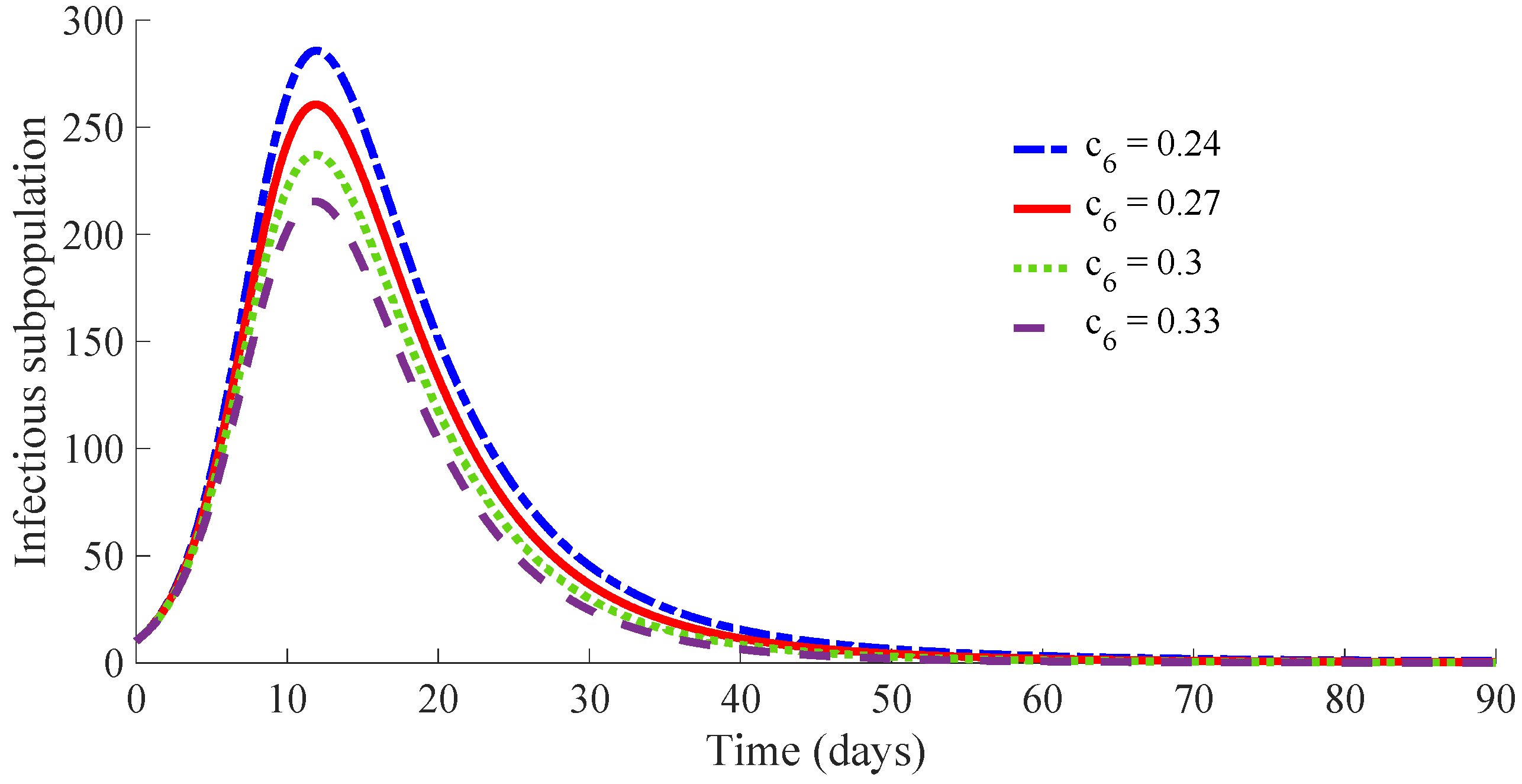
3.8. Example 8: Study of the Behaviour of the Controlled Model under Different Rates for the Loss of Immunity
The objective of this subsection is to study the dynamics of the controlled model under both control actions, vaccination and treatment, with different values of the rate
for the loss of immunity in the recovered subpopulation or, equivalently, different average periods of immunity for the recovered individuals. For this purpose, case (iv) of Example 4 can be taken as the reference one for this analysis, since it is one of the most convenient from the viewpoint of vaccination and treatment costs. The values of the model parameters are
,
,
,
,
and
, while those of the control actions are
,
,
,
,
,
and
in such a reference case. Other values for the parameter
are considered to analyse the influence of such a parameter on the transient specifications. Concretely, the following four cases are treated: (i)
,
(ii)
,
, (iii)
,
, and (iv)
,
. Note that case (ii) is used as a reference for this study and also note that the value of
has an influence on the value for
. In case (i), the average duration of the immunity is 100 days, and that of case (ii) is 120 days, while that of case (iii) is 150 days. Finally, there is no loss of immunity in case (iv). All the cases have the same values for
, namely
, so that
and then, the DFE point is locally and globally asymptotically stable for all the analysed cases. The results are presented in
Table 5 below.
One can see that the number of necessary vaccines and medicaments in the transient from the initial state to the DFE point decreases when the immunity period increases. Such a fact is mainly due to the transient period decreasing as the immunity period increases. Moreover, the number of recovery individuals at the DFE point increases when the immunity period increases.
4. Conclusions
An SIRS epidemic model with the vaccination of newborns and susceptible individuals and treatment of infectious ones has been investigated. The vaccination and the treatment are governed by a control subsystem containing several free-design parameters. This control subsystem provides two more free-design parameters comparing with those available in the more usual SIRS models with vaccination and treatment. In the proposed model, the intensity of both control actions is not directly proportional to the susceptible and/or infectious subpopulation, as it usually happens in the SIRS models. Here, both actions are provided by the control subsystem, and the parameters defining the dynamics of the controller are also available to shape the vaccination and treatment actions. This control strategy allows the achievement of several relevant results. First, an appropriate adjustment of the control parameters guarantees the positivity of the controller model, as it has been mathematically proved in Theorem 1. Note that such a property is required for coherence in epidemic models where all the subpopulations and the control actions, such as vaccination and treatment, have to be non-negative. Then, the equilibrium points of the proposed controlled epidemic model are calculated as a function of the system parameters. There are two equilibrium points: (i) the DFE point where the infectious subpopulation is zero and then the whole population is composed by susceptible and recovery subpopulations; and (ii) the EE point where the three subpopulations of the model are presented. The DFE one always exists while the existence of the EE point depends on the values of the control parameters. Moreover, the control reproduction number of the controlled epidemic model and a threshold value are mathematically obtained as functions of the control parameters. This result allows us to analyse the influence of the control parameters on both values and . In summary, the values and and the existence of the EE point depends on the control parameters. As a consequence, the existence of the EE point can be related with and . In this sense, values of the control parameters doing guarantee the non-existence of the EE point, as it has been mathematically proved in Theorem 2. In such a situation, the proposed controlled SIRS model only possesses a unique equilibrium point, namely, the DFE point. On the other hand, the local and global asymptotic stability of the DFE point are mathematically proved in Theorems 3 and 4, respectively. Then, an appropriate adjustment of the control parameters so that allows guaranteeing the positivity of the controlled epidemic model while ensuring the non-existence of the EE point. In such a situation, the DFE is the unique equilibrium point of the model, and then, the eradication of the infectious disease can be guaranteed.
Finally, the influence of the control parameters on the time evolution of the disease propagation has been studied by several simulation examples. The first example shows the time evolution of the propagation of the disease without applying control actions. One can see that the model converges to the EE point, and then, the disease is not eradicated. The second example shows the time evolution of the propagation of the disease if the proposed control actions are applied in an effective way, i.e., if the control parameters are chosen such that . In this case, one can see that the model converges to the DFE point, and the disease is eradicated. The third example shows the time evolution of the propagation of the disease if the proposed control actions are applied in a defective way, i.e., if the control parameters are chosen such that . One can see that the model converges to the EE point, and the disease is not eradicated. The fourth example analyses the influence of the controller parameter in the evolution of the propagation of the disease. Such a parameter acts in the vaccination control law, and it has an influence on the value of . Concretely, the value of is indirectly proportional to . This example shows that the model converges to the DFE point whenever . The number of vaccines and medicaments associated to the control efforts obtained from the control subsystem to achieve the DFE point depends on . One can see that by decreasing the value , or equivalently increasing the value of but guaranteeing that , the number of vaccines applied to the susceptible individuals decreases while that of medicaments applied to the infectious individuals increases. The fifth example analyses the influence of the controller parameter in the evolution of the propagation of the disease. Such a parameter acts in the treatment control law, and it has an influence on the value of . Concretely, the value of is directly proportional to . This example shows that the model converges to the DFE point whenever . The number of vaccines and medicaments associated to the control efforts obtained from the control subsystem to achieve the DFE point depends on . One can see that by increasing the value , or equivalently increasing the value of but guaranteeing that , the number of both vaccines and medicaments applied to the respective subpopulations decreases. Example 6 analyses the behaviour of the model when only the vaccination action is available. Example 7 analyses the behaviour of the model when only the treatment action is available. Example 6 shows that the DFE point is not achieved with an appropriate number of vaccines. Example 7 requires a treatment with a great potency so that the recovery of the infectious individuals after being treated is faster than in a real situation. Finally, Example 8 studies the evolution of the propagation for different rates of loss of immunity. The number of vaccines and medicaments in the convergence of the model to the DFE point decreases as the rate of losing immunity decreases.


