Inference for the Process Performance Index of Products on the Basis of Power-Normal Distribution

Abstract

The process performance index (PPI) can be a simple metric to connect the conforming rate of products. The properties of the PPI have been well studied for the normal distribution and other widely used lifetime distributions, such as the Weibull, Gamma, and Pareto distributions. Assume that the quality characteristic of product follows power-normal distribution. Statistical inference procedures for the PPI are established. The maximum likelihood estimation method for the model parameters and PPI is investigated and the exact Fisher information matrix is derived. We discuss the drawbacks of using the exact Fisher information matrix to obtain the confidence interval of the model parameters. The parametric bootstrap percentile and bootstrap bias-corrected percentile methods are proposed to obtain approximate confidence intervals for the model parameters and PPI. Monte Carlo simulations are conducted to evaluate the performance of the proposed methods. One example about the flow width of the resist in the hard-bake process is used for illustration.

1. Introduction

Control chart methods have been widely used as an online tool for process monitoring. After confirming the process is in control, practitioners can conduct a process capability analysis to determine how well the output of the process meets the expectations of customer, requirements, and specifications. The process capability analysis methods aim to continuously monitor the quality of process via using the capability indices for assuring that the products are consistent with the specifications, supplying information on product design and process quality improvement. Moreover, the results of process capability analysis can be the basis for reducing the cost due to product failures, see [1].

Among widely used process capability indices, the process performance index (PPI) can provide a close connection to the conforming rate of $P(X>L)$, where X is the quality variable and L is a given threshold about the lower quality limit. Ref. [2] recommended using the PPI to assess the quality of products under the normality assumption. The inferences of the PPI for the lifetime distributions with different censoring schemes also have been widely studied. Based on using a type-II censoring scheme, ref. [3] obtained the maximum likelihood estimate (MLE) of the PPI for the Pareto distribution. Moreover, they also proposed a hypothesis testing method to test PPI. Ref. [4] proposed an inference procedure to obtain the uniformly minimum variance unbiased estimate of PPI and conducted a hypothesis testing method for the two-parameter exponential distribution based on type-II censored samples. Ref. [5] proposed fourteen different estimates of the PPI for the two-parameter exponential distribution with a multiple type-II censoring scheme. Then, three estimates are screened from the pool to develop hypothesis testing procedures for testing PPI. Using a type-II censoring scheme, ref. [6] studied the statistical inference procedure for the PPI when the lifetimes follow an exponential distribution. Ref. [7] proposed some optimal statistical inferential procedures for the PPI based on progressively type-II censored samples for the Burr type XII distribution. Ref. [8] used generalized order statistics to conduct statistical inferences for the PPI when the lifetimes follow an exponential distribution. Ref. [9] proposed Bayesian estimation methods to assess the PPI when the progressive type-II censored samples are collected from Rayleigh distribution. Ref. [10] proposed parameter estimation methods to estimate the PPI based on progressive Weibull first-failure censored samples.

The power-normal family of distributions was first noted by [11]. They investigated the statistical properties of power-normal distribution and gave expressions for the moments in terms of infinite series. Ref. [12] studied the maximum likelihood estimation method to estimate the model parameters for the normalized power-normal distribution. Ref. [13] mentioned some applications about using the power-normal distribution. Ref. [14] presented another form of the power-normal distribution based on using inverse Box–Cox power transformation and obtained the expressions of the mean and variance of the power-normal distribution. Ref. [15] studied a truncated power-normal distribution that has the truncation point of zero. They studied the probabilistic properties along with the maximum likelihood and moments estimation methods. Ref. [16] used delta method to develop several estimation methods to obtain the confidence intervals of the percentiles of power-normal distribution. Ref. [17] investigated the closeness of power-normal distribution and skew-normal distribution and proposed estimation procedures to characterize skewed data via using the power-normal distribution. Ref. [18] evaluated the asymptotic influence of the truncation on the estimation of the parameters of the power-normal distribution via using an intensive simulation study.

The power-normal distribution is a generalized version of normal distribution. Moreover, the power-normal distribution can be a generalized family and more competitive than skew-normal distribution to characterize real data if the skewness parameter in the skew-normal distribution is small. In this study, we aim to propose a reliable estimation process to evaluate the PPI in quality control applications. The proposed estimation process can be used to evaluate the PPI whatever the data follow a symmetric or asymmetric distribution. Moreover, the new estimation process can involve the estimation method based on normality assumption as special case.

We investigate the maximum likelihood estimation method and the confidence interval method based on using the exact Fisher information matrix. Moreover, we also study the weakness of using an exact Fisher information matrix to obtain the confidence intervals of the power-normal distribution parameters. Two bootstrap methods are used to obtain the approximate confidence interval of PPI when the quality characteristic follows a power-normal distribution.

2. Motivation and Organization

The probability density function (PDF) and cumulative density function (CDF) of the power-normal are defined, respectively, by

$$\begin{array}{c}\hfill f\left(y\right|\mathsf{\Theta })=\frac{\gamma }{\sigma }{\left[\mathsf{\Phi }\left(\frac{y-\xi }{\sigma }\right)\right]}^{\gamma -1}\varphi \left(\frac{y-\xi }{\sigma }\right), y\in R,\xi \in R,\gamma >0,\sigma >0,\end{array}$$

(1)

and

$$\begin{array}{c}\hfill F\left(y\right|\mathsf{\Theta })={\left[\mathsf{\Phi }\left(\frac{y-\xi }{\sigma }\right)\right]}^{\gamma }, y\in R,\xi \in R,\gamma >0,\sigma >0,\end{array}$$

(2)

where $\mathsf{\Theta }=(\xi ,\gamma ,\sigma )$, and $\xi$ is the location parameter, $\sigma$ is the scale parameter and $\gamma$ is the shape parameter. When $\gamma =1$, the power-normal distribution reduces to the normal distribution with the mean $\xi$ and standard deviation $\sigma$. The power-normal distribution is left-skewed if $0<\gamma <1$ and right-skewed if $\gamma >1$. The power-normal distribution can be an alternative to the skew-normal distribution proposed by Azzalini [19].

Process capability analysis methods often are used to evaluate whether the quality of products meets customers’ requirements. Define the PPI by

$$C_L=\frac{\xi -L}{\sigma }.$$

(3)

If the quality variable X follows a normal distribution, $\xi$ and $\sigma$ are respectively the mean and standard deviation of X. Throughout this article, a product is labeled as satisfactory if the condition of $\{X>L\}$ is satisfied. The probability of a satisfactory product is known as the conforming rate and defined by

$${\eta }_L=P\left\{X\ge L\right\}.$$

(4)

There is a connection between the conforming rate ${\eta }_L$ and $C_L$ when X follows a parametric distribution. This fact implies that the statistical inference for the conforming rate may be used as well for the $C_L$ and vice versa.

In the real world, the distribution of quality variables could not have a symmetric shape. Hence, the existing inference methods based on the normality assumption for $C_L$ become not available. It is important to develop new inference methods to assess the quality of $C_L$ for a wide range of distribution shapes and the new method can also be applied to the normal distribution. The skew-normal distribution proposed by Azzalini [19] can be an option to characterize process data. However, the skew-normal distribution is not the best model in terms of capturing high degrees of kurtosis. The quality of the estimation results based on the skew-normal distribution is not stable if the skewness parameter is close to zero. In order to overcome the weakness of the skew-normal distribution for the inferences about $C_L$. We suggest replacing the skew-normal distribution with the power-normal distribution to develop new inference methods for $C_L$.

The power-normal distribution is available to characterize the data whose distribution has a higher degree of kurtosis than the normal and skew-normal distributions but has a narrow range of asymmetry. Based on the aforementioned reasons, we aim to develop a maximum likelihood estimation procedure for the power-normal distribution and investigate the weakness of using an exact Fisher information matrix to obtain the confidence intervals of the model parameters and $C_L$. Moreover, two parametric bootstrapping procedures are developed in this study to obtain approximate confidence intervals of the power-normal distribution parameters and $C_L$.

The Fisher information matrix and bootstrap methods are two extensively used methods to obtain approximate confidence intervals of the model parameters. If the exact Fisher information matrix can be obtained, the delta method and exact Fisher information matrix can be used to obtain an approximate confidence interval of a function of model parameters. If the exact Fisher information matrix is not available, the observed Fisher information matrix can be used instead. Because the obtained approximate confidence interval via using the delta method and Fisher information matrix is based on the Central Limit Theorem, the obtained approximate confidence interval could be conservative with an over-or under-estimated coverage probability.

The bootstrap is a computer-based method which can replace the delta method to obtain an approximate confidence interval of a function of model parameters. The bootstrap often is used to derive an estimate of standard error or confidence interval of a complex estimator of the interest parameter. In quality control or reliability applications, bootstrap has been extensively used to obtain the approximate confidence interval of a complex estimator of the interest parameter. Among all bootstrap methods, the parametric bootstrap percentile (PBP) and bias-corrected percentile (BCP) methods are two popular methods to obtain the approximate confidence interval of a complex estimator of the interest parameter. Comprehensive processes to construct bootstrap confidence intervals can be found in [20]. Quality control and reliability applications based on using bootstrap methods can be found in [21,22,23,24].

The rest of this paper is organized as follows: In Section 3, the maximum likelihood estimation procedure is proposed and the exact Fisher information matrix is derived. Moreover, the steps to implement the PBP and BCP methods are developed. We also study the drawbacks of using the exact Fisher information matrix to obtain an approximate confidence interval for the model parameters and PPI. In order to evaluate the performance of the proposed estimation methods, an intensive Monte Carlo simulation study is conducted in Section 4 to evaluate the performance of the proposed maximum likelihood estimation method in terms of the metrics of bias and mean squared error (MSE). The performance of the interval inference methods is evaluated based on the coverage probability (CR) for the target parameter. In Section 5, the applications of the proposed estimation procedures are illustrated with one real example about the flow width of the resist in a hard-bake process. Finally, some concluding remarks are given in Section 6.

3. The Inference Methods

3.1. Maximum Likelihood Estimation Method

Based on the power-normal distribution defined by Equations (1) and (2), the maximum likelihood estimation procedure is proposed in this section. Let $X=\frac{Y-\xi }{\sigma }$, the $m$th moment of Y can be obtained by

$$\begin{array}{c}\hfill E\left[Y^m\right]=\sum _{l=0}^m\left(\genfrac{}{}{0pt}{}{m}{l}\right){\xi }^l{\sigma }^{m-l}E\left[X^{m-l}\right],\end{array}$$

(5)

where X has the PDF

$$f\left(x\right|\gamma )=\gamma {\left[\mathsf{\Phi }\left(x\right)\right]}^{\gamma -1}\varphi \left(x\right), x\in R.$$

The PDF of $y_i$ can be presented by

$$f\left(y_i\right|\mathsf{\Theta })=\frac{\gamma }{\sigma }{\left(\mathsf{\Phi }\left(\frac{y_i-\xi }{\sigma }\right)\right)}^{\gamma -1}\varphi \left(\frac{y_i-\xi }{\sigma }\right)=\frac{\gamma }{\sigma }{\left(\mathsf{\Phi }\left(x_i\right)\right)}^{\gamma -1}\varphi \left(x_i\right), i=1,2,\cdots ,n.$$

Let $\mathit{y}=y(y_1,y_2,\dots ,y_n)$ denote a random sample of $y^{\prime }s$. The likelihood function and log-likelihood function of $\mathit{y}$ can be presented by

$$\begin{array}{c}\hfill L\left(\mathsf{\Theta }\right|\mathit{y})=\prod _{i=1}^{n}f\left(y_i\right|\mathsf{\Theta })=\frac{{\gamma }^n}{{\sigma }^n}\prod _{i=1}^n{\left(\mathsf{\Phi }\left(x_i\right)\right)}^{\gamma -1}\prod _{i=1}^n\varphi \left(x_i\right),\end{array}$$

(6)

where $x_i=\frac{y_i-\xi }{\sigma }$ and

$$\begin{array}{ccc}\hfill \ell & =& \log \left(L\right(\mathsf{\Theta }\left|\mathit{y}\right))\hfill \\ & =& n(\log \left(\gamma \right)-\log \left(\sigma \right))+(\gamma -1)\sum _{i=i}^n\log \left(\mathsf{\Phi }\left(x_i\right)\right)\hfill \\ & & +\sum _{i=i}^n\log \left(\varphi \left(x_i\right)\right).\hfill \end{array}$$

(7)

The first and second derivatives of ℓ with respect to $\xi ,\sigma$ and $\gamma$ can be obtained by

$$\begin{array}{c}\hfill \frac{\partial \ell }{\partial \xi }=\frac{1}{\sigma }\left[\sum _{i=1}^n{x}_i-(\gamma -1)\sum _{i=1}^n\frac{\varphi \left(x_i\right)}{\mathsf{\Phi }\left(x_i\right)}\right],\end{array}$$

(8)

$$\begin{array}{c}\hfill \frac{\partial \ell }{\partial \gamma }=\frac{n}{\gamma }+\sum _{i=1}^n\log \left(\mathsf{\Phi }\left(x_i\right)\right),\end{array}$$

(9)

$$\begin{array}{c}\hfill \frac{\partial \ell }{\partial \sigma }=\frac{1}{\sigma }\left[\sum _{i=1}^n{x}_i^2-n-(\gamma -1)\sum _{i=1}^n\frac{x_i\varphi \left(x_i\right)}{\mathsf{\Phi }\left(x_i\right)}\right],\end{array}$$

(10)

$$\begin{array}{c}\hfill \frac{{\partial }^2\ell }{\partial {\xi }^2}=-\frac{1}{{\sigma }^2}\left\{n+(\gamma -1)\sum _{i=1}^n\left[\frac{x_i\varphi \left(x_i\right)}{\mathsf{\Phi }\left(x_i\right)}+\frac{{\varphi }^2\left(x_i\right)}{{\mathsf{\Phi }}^2\left(x_i\right)}\right]\right\},\end{array}$$

(11)

$$\begin{array}{c}\hfill \frac{\partial {\ell }^2}{\partial {\gamma }^2}=-\frac{n}{{\gamma }^2},\end{array}$$

(12)

$$\begin{array}{ccc}\hfill \frac{{\partial }^2\ell }{\partial {\sigma }^2}& =& -\frac{1}{{\sigma }^2}\left\{3\sum _{i=1}^n{x}_i^2-n-(\gamma -1)\left\{\sum _{i=1}^n\frac{(2x_i-x_i^3)\varphi \left(x_i\right)}{\mathsf{\Phi }\left(x_i\right)}\right.\right.\hfill \\ & & \left.\left.-\sum _{i=1}^n\frac{x_i^2{\varphi }^2\left(x_i\right)}{{\mathsf{\Phi }}^2\left(x_i\right)}\right\}\right\},\hfill \end{array}$$

(13)

$$\begin{array}{c}\hfill \frac{{\partial }^2\ell }{\partial \xi \partial \gamma }=-\frac{1}{\sigma }\sum _{i=1}^n\frac{\varphi \left(x_i\right)}{\mathsf{\Phi }\left(x_i\right)},\end{array}$$

(14)

$$\begin{array}{ccc}\hfill \frac{{\partial }^2\ell }{\partial \xi \partial \sigma }& =& -\frac{1}{{\sigma }^2}\left\{2\sum _{i=1}^n{x}_i+(\gamma -1)\left[\sum _{i=1}^n\frac{(x_i^2-1)\varphi \left(x_i\right)}{\mathsf{\Phi }\left(x_i\right)}\right.\right.\hfill \\ & & \left.\left.+\sum _{i=1}^n\frac{x_i{\varphi }^2\left(x_i\right)}{{\mathsf{\Phi }}^2\left(x_i\right)}\right]\right\},\hfill \end{array}$$

(15)

and

$$\begin{array}{c}\hfill \frac{\partial {\ell }^2}{\partial \gamma \partial \sigma }=-\frac{1}{\sigma }\sum _{i=1}^n\frac{x_i\varphi \left(x_i\right)}{\mathsf{\Phi }\left(x_i\right)}.\end{array}$$

(16)

Let $\frac{\partial \ell }{\partial \xi }=0$, $\frac{\partial \ell }{\partial \sigma }=0$, and $\frac{\partial \ell }{\partial \gamma }=0$, we can obtain the following three likelihood equations:

$$\begin{array}{c}\hfill \sum _{i=1}^n{x}_i=(\gamma -1)\sum _{i=1}^n\frac{\varphi \left(x_i\right)}{\mathsf{\Phi }\left(x_i\right)},\end{array}$$

(17)

$$\begin{array}{c}\hfill \sum _{i=1}^n{x}_i^2=n+(\gamma -1)\sum _{i=1}^n\frac{x_i\varphi \left(x_i\right)}{\mathsf{\Phi }\left(x_i\right)},\end{array}$$

(18)

$$\begin{array}{c}\hfill \gamma =-\frac{n}{{\sum }_{i=1}^n\log \left(\mathsf{\Phi }\left(x_i\right)\right)}.\end{array}$$

(19)

Let $\kappa \left(\mathsf{\Theta }\right)$ be a differentiable function of $\mathsf{\Theta }$. Denote the gradient of $\kappa \left(\mathsf{\Theta }\right)$ by $\nabla \kappa \left(\mathsf{\Theta }\right)=\left(\frac{\partial \kappa \left(\mathsf{\Theta }\right)}{\partial \xi },\frac{\partial \kappa \left(\mathsf{\Theta }\right)}{\partial \sigma },\frac{\partial \kappa \left(\mathsf{\Theta }\right)}{\partial \gamma }\right)$. The MLE of $\kappa \left(\mathsf{\Theta }\right)$ can be denoted by $\kappa \left(\widehat{\mathsf{\Theta }}\right)$ though using the invariance property of MLE. For simplicity, let $\widehat{\kappa }\equiv \kappa \left(\widehat{\mathsf{\Theta }}\right)$ and let $\nabla \kappa \left(\widehat{\mathsf{\Theta }}\right)$ be the plug-in version of $\nabla \kappa \left(\mathsf{\Theta }\right)$. An approximate confidence interval of $\kappa \left(\mathsf{\Theta }\right)$ can be obtained using Theorem 1.

Theorem 1. 

Let $\mathit{I}\left(\mathsf{\Theta }\right)$ denote the exact Fisher information matrix. Based on Equations (8)–(16) and delta method, the asymptotic distribution of $\widehat{\kappa }$ can be obtained by

(a) 

$$\widehat{\kappa }\to N\left(\mathsf{\Theta },(\nabla \kappa \left(\widehat{\mathsf{\Theta }}\right)){\left(\mathit{I}\left(\widehat{\mathsf{\Theta }}\right)\right)}^{-1}{(\nabla \kappa \left(\widehat{\mathsf{\Theta }}\right))}^T\right) \mathrm{as} n\to \infty .$$

(b) 

The approximate confidence interval of $C_L$ can be presented by

$${\widehat{C}}_L\to N\left(C_L,\left(\frac{1}{\widehat{\sigma }},0,-\frac{\widehat{\xi }-L}{{\widehat{\sigma }}^2}\right){\left(\mathit{I}\left(\widehat{\mathsf{\Theta }}\right)\right)}^{-1}{\left(\frac{1}{\widehat{\sigma }},0,-\frac{\widehat{\xi }-L}{{\widehat{\sigma }}^2}\right)}^T\right) \mathrm{as} n\to \infty ,$$

where $C_L$ is the PPI of the power-normal distribution and defined by

$$C_L=\frac{\xi -L}{\sigma }.$$

The approximate $(1-\alpha )\%$ confidence interval of $C_L$ can be obtained by

$$\begin{array}{c}\hfill {\widehat{C}}_L\pm z_{\alpha /2}\times \sqrt{\left(\frac{1}{\widehat{\sigma }},0,-\frac{\widehat{\xi }-L}{{\widehat{\sigma }}^2}\right){\left(\mathit{I}\left(\widehat{\mathsf{\Theta }}\right)\right)}^{-1}{\left(\frac{1}{\widehat{\sigma }},0,-\frac{\widehat{\xi }-L}{{\widehat{\sigma }}^2}\right)}^T}.\end{array}$$

(20)

Proof. 

(a)

The MLEs of $\xi$, $\sigma$ and $\gamma$ can be the simultaneous solutions of the Equations (17)–(19). Denote them by $\widehat{\xi }$, $\widehat{\sigma }$ and $\widehat{\gamma }$, respectively, and let $\widehat{\mathsf{\Theta }}=(\widehat{\xi },\widehat{\gamma },\widehat{\sigma })$. Let ${\delta }_{11}=-E\left(\frac{{\partial }^2\ell }{\partial {\xi }^2}\right)$, ${\delta }_{22}=-E\left(\frac{{\partial }^2\ell }{\partial {\gamma }^2}\right)$, ${\delta }_{33}=-E\left(\frac{{\partial }^2\ell }{\partial {\sigma }^2}\right)$, ${\delta }_{12}={\delta }_{21}=-E\left(\frac{{\partial }^2\ell }{\partial \xi \partial \gamma }\right)$, ${\delta }_{13}={\delta }_{31}=-E\left(\frac{{\partial }^2\ell }{\partial \xi \partial \sigma }\right)$, ${\delta }_{23}={\delta }_{32}=-E\left(\frac{{\partial }^2\ell }{\partial \gamma \partial \sigma }\right)$, We obtain the following results:

$$\begin{array}{c}\hfill {\delta }_{11}=\frac{n}{{\sigma }^2}\left\{1+(\gamma -1)\left[E\left(X\frac{\varphi \left(X\right)}{\mathsf{\Phi }\left(X\right)}\right)+E\left(\frac{{\varphi }^2\left(X\right)}{{\mathsf{\Phi }}^2\left(X\right)}\right)\right]\right\},\end{array}$$

(21)

$$\begin{array}{c}\hfill {\delta }_{22}=\frac{n}{{\gamma }^2},\end{array}$$

(22)

$$\begin{array}{ccc}\hfill {\delta }_{33}& =& \frac{n}{{\sigma }^2}\left\{3E\left(X^2\right)-1-(\gamma -1)\left[E\left((2X-X^3)\frac{\varphi \left(X\right)}{\mathsf{\Phi }\left(X\right)}\right)\right.\right.\hfill \\ & & \left.\left.-E\left(X^2\frac{{\varphi }^2\left(X\right)}{{\mathsf{\Phi }}^2\left(X\right)}\right)\right]\right\},\hfill \end{array}$$

(23)

$$\begin{array}{c}\hfill {\delta }_{12}=\frac{n}{\sigma }E\left(\frac{\varphi \left(X\right)}{\mathsf{\Phi }\left(X\right)}\right),\end{array}$$

(24)

$$\begin{array}{c}\hfill {\delta }_{13}=\frac{n}{{\sigma }^2}\left\{2E\left(X\right)+(\gamma -1)\left[E\left(\left(X^2-1\right)\frac{\varphi \left(X\right)}{\mathsf{\Phi }\left(X\right)}\right)+E\left(X\frac{{\varphi }^2\left(X\right)}{{\mathsf{\Phi }}^2\left(X\right)}\right)\right]\right\},\end{array}$$

(25)

and

$$\begin{array}{c}\hfill {\delta }_{23}=\frac{n}{\sigma }E\left(X\frac{\varphi \left(X\right)}{\mathsf{\Phi }\left(X\right)}\right).\end{array}$$

(26)

Hence, the exact Fisher information matrix can be presented by

$$\mathit{I}\left(\mathsf{\Theta }\right)=\left[\begin{array}{ccc}{\delta }_{11}& {\delta }_{12}& {\delta }_{13}\\ {\delta }_{21}& {\delta }_{22}& {\delta }_{23}\\ {\delta }_{31}& {\delta }_{32}& {\delta }_{33}\end{array}\right].$$

Because $\mathit{I}\left(\mathsf{\Theta }\right)$ contains unknown parameters, the plug-in version of $\mathit{I}\left(\mathsf{\Theta }\right)$, denoted by $\mathit{I}\left(\widehat{\mathsf{\Theta }}\right)$, can be used to find the asymptotic distribution of $\widehat{\mathsf{\Theta }}$. We can be shown that

$$\widehat{\mathsf{\Theta }}\to N\left(\mathsf{\Theta },{\left(\mathit{I}\left(\widehat{\mathsf{\Theta }}\right)\right)}^{-1}\right) \mathrm{as} n\to \infty .$$

The delta method indicates that the asymptotic mean and variance of $\widehat{\kappa }$ are $\kappa \left(\mathsf{\Theta }\right)$ and $\nabla \kappa \left(\widehat{\mathsf{\Theta }}\right){\left(\mathit{I}\left(\widehat{\mathsf{\Theta }}\right)\right)}^{-1}{(\nabla \kappa \left(\widehat{\mathsf{\Theta }}\right))}^T$, respectively. Moreover, using Central limit theorem, we can show that the asymptotic distribution of $\widehat{\kappa }$ is normal. Hence, we can show that

$$\widehat{\kappa }\to N\left(\kappa \left(\mathsf{\Theta }\right),(\nabla \kappa \left(\widehat{\mathsf{\Theta }}\right)){\left(\mathit{I}\left(\widehat{\mathsf{\Theta }}\right)\right)}^{-1}{(\nabla \kappa \left(\widehat{\mathsf{\Theta }}\right))}^T\right) \mathrm{as} n\to \infty .$$

We prove Theorem 1a.

(b)

Using invariant property, the MLE of $C_L$ can be obtained by

$$\begin{array}{c}\hfill {\widehat{C}}_L=\frac{\widehat{\xi }-L}{\widehat{\sigma }}.\end{array}$$

(27)

The gradient of $C_L$ is $\nabla C_L=\left(\frac{\partial C_L}{\partial \xi },\frac{\partial C_L}{\partial \gamma },\frac{\partial C_L}{\partial \sigma }\right)=\left(\frac{1}{\sigma },0,-\frac{\xi -L}{{\sigma }^2}\right)$. Moreover, we can show that the asymptotical variance of ${\widehat{C}}_L$ is

$$\left(\frac{1}{\widehat{\sigma }},0,-\frac{\widehat{\xi }-L}{{\widehat{\sigma }}^2}\right){\left(\mathit{I}\left(\widehat{\mathsf{\Theta }}\right)\right)}^{-1}{\left(\frac{1}{\widehat{\sigma }},0,-\frac{\widehat{\xi }-L}{{\widehat{\sigma }}^2}\right)}^T$$

and the asymptotic distribution of ${\widehat{C}}_L$ can be obtained by

$${\widehat{C}}_L\to N\left(C_L,\left(\frac{1}{\widehat{\sigma }},0,-\frac{\widehat{\xi }-L}{{\widehat{\sigma }}^2}\right){\left(\mathit{I}\left(\widehat{\mathsf{\Theta }}\right)\right)}^{-1}{\left(\frac{1}{\widehat{\sigma }},0,-\frac{\widehat{\xi }-L}{{\widehat{\sigma }}^2}\right)}^T\right) \mathrm{as} n\to \infty .$$

Then, the approximate $(1-\alpha )\%$ confidence interval of $C_L$ can be obtained by

$$\begin{array}{c}\hfill {\widehat{C}}_L\pm z_{\alpha /2}\times \sqrt{\left(\frac{1}{\widehat{\sigma }},0,-\frac{\widehat{\xi }-L}{{\widehat{\sigma }}^2}\right){\left(\mathit{I}\left(\widehat{\mathsf{\Theta }}\right)\right)}^{-1}{\left(\frac{1}{\widehat{\sigma }},0,-\frac{\widehat{\xi }-L}{{\widehat{\sigma }}^2}\right)}^T}.\end{array}$$

(28)

We prove Theorem 1b. □

If $\gamma =1$, $C_L$ reduces to the PPI of the normal distribution. Hence, the $C_L$ is a generalized PPI which can be used as a performance metric under skew distributions and including the normal distribution as special case.

3.2. Bootstrap Methods

Parametric bootstrap methods are other widely used methods to obtain an approximate $(1-\alpha )\times 100\%$ confidence interval of $\kappa \left(\mathsf{\Theta }\right)$. In this study, the parametric bootstrap methods of PBP and BCP are developed to obtain the approximate $(1-\alpha )\times 100\%$ confidence interval of $\kappa \left(\mathsf{\Theta }\right)$. Readers can see [20] for comprehensive introductions to the PBP and BCP methods. The procedures to implement the PBP and BCP methods are presented as follows:

• The PBP method

The $(1-\alpha )\%$ bootstrap confidence interval of $\kappa \left(\mathsf{\Theta }\right)$ based on the PBP method can be obtained based on the following steps:

Step 1:

Obtain the MLE of $\mathsf{\Theta }$ based on a large sample of size n and denote the MLE by $\widehat{\mathsf{\Theta }}$.

Step 2:

Generate a bootstrap sample of size n from the power-normal distribution with parameter $\mathsf{\Theta }=\widehat{\mathsf{\Theta }}$.

Step 3:

Implement Step 2 B times, where B is a large number and denote all obtained MLE of $\mathsf{\Theta }$ by ${\widehat{\mathsf{\Theta }}}_j^{*}$, $j=1,2,\cdots ,B$. Let ${\widehat{\kappa }}_j^{*}\equiv \widehat{\kappa }\left({\widehat{\mathsf{\Theta }}}_j^{*}\right)$, $j=1,2,\cdots ,B$ be the MLE of $\kappa \left(\mathsf{\Theta }\right)$ based on B bootstrap samples.

Step 4:

Construct the empirical distribution of $\widehat{\kappa }$ based on the bootstrap samples $\left\{{\widehat{\kappa }}_j^{*}, j=1,2,\cdots ,B\right\}$ and denote the empirical distribution of $\widehat{\kappa }$ by ${\widehat{G}}_{\kappa }^{*}$. The $(1-\alpha )\%$ bootstrap confidence interval of $\kappa \left(\mathsf{\Theta }\right)$ can be obtained by $(g_{\alpha /2},g_{1-\alpha /2})$, where $g_p$ is the $p$th quantile function of ${\widehat{G}}_{\kappa }^{*}$ such that ${\widehat{G}}_{\kappa }^{*}\left(g_p\right)=p$ for $0<p<1$.

• The BCP method

The $(1-\alpha )\%$ bootstrap confidence interval of $\kappa \left(\mathsf{\Theta }\right)$ based on the BCP method can be obtained based on the following steps:

Step 1:

Implement Step 1 to Step 3 of the PBP method to obtain the bootstrap sample of ${\widehat{\kappa }}_j^{*}\equiv \widehat{\kappa }\left({\widehat{\mathsf{\Theta }}}_j^{*}\right),j=1,2,\dots ,B$.

Step 2:

The approximate $(1-\alpha )$ confidence interval of $\kappa \left(\mathsf{\Theta }\right)$ can be obtained by

$$\left({\left({\widehat{G}}_{\kappa }^{*}\right)}^{-1}\mathsf{\Phi }[z_{\alpha /2}+2{\mathsf{\Phi }}^{-1}\left({\widehat{G}}_{\kappa }^{*}\left(\widehat{\kappa }\right)\right)],{\left({\widehat{G}}_{\kappa }^{*}\right)}^{-1}\mathsf{\Phi }[z_{1-\alpha /2}+2{\mathsf{\Phi }}^{-1}\left({\widehat{G}}_{\kappa }^{*}\left(\widehat{\kappa }\right)\right)]\right).$$

3.3. Discussions

From Theorem 1, we find that the approximate confidence interval of $C_L$ in Theorem 1b is available only if the exact Fisher information matrix, $\mathit{I}\left(\mathsf{\Theta }\right)$, in Theorem 1a exists. The existence of $\mathit{I}\left(\mathsf{\Theta }\right)$ depends on the MLE of $\gamma$. For example, the component of $E\left(X\frac{{\varphi }^2\left(X\right)}{{\varphi }^2\left(X\right)}\right)$ in ${\delta }_{13}$ exists only if $\gamma \ge 3$. Because $\gamma$ is an unknown parameter in practical applications, this limitation makes the use of $\mathit{I}\left(\mathsf{\Theta }\right)$ difficult. Considering the sampling error for estimating model parameters, we could obtain an MLE of $\gamma$ smaller than 3 if the value of $\gamma$ is larger but close to 3. If $\gamma <3$, $\mathit{I}\left(\mathsf{\Theta }\right)$ cannot be obtained. The existence of $\mathit{I}\left(\mathsf{\Theta }\right)$ causes a difficulty to use the approximate confidence interval that is obtained via using Theorem 1. Based on the aforementioned reasons, we suggest using the two proposed parametric bootstrap methods to obtain an approximate confidence interval for the model parameters and $C_L$ in practical applications.

The power-normal distribution can be a generalized version of normal distribution. In literature, some extended versions of the power-normal distribution have been proposed. For example, the log-power-normal distribution and truncated-power-normal distribution. Hence, these extended versions have a more complicated function form than the power-normal distribution and contain more parameters to characterize data. The extended versions of the power-normal distribution have a merit with a complicated shape to model data. However, the parameter estimation could be a problem. If a distribution contains two or more shape (or skewness) parameters, the model identification could be a problem for practical use. Two distributions with different combinations of plug-in estimates can fit the same data set well.

In our experience, two different distributions could result in different tail percentiles. Percentiles are important for quality control or reliability applications. Hence, the complexity of the model form and obtaining reliable parameter estimation results are trade-off. To avoid an over-fitting problem, we suggest using a generalized version of normal distribution to model data and such generalized version can include the normal distribution as special case. Based on the purpose, the skew-normal distribution and power-normal distribution are competitive. The power-normal distribution is available to characterize the data whose distribution has a higher degree of kurtosis than the normal and skew-normal distributions but has a narrow range of asymmetry. Moreover, the estimation results are less reliable based on the skew-normal distribution if its skewness parameter is small. That is, if the distribution of data is slightly asymmetric, the estimation results based on skew-normal distribution could be less reliable if the sample size is not large enough. In this study, we recommend using power-normal distribution and the developed inference processes to characterize data.

4. Monte Carlo Simulations

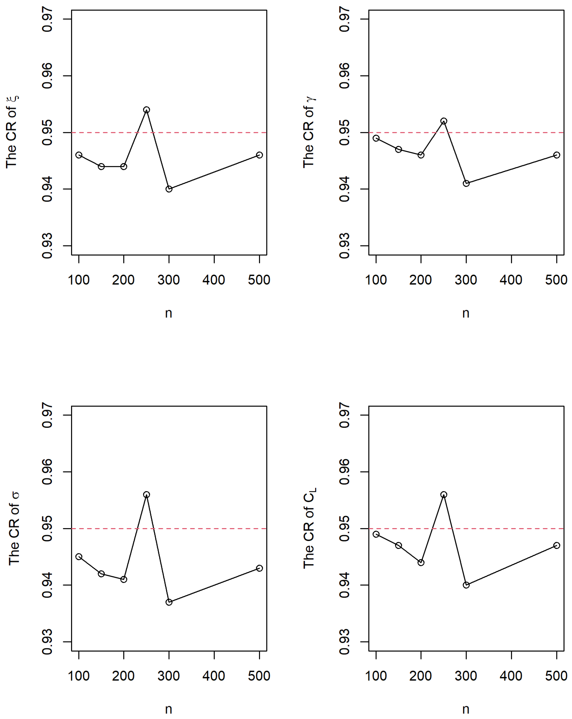
In this section, Monte Carlo simulations are conducted to evaluate the performance of the proposed maximum likelihood estimation method and the two parametric bootstrap methods. Because the power-normal distribution reduces to normal distribution when $\gamma =1$, the first goal of the design of the Monte Carlo simulation is to study the estimation performance of the MLE of $\gamma$ and its impacts on the estimation performance of the MLEs of the location and scale parameters in the power-normal distribution. Based on the aforementioned purposes, the Monte Carlo simulations are conducted with the parameters of $\xi =3$, $\sigma =1$ and $\gamma =0.5,1,2$ and 5. The estimation performance is evaluated in terms of the scale-free metrics based on the bias and MSE. Define the bias and MSE of a parameter of $\theta$ by $\mathrm{Bias}=\frac{1}{M}{\sum }_{i=1}^M({\widehat{\theta }}_i-\theta )$ and $\mathrm{MSE}=\frac{1}{M}{\sum }_{i=1}^M{({\widehat{\theta }}_i-\theta )}^2$, respectively, where ${\widehat{\theta }}_i$ is the MLE of $\theta$ for the $i^{\mathrm{th}}$ iteration, $i=1,2,\cdots ,M$ and M is a big positive integer. The relative bias and the relative square root of the MSE of $\widehat{\theta }$ can be defined respectively by

$$\mathrm{rBias}=\frac{1}{\theta }\times \mathrm{Bias}$$

and

$$\mathrm{rsqMSE}=\frac{1}{\theta }\times \sqrt{\mathrm{MSE}}.$$

In this study, $\theta$ can be $\xi$, $\gamma$, $\sigma$ and $C_L$. We use M = 10,000 iterations to evaluate the values of rBias and rsqMSE. Moreover, we also evaluate the number of any absolute MLEs of $\xi$, $\gamma$ and $\sigma$ larger than ten times of their true parameters in 10,000 simulation runs, and denote this obtained number by $N_u$. All simulation results are reported in

Table 1. The rBias and rsqMSEs of the MLEs of $\xi$, $\gamma$, $\sigma$ and $C_L$.

		rBias				rsqMSE
$\mathit{\gamma }$	$\mathit{n}$	$\widehat{\mathit{\xi }}$	$\widehat{\mathit{\gamma }}$	$\widehat{\mathit{\sigma }}$	${\widehat{\mathit{C}}}_{\mathit{L}}$	$\widehat{\mathit{\xi }}$	$\widehat{\mathit{\gamma }}$	$\widehat{\mathit{\sigma }}$	${\widehat{\mathit{C}}}_{\mathit{L}}$	${\mathit{N}}_{\mathit{u}}$
0.5	100	0.2096	−0.5994	−1.2269	1.1320	0.7258	33.0214	2.0278	2.2301	240
	150	0.2390	−2.6064	−1.2264	0.8151	0.6571	13.5733	2.0054	1.4548	70
	200	0.2434	−2.9725	−1.2176	0.6825	0.6370	4.8467	1.9865	1.1086	25
	250	0.2475	−3.1008	−1.2152	0.6299	0.6251	4.5750	1.9792	0.9567	11
	300	0.2462	−3.1453	−1.2109	0.5905	0.6134	4.5548	1.9772	0.8447	8
	500	0.2544	−3.2785	−1.2104	0.5447	0.5987	4.5559	1.9692	0.7335	0
1	100	0.2712	3.0260	−0.9345	0.8341	0.6417	26.4524	1.4044	2.2745	511
	150	0.3016	0.4983	−0.9383	0.5427	0.5659	14.5790	1.3798	1.3561	212
	200	0.3241	−0.2356	−0.9473	0.4684	0.5425	4.6232	1.3725	0.9842	94
	250	0.3276	−0.4745	−0.9443	0.4186	0.5235	3.5571	1.3619	0.8349	33
	300	0.3337	−0.6071	−0.9467	0.3985	0.5155	1.8356	1.3588	0.7632	26
	500	0.3420	−0.7792	−0.9463	0.3538	0.4969	1.4421	1.3504	0.6235	2
2	100	0.2551	7.9755	−0.8761	0.2849	0.6422	45.1581	1.2072	2.4265	1126
	150	0.2928	2.6819	−0.8825	0.0267	0.5485	16.8547	1.1900	1.4013	652
	200	0.3273	1.2177	−0.9007	−0.0075	0.5182	7.0036	1.1902	1.0722	402
	250	0.3281	0.8255	−0.8962	−0.0736	0.4936	4.0130	1.1793	0.8994	261
	300	0.3342	0.5714	−0.8965	−0.0970	0.4778	2.4949	1.1746	0.8284	159
	500	0.3510	0.2852	−0.9045	−0.1194	0.4655	1.1307	1.1691	0.6901	39
5	100	0.0847	10.9240	−1.3410	−2.9791	0.8151	46.2667	2.2549	6.9958	2210
	150	0.1213	5.6620	−1.3496	−3.3633	0.7422	26.0057	2.2591	5.8119	1808
	200	0.1431	3.1266	−1.3552	−3.4987	0.7058	12.2067	2.2567	5.4787	1470
	250	0.1549	2.4277	−1.3586	−3.5532	0.6930	10.3026	2.2525	5.4107	1265
	300	0.1595	1.8131	−1.3582	−3.6083	0.6773	6.7543	2.2513	5.3588	1164
	500	0.1811	1.0443	−1.3662	−3.6470	0.6558	2.8148	2.2494	5.2462	721

. $N_u$ can be an indicator to evaluate the frequency of the bad-quality MLEs in 10,000 runs of simulation.

From Table 1 we obtain the following results:

• When the value of $\gamma$ is small ($\gamma =0.5$) or large ($\gamma =5$), the rBias and rsqMSE are larger than that in the cells of $\gamma =1$ and 2 even the sample size increases to 500. These findings indicate that we may consider a bias-correction method to obtain a more reliable MLE of $\gamma$, and then we can obtain the more reliable MLEs of $\xi$ and $\sigma$. The bias-correction maximum likelihood estimation method is another issue and can be a future study.
• Based on the values of $N_u$ in Table 1, we find that the performance of the maximum likelihood estimation method get worse as the value of the shape parameter is increased when the sample size is small. The findings imply that the maximum likelihood estimation method could not be a satisfactory method to obtain the reliable estimates of the model parameters if the power-normal distribution has a big shape parameter when the sample size is small. A big sample of 500 or more is requested to obtain the reliable MLEs of the model parameters if the power-normal distribution has a big shape parameter. For the power-normal distribution with a small to moderate shape parameter, a sample of 250 or 300 is enough to obtain the reliable MLEs of model parameters.
• The MLE of $\sigma$ underestimates its true value. The bias of $\widehat{\sigma }$ and $\widehat{\gamma }$ is larger than the bias of $\widehat{\xi }$. Because $C_L$ is a function of $\xi$ and $\sigma$, the bias of ${\widehat{C}}_L$ could be inflated due to the underestimated $\widehat{\sigma }$. We also find that the bias of $\widehat{\sigma }$ cannot be significantly reduced when the sample size increases. How to reduce the bias of the MLE of $\sigma$ can be a future study.
• The $\widehat{\xi }$ can be a good estimate of $\xi$ in terms of the rBise and rsqMSE in Table 1.
• Some cells of rBias and rsqMSE for $\widehat{\xi }$, $\widehat{\gamma }$ and $\widehat{\sigma }$ could not decrease as the sample size increases. Carefully check these cells, we can find these values are close. The slightly differences are caused by random error in simulation. We can treat them at a close level of rBias and rsqMSE.
• The MLE ${\widehat{C}}_L$ is a plug-in function of the MLEs of $\xi$ and $\sigma$. Hence, the estimation performance of ${\widehat{C}}_L$ depends on the quality of $\widehat{\xi }$ and $\widehat{\sigma }$. ${\widehat{C}}_L$ can be a good estimate of $C_L$ for the power-normal distribution if its shape parameter is small to moderate.
• Because the power-normal distribution with a small to moderate shape parameter can characterize a wide range of real skewed data. The maximum likelihood method can be a potential estimation method to obtain reliable estimates of model parameters.

The second goal of the design of the Monte Carlo Simulations is to evaluate the performance of the two proposed parametric bootstrap methods of PBP and BCP based on the power-normal distribution with $\xi =3$, $\sigma =1$ and $\gamma =2$. The parametric bootstrap methods of PBP and BCP are implemented 1000 iterations to evaluate their CR for the model parameters and $C_L$ with the nominal confidence level of $95\%$. In each iteration, a bootstrap sample with B = 10,000 estimates is obtained to establish the bootstrap empirical distribution for each iteration. Then, the bootstrap confidence intervals are established. All estimation results are summarized in Figure 1. All obtained CR estimates are close with a range from 0.94 to 0.963, and we can see that the numerical CRs are close to their nominal values to estimate all parameters if the sample size reaches 100 or more.

5. Example

A data set with 185 flow width measurements of the resist in a hard-bark process is used to demonstrate the utility of the proposed methods. In semiconductor manufacturing, hard-bake is used in conjunction with photo-lithography and the flow width of resist is an important quality variable for maintaining the photo-lithograph process at a good quality. This data set was taken from the first 37 Phase I in-control samples in Chapter 6 of [2]. Ref. [2] used normality assumption to establish Shewhart $\overline{x}$-R control charts for monitoring the production process of integrated circuits. We remove the samples after sample 37 from this data set due to the process looks gradually moving to an out-of-control state since sample 38. The histogram based on the sample with all 185 observations is displayed in Figure 2.

The design of the data analysis contains two stages. In Stage 1, the in-control Phase I sample with 185 observations of flow width is used for modeling. The maximum likelihood estimation method in Section 3.1 is used to obtain the MLE of the model parameters. Moreover, the PBP and BCP methods in Section 3.2 are used to obtain an approximate confidence interval of $C_L$. In Stage 2, we investigate the impact of sample size on the reduction of sampling error. Hence, data are regenerated in Stage 2 based on the model that is established in Stage 1 to study the lengths of the approximate bootstrap confidence intervals of $C_L$.

Stage 1:

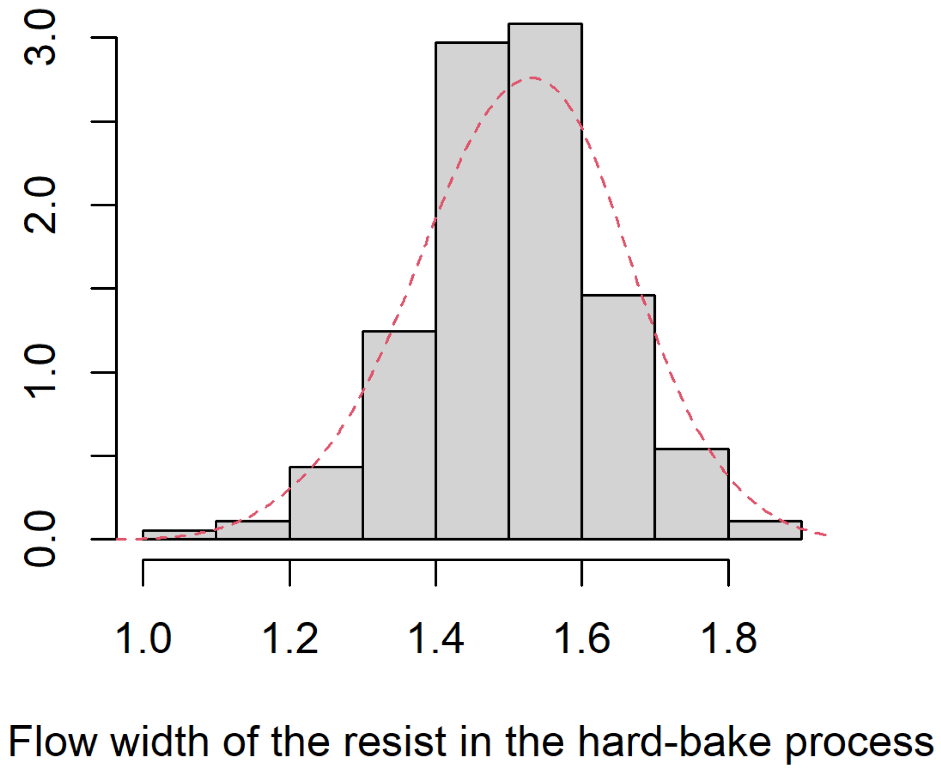
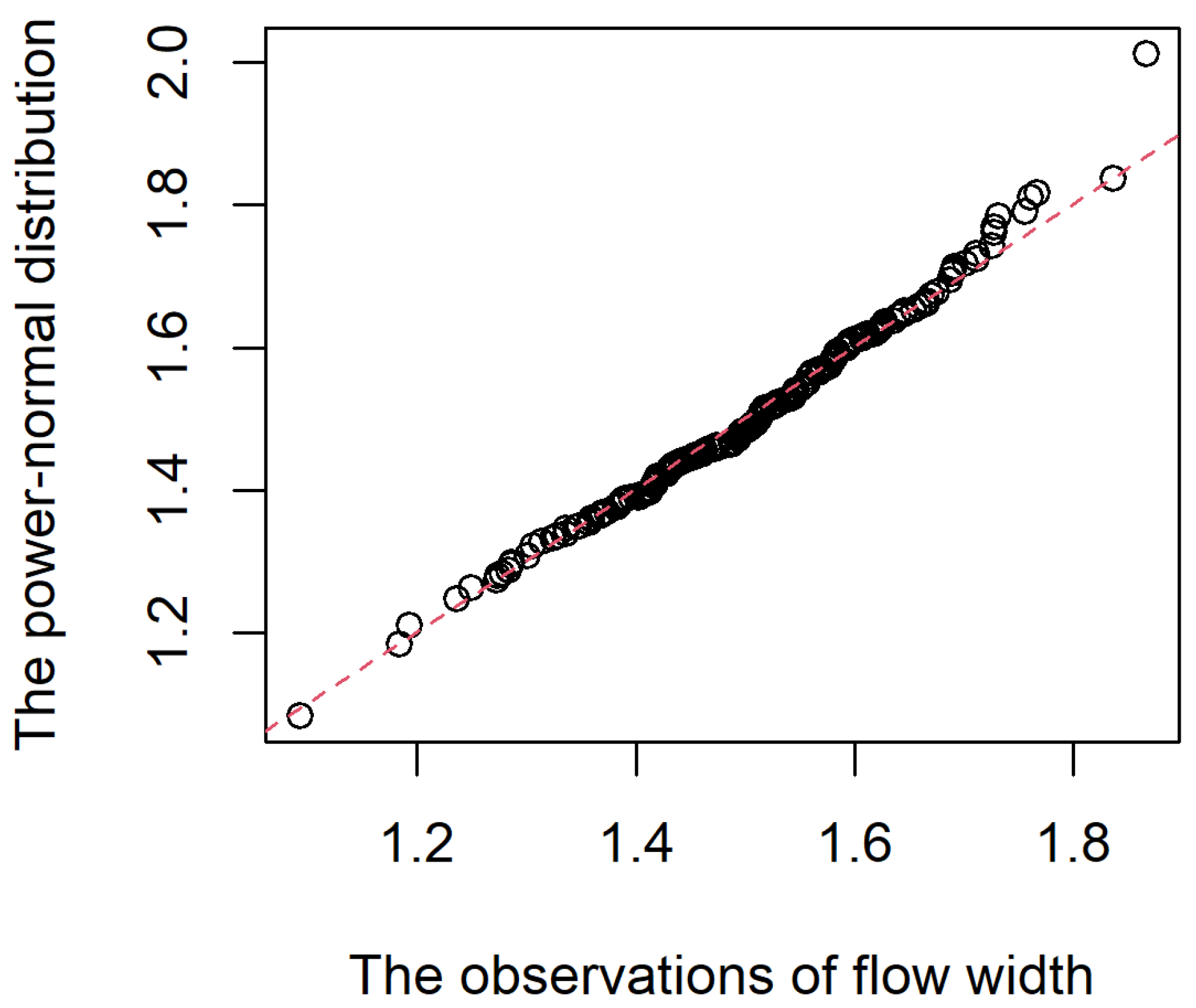
Modeling: Using the proposed maximum likelihood estimation in Section 3.1 with the initial values of ${\xi }_0$, ${\gamma }_0=1$ and ${\sigma }_0$, where ${\xi }_0$ and ${\sigma }_0$ are the sample mean and standard deviation of the data set, respectively. Based on the simulation results in Table 1, a random sample of $n=185$ should be okay to obtain reliable MLEs of the model parameters when $\gamma$ is close to 1. We obtain the MLEs $\widehat{\xi }=1.5282$, $\widehat{\gamma }=0.8015$ and $\widehat{\sigma }=0.1197$ for the power-normal distribution. The dashed line in Figure 2 is the density curve of the power-normal distribution based on the obtained MLEs. We can see that the power-normal distribution has a good fitting to this data set.

The quantile-to-quantile plot based on the flow width data and the power-normal distribution is presented in Figure 3. All the dots are plotted around the straight line. Hence, the quantile-to-quantile plot indicates that the power-normal distribution can be the right model to characterize the flow width data. The test statistic of the Kolmogorov-Smirnov test based on the flow width data and power-normal distribution is $0.062$ with the p-value of $0.2917$. Based on the Kolmogorov-Smirnov test, we conclude that the power-normal distribution can be a good model to characterize the flow width data. Because the MLE of the shape parameter, $\widehat{\gamma }=0.8015$, is closed to 1, this estimate indicates that the distribution of the flow width data has a slightly skewed shape.

Refer to the lower specification limit of $LSL=1$ suggested by [2], we let $L=1$. The MLE of the $C_L$ can be ${\widehat{C}}_L=(1.5282-1)/0.1197=4.4127$. The high value of the ${\widehat{C}}_L$ indicates a good process capability for the flow width of the resist in the hard-bark process. Based on the original sample with 185 observations of flow width, the $95\%$ PBP and BCP confidence intervals of the model parameters and $C_L$ are obtained and reported in

Table 2. The 95% bootstrap confidence intervals based on the original sample with n = 185 observations.

	PBP		BCP
Parameter	Lower Limit	Upper Limit	Lower Limit	Upper Limit
$\xi$	1.2716	1.6886	1.2575	1.6842
$\gamma$	0.0839	5.5656	0.0944	5.9333
$\sigma$	0.0511	0.1932	0.0535	0.1965
$C_L$	1.4040	13.4726	1.2975	12.7272

. We can find that the obtained PBP and BCP intervals for each parameter are close. Two bootstrap intervals of $C_L$ recommend a good quality for the flow width of the resist in the hard-bake manufacturing process due to two lower limits of $C_L$ are significantly larger than 1.

Stage 2:

The impact of the sample size on the quality of the confidence interval of${\mathit{C}}_{\mathit{L}}$: In this stage, 315 observations are generated from the model obtained in Stage 1 to investigate the impact of the sample size on the quality of the PBP and BCP intervals of $C_L$. We merge the original 185 observations with the generated observations. The merged sample has a size of 500. We are interested in studying how much the length of confidence interval can be reduced when the sample size increases. The PBP and BCP confidence intervals of $C_L$ are evaluated based on the first 300 and all 500 observations in the merged sample. All computation results are reported in

Table 3. The 95% bootstrap confidence intervals based on the merged sample with $n=300$ and 500.

		PBP		BCP
$\mathit{n}$	Parameter	Lower Limit	Upper Limit	Lower Limit	Upper Limit
300	$\xi$	1.4302	1.6886	1.1832	1.5994
	$\gamma$	0.1089	1.8209	0.3820	5.4131
	$\sigma$	0.0588	0.1512	0.0925	0.2001
	$C_L$	2.8738	11.7485	0.9781	6.3928
500	$\xi$	1.4595	1.6634	1.2955	1.5825
	$\gamma$	0.1902	1.5053	0.4523	4.1516
	$\sigma$	0.0734	0.1453	0.0975	0.1784
	$C_L$	3.1750	9.0023	1.6642	5.8747

.

From Table 3 we can find that the lengths of PBP and BCP confidence intervals are reduced when the sample size increases. Both the PBP and BCP methods are competitive for estimating $\xi$, $\sigma$ and $C_L$. The PBP method outperforms the BCP method to estimate $\gamma$ with a shorter length of confidence interval. Table 3 also indicates the quality of the PBP, and BCP methods can be significantly improved when the sample size increases. The BCP method significantly outperforms the PBP method for evaluating the $C_L$ in terms of the length of confidence interval.

6. Concluding Remarks

In this study, we proposed a maximum likelihood estimation procedure to obtain the MLEs of the model parameters and PPI. Moreover, the approximate confidence intervals of the model parameters and PPI are obtained based on the parametric bootstrap methods of PBP and BCP. The exact Fisher information matrix is derived and we study the weakness of using the exact Fisher information matrix to obtain an approximate confidence interval for the model parameters and PPI. Monte Carlo simulations were conducted to evaluate the quality of the proposed methods. We find that a sample with 250 or 300 is large enough to obtain the reliable MLEs of the model parameters and PPI. An example about the flow width of the resist in a hard-bake process of integrated circuit is used to illustrate the applications of the proposed methods.

The maximum likelihood estimation procedure and the bootstrap method of BCP ask a big sample for the power-normal distribution to obtain reliable point and interval estimation results. Bias-correction methods could be helpful to improve the performance of the proposed maximum likelihood estimation procedure. In the case of small samples, finding other reliable parameter estimation methods with good estimation performance is an important issue. Moreover, establishing inference methods with censoring schemes also are an important issue for the power-normal distribution. All these topics will be studied in the near future.

References

1. Pan, J.; Wu, S. Process capability analysis for non-normal relay test data. Microelectron. Reliab. 1997, 37, 421–428. [Google Scholar] [CrossRef]
2. Montgomery, D.C. Statistical Quality Control: A Modern Introduction, 7th ed.; John Wiley & Sons: New York, NY, USA, 2012. [Google Scholar]
3. Hong, C.-W.; Wu, J.-W.; Cheng, C.-H. A look at the Burr and related distribution. Appl. Math. Comput. 2007, 184, 336–350. [Google Scholar]
4. Lee, H.-M.; Wu, J.-W.; Lei, C.-L.; Hung, W.L. Implementing lifetime performance index of products with two-parameter exponential distribution. Int. J. Syst. Sci. 2011, 42, 1305–1321. [Google Scholar] [CrossRef]
5. Wu, S.-F.; Chiu, C.-J. Computational testing algorithmic procedure of assessment for lifetime performance index of products with two-parameter exponential distribution based on the multiply type II censored sample. J. Stat. Comput. Simul. 2014, 84, 2016–2122. [Google Scholar] [CrossRef]
6. Wu, S.-F.; Lin, Y.-P. Computational testing algorithmic procedure of assessment for lifetime performance index of products with one-parameter exponential distribution under progressive type I interval censoring. Math. Comput. Simul. 2016, 120, 79–90. [Google Scholar] [CrossRef]
7. Lee, W.-C.; Wu, J.-W.; Hong, C.-W. Assessing the lifetime performance index of products from progressively type II right censored data using Burr XII model. Math. Comput. Simul. 2009, 79, 2167–2179. [Google Scholar] [CrossRef]
8. Ahmadi, M.V.; Doostparast, M.; Ahmadi, J. Statistical inference for the lifetime performance index based on generalised order statistics from exponential distribution. Int. J. Syst. Sci. 2009, 46, 1094–1107. [Google Scholar] [CrossRef]
9. Lee, W.-C.; Wu, J.-W.; Hong, M.-L. Assessing the lifetime performance index of Rayleigh products based on the Bayesian estimation under progressive type II right censored samples. J. Comput. Appl. Math. 2011, 235, 1676–1688. [Google Scholar] [CrossRef]
10. Ahmadi, M.V.; Doostparast, M.; Ahmadi, J. Estimating the lifetime performance index with Weibull distribution based on progressive first-failure censoring scheme. J. Comput. Appl. Math. 2013, 239, 93–102. [Google Scholar] [CrossRef]
11. Goto, M.; Inoue, T. Some properties of power-normal distribution. Jpn. J. Biom. 1980, 1, 28–54. [Google Scholar] [CrossRef]
12. Goto, M.; Inoue, T.; Tsuchiya, Y. On estimation of parameters in power-normal distribution. Bull. Inform. Cybern. 1984, 21, 41–53. [Google Scholar] [CrossRef]
13. Goto, M.; Matsubara, Y.; Tsuchiya, Y. Power-normal distribution and its applications. Rep. Stat. Appl. Res. 1983, 30, 8–28. [Google Scholar]
14. Freeman, J.; Modarres, R. Inverse Box-Cox: The power-normal distribution. Stat. Probab. Lett. 2006, 76, 764–772. [Google Scholar] [CrossRef]
15. Castillo, N.O.; Gallardo, D.I.; Bolfarine, H.; Gómez, H. Truncated power-normal distribution with application to non-negative measurements. Entropy 2018, 433, 433. [Google Scholar] [CrossRef] [Green Version]
16. Maruo, K.; Goto, M. Percentile estimation based on the power-normal distribution. Comput. Stat. 2013, 28, 241–356. [Google Scholar] [CrossRef]
17. Gupta, R.D.; Gupta, R.C. Analyzing skewed data by power normal model. Test 2008, 17, 197–210. [Google Scholar] [CrossRef]
18. Maruo, K.; Shirahata, S.; Goto, M. Underlying assumptions of the power-normal distribution. Behaviormetrika 2011, 38, 85–95. [Google Scholar] [CrossRef]
19. Azzalini, A. A class of distributions which includes the normal ones. Scand. J. Stat. 1985, 12, 171–178. [Google Scholar]
20. Efron, B.; Tibshirani, R.J. An Introduction to the Bootstrap; Chapman & Hall: New York, NY, USA, 1993. [Google Scholar]
21. Lio, Y.L.; Tsai, T.-R.; Chiang, J.-Y. Estimation of the lower confidence limit of the breaking strength percentiles under progressive type-II censoring. J. Chin. Inst. Ind. Eng. 2012, 29, 16–29. [Google Scholar] [CrossRef]
22. Dey, S.; Saha, M.; Maiti, S.S.; Jun, C.-H. Bootstrap confidence intervals of generalized process capability index Cpyk for for Lindley and power Lindley distributions. Commun. Stat.-Simul. Comput. 2018, 47, 249–262. [Google Scholar] [CrossRef]
23. Besseris, G.J. Evaluation of robust scale estimators for modified Weibull process capability indices and their bootstrap confidence intervals. Comput. Ind. Eng. 2019, 128, 135–149. [Google Scholar] [CrossRef]
24. Park, C.; Dey, S.; Ouyang, L.; Byun, J.-H.; Leeds, M. Improved bootstrap confidence intervals for the process capability index Cpk. Commun. Stat.-Simul. Comput. 2020, 49, 2583–2603. [Google Scholar] [CrossRef]
Figure 1. The CRs for estimating ξ , γ , σ , and C L through using the PBP and BCP methods. The dashed line is the nominal value.
Mathematics 10 00035 g001
Figure 2. The histogram of the flow width data in Example 1.
Mathematics 10 00035 g002
Figure 3. The histogram of the flow width data in Example 1.
Mathematics 10 00035 g003