Abstract
The present paper proposes a five-dimensional mathematical model for studying the labor market, focusing on unemployment, migration, fixed term contractors, full time employment and the number of available vacancies. The distributed time delay is considered in the rate of change of available vacancies that depends on the past regular employment levels. The non-dimensional mathematical model is introduced and the existence of the equilibrium points is analyzed. The positivity and boundedness of solutions are provided and global asymptotic stability findings are presented both for the employment free equilibrium and the positive equilibrium. The numerical simulations support the theoretical results.
1. Introduction
Over the time, one of the many challenges that a country faces is economical downturn fuelled by unemployment. The causes of appearance of this phenomena are countless and are based on country specificity. Problems ranging from the increasing population to slow economic growth are some of the leading factors linked to unemployment spanning out of control. One of the negative impact of unemployment pertains to the social side that puts the affected population at high risk, such as psychological and mental health problems, just to name a few [1]. Any responsible government cannot ignore the signals coming from the labour market and should take appropriate and immediate actions to improve the overall situation.
Therefore, the need to manage and handle the tendency of unwanted spread of unemployment brings about the necessity of studying the behaviour of complex mathematical models in conjunction with numerical simulations. In order to comprehend the dynamics of unemployment, using some concepts from [2], the following variables have been considered in a previous mathematical model investigated in [3,4]: number of unemployed persons, employed persons and new vacancies; time delay has been incorporated into the rate of change for creation of new vacancies. Moreover, by resorting to the skill development programs, Misra et al. [5] demonstrated the link between the betterment of workers’ capabilities and the reduction of unemployment. The effect of training programs has also been studied in [6]. Furthermore, Harding and Neamţu [7] considered the migration as a contributing factor when defining policies pertaining to unemployment, including distributed time delay. The optimal control analysis has been completed in [8,9].
The motivation of the present paper is centered around the existing mathematical models, enabling the development of new ways for studying unemployment, based on the past history of the state variables. The potential impact of our findings is related to upcoming biological and economical mathematical models connected to population dynamics. The most important benefit could be related to the strategic policy makers of our society.
The novelty of this paper is the investigation of the interaction among the number of unemployed persons, immigrants, temporary employed persons, regularly employed persons and the number of available vacancies, in the set up of delay differential equations. The distributed time delay has been incorporated to reflect the dependence of the rate of change of available vacancies on the past regular employment levels. Basically, this type of delay is highlighted for acquiring the realistic sides of the economic process [10,11,12,13,14,15,16]. It is important to emphasize that there are many mathematical models including distributed time delays, originating from population biology, epidemiology and economics [17,18,19,20,21,22,23,24,25,26,27,28,29,30,31,32,33].
The paper is structured as follows: the mathematical model and its non-dimensional version are introduced in Section 2; the existence of the equilibrium points of the model is discussed in Section 3 and the positivity and boundedness of solutions are proved in Section 4; global asymptotic stability results are proved for the employment free equilibrium and the positive equilibrium in Section 5 and Section 6, respectively; Section 7 includes numerical simulations to highlight the theoretical findings, followed by conclusions which are formulated in Section 8.
2. The Mathematical Model and Its Non-Dimensional Version
We consider the following five variables which describe the mathematical model for to control the unemployment: the number of unemployed persons , the number of immigrants , the number of temporary employed persons , the number of regularly employed persons , respectively and the number of available vacancies at time t.
The system of differential equations is:
where , , , and are positive constants: the constant growth rate of unemployed persons entering the labor market, the rate of hiring, the rate of firing, the rate of move to unemployment, the rate of move to temporary employment; the rate of migration of unemployed persons; is the rate of return or death, the rate of temporary employment, the rate of retirement, migration or death of employed persons; the rate of available vacancies; is the rate of good job finding; represent the exogenous increase in migration, is the migrant employment rate.
The bounded, piecewise continuous function is the delay kernel with average time delay for available vacancies based on past employment levels. Hence, h is a probability density function satisfying the following properties:
With the changes of variables:
system (1) becomes a non-dimensional system, with fewer dimensionless parameters and dimensionless state variables:
where the delay kernel is and the coefficients are expressed as
Initial conditions for system (4) are considered of the form
where belong to the Banach space (where ) of continuous real valued functions defined on such that , considered with respect to the norm:
The existence and uniqueness of solutions, as well as the continuous dependence of solutions on initial conditions, in the framework of the distributed delay system (4), are guaranteed by theoretical results presented in [34].
3. Equilibrium Points of the Model
The equilibrium points are constant solutions of system (4) and hence they satisfy the following algebraic equations:
On one hand, we observe that system (5) has at least one solution, which corresponds to the case when . Hence, we obtain the equilibrium point given by:
where
This equilibrium point corresponds to the state of no regular employment and no available vacancies.
We now introduce the basic reproduction number , which has the role of a threshold parameter that prognosticates whether the unemployment, immigration and temporary employment problems will increase or decrease. Using the next generation matrix method, we deduce:
On the other hand, system (5) has at least one solution with the last component , if and only if is the solution of the following cubic equation:
where
where , and are given above and
In fact, we distinguish two cases:
Case 1: If then and system (4) has at least one positive equilibrum point. Moreover, if either , or and , Descartes’ rule of signs guarantees the existence of a unique positive equilibrium point .
Case 2: If then , we may have either two or zero positive equilibrium points. For instance, if and , system (4) does not have positive equilibrium points.
4. Positivity and Boundedness of Solutions
Theorem 1.
Proof.
As a first step, we will show that the open positive (nonnegative) orthant of is invariant to the flow of system (4). Considering initial conditions , for , based on the continuity of the solutions, there exists such that , for any and any .
In a similar manner, it can be show that , for any .
Moreover, from the first four equations of system (4) we observe that
and taking into account that we have
Therefore, using basic differential inequality techniques, we obtain:
for any
On one hand, if it follows that , for any . Otherwise, if , we have
Solving the last equation of (4) for leads to
Using the generalized l’Hospital rule (see Lemma 1.1 in [35]) in conjunction with Lemma 1 from [4], we deduce:
which concludes the proof. □
5. Global Stability Analysis for
Theorem 2.
The equilibrium point is globally asymptotically stable in the open positive orthant , regardless of the delay kernel , if the following inequality holds:
Proof.
Let us consider an arbitrary solution , , of system (4), with initial conditions . From Theorem 1 it follows that , for any and . Hence, we consider the functions
and we further denote:
Therefore, we have:
Furthermore, we evaluate
and
Moreover, considering
we have:
Further, considering:
we compute
Therefore, as inequality holds, there exists such that . By means of LaSalle’s invariance principle [12,36], we deduce that the equilibrium equilibrium point of system (4) is globally asymptotically stable in . □
6. Global Stability Analysis for
Theorem 3.
The positive equilibrium point is globally asymptotically stable in the open positive orthant , regardless of the delay kernel , if .
Proof.
Let us consider an arbitrary solution , , of system (4), with initial conditions . From Theorem 1 it follows that , for any and .
Taking into account that , for any , we construct the Lyapunov function as follows:
where
and
and we further denote:
With the notations defined above, taking into account that is an equilibrium point of system (4) we have:
Furthermore, we get:
Moreover, we obtain:
and finally:
Furthermore, taking into account the algebraic relations satisfied by the coordinates of the equilibrium point , we obtain:
Denoting and employing the inequality , for any , we have:
Moreover:
Therefore, combining the previous relations, we have:
For , choosing , it follows that:
Jensen’s inequality for probability density functions applied to the concave logarithmic function [37] provides that
and hence, we obtain that , for any . Hence, by means of LaSalle’s invariance principle [12,36], we deduce that the equilibrium equilibrium point of system (4) is globally asymptotically stable in . □
7. Numerical Simulations
7.1. Scenario 1: Global Asymptotic Stability of
In this case, we first consider the following parameter values: , , , , , , , , , , , , . For these parameter values, system (1) has a unique equilibrium point:
We remark that the basic reproduction number satisfies inequality (7), and hence, based on Theorem 2, the equilibrium point is globally asymptotically stable, for any delay kernel considered in system (1).
In fact, in this scenario, the very low hiring rates for unemployed persons, immigrants and temporarily employed persons and the low value of the basic reproduction number, justify the existence of only one globally asymptotically stable equilibrium point, . For the numerical simulations shown in Figure 1, the following initial condition has been considered: , which represents a plausible situation in a stable economic environment. However, due to the low hiring rates mentioned above, the trajectories of system (1) quickly converge to the “crisis” equilibrium , corresponding to no regular employment and no available vacancies.

Figure 1.
Evolution of the state variables , , , and in Scenario 1, with fixed initial conditions: and a discrete time delay ; the trajectories converge to the equilibrium point =(1000, 50, 6000, 0, 0).
7.2. Scenario 2: Global Asymptotic Stability of
For the numerical simulations we considered: , , , , , , , , , , , , . For these values of the parameters, we obtain a unique positive equilibrium point
In fact, in this scenario, we observe that the hiring rate is very small, and hence, global asymptotic stability can be expected for the equilibrium , in line with the theoretical results presented in Theorem 3. Indeed, in the numerical simulations shown in Figure 2, convergence to the positive equilibrium is observed, starting from a “crisis” initial condition: , with almost no regular employment or available vacancies. We emphasize that in this scenario, the convergence is very slow. Moreover, a larger time delay is associated with an even slower convergence to the positive equilibrium.
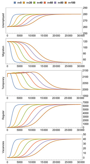
Figure 2.
Evolution of the state variables , , , and in Scenario 2, with initial conditions: and a discrete time delay ; the trajectories converge to .
8. Conclusions
The present paper introduced a five-dimensional mathematical model that facilitates the understanding of new ways for studying the labour market while observing the levels of unemployment, migration, fixed term contractors, full time employment and the number of available vacancies. The distributed time delay has been incorporated to reflect the dependence of the rate of change of available vacancies on the past regular employment levels.
The positivity and boundedness of solutions have been provided. Using the basic reproduction number, the existence of equilibrium points has been discussed. As a consequence, the employment free equilibrium and positive equilibrium came into focus, for which we have undertaken a global stability analysis, regardless of the delay kernel included in the mathematical model.
Through the numerical simulations, the theoretical findings have been emphasized as well, further revealing that in an economic crisis scenario (Scenario 1), a fast convergence to the “crisis” equilibrium (with no regular employment or vacancies) is observed. However, in Scenario 2, if the initial conditions correspond to a crisis situation and the parameters of the system are adjusted, the convergence to the positive equilibrium is very slow, which reflects the slow recovery of the job market.
The findings of the paper could be used as input for future developments linked to population dynamics, and the decision making entities of the society could also use these findings in various strategies.
The proposed mathematical model is open ended that allows the introduction of future variables depicting the effects of the unemployment, such as poverty and unsocial behaviours that can lead to crime, as in [38].
Author Contributions
Conceptualization, E.K., M.N. and L.F.V.; methodology, E.K., M.N. and L.F.V.; software, E.K., M.N. and L.F.V.; validation, E.K., M.N. and L.F.V.; formal analysis, E.K., M.N. and L.F.V.; investigation, E.K., M.N. and L.F.V.; resources, E.K., M.N. and L.F.V.; data curation, E.K., M.N. and L.F.V.; writing—original draft preparation, E.K., M.N. and L.F.V.; writing—review and editing, E.K., M.N. and L.F.V.; visualization, E.K., M.N. and L.F.V.; supervision, E.K., M.N. and L.F.V.; project administration, E.K., M.N. and L.F.V.; funding acquisition, E.K., M.N. and L.F.V. All authors have read and agreed to the published version of the manuscript.
Funding
This research received no external funding.
Institutional Review Board Statement
Not applicable.
Informed Consent Statement
Not applicable.
Data Availability Statement
Not applicable.
Conflicts of Interest
The authors declare no conflict of interest.
References
- Singh, A.K.; Singh, P.K.; Misra, A.K. Combating unemployment through skill development. Nonlinear Anal. Model. Control 2020, 25, 919–937. [Google Scholar] [CrossRef]
- Nikolopoulos, C.; Tzanetis, D. A model for housing allocation of a homeless population due to a natural disaster. Nonlinear Anal. Real. World Appl. 2003, 4, 561–579. [Google Scholar] [CrossRef]
- Misra, A.; Singh, A.K. A delay mathematical model for the control of unemployment. Differ. Equations Dyn. Syst. 2013, 21, 291–307. [Google Scholar] [CrossRef]
- Kaslik, E.; Neamţu, M.; Vesa, L.F. Global stability analysis of an unemployment model with distributed delay. Math. Comput. Simul. 2021, 185, 535–546. [Google Scholar] [CrossRef]
- Misra, A.; Singh, A.K.; Singh, P.K. Modeling the Role of Skill Development to Control Unemployment. In Differential Equations and Dynamical Systems; Springer Nature: Cham, Switzerland, 2017; pp. 1–13. [Google Scholar]
- Al-Maalwi, R.; Al-Sheikh, S.; Ashi, H.; Asiri, S. Mathematical modeling and parameter estimation of unemployment with the impact of training programs. Math. Comput. Simul. 2021, 182, 705–720. [Google Scholar] [CrossRef]
- Harding, L.; Neamţu, M. A dynamic model of unemployment with migration and delayed policy intervention. Comput. Econ. 2018, 51, 427–462. [Google Scholar] [CrossRef]
- Munoli, S.; Gani, S.; Gani, S. A Mathematical Approach to Employment Policies: An Optimal Control Analysis. Int. J. Stat. Syst. 2017, 12, 549–565. [Google Scholar]
- Mallick, U.; Biswas, M. Optimal Analysis of Unemployment Model taking Policies to Control. Adv. Model. Optim. 2018, 20, 303–312. [Google Scholar]
- Corduneanu, C.; Lakshmikantham, V. Equations with unbounded delay: A survey. Nonlinear Anal. Theory Methods Appl. 1980, 4, 831–877. [Google Scholar] [CrossRef]
- Gripenberg, G.; Londen, S.O.; Staffans, O. Volterra Integral and Functional Equations; Cambridge University Press: Cambridge, UK, 1990; Volume 34. [Google Scholar]
- Hale, J.K.; Lunel, S.M.V. Introduction to Functional Differential Equations; Applied Mathematical Sciences; Springer: New York, NY, USA, 1991; Volume 99. [Google Scholar]
- Hino, Y.; Murakami, S.; Naito, T. Functional Differential Equations with Infinite Delay; Lecture Notes in Mathematics Series; Springer: New York, NY, USA, 1991; Volume 1473. [Google Scholar]
- Diekmann, O.; Van Gils, S.A.; Lunel, S.M.; Walther, H.O. Delay Equations: Functional-, Complex-, and Nonlinear Analysis; Applied Mathematical Sciences; Springer: New York, NY, USA, 1995; Volume 110. [Google Scholar]
- Diekmann, O.; Gyllenberg, M. Equations with infinite delay: Blending the abstract and the concrete. J. Differ. Equ. 2012, 252, 819–851. [Google Scholar] [CrossRef]
- Staffans, O.J. Hopf bifurcation for functional and functional differential equations with infinite delay. J. Differ. Equ. 1987, 70, 114–151. [Google Scholar] [CrossRef][Green Version]
- Kuang, Y. Delay Differential Equations: With Applications in Population Dynamics; Academic Press: New York, NY, USA, 1993; Volume 1913. [Google Scholar]
- Liu, S.; Chen, L. Necessary-sufficient conditions for permanence and extinction in Lotka-Volterra system with distributed delays. Appl. Math. Lett. 2003, 16, 911–917. [Google Scholar] [CrossRef]
- Adimy, M.; Crauste, F.; Halanay, A.; Neamţu, M.; Opriş, D. Stability of limit cycles in a pluripotent stem cell dynamics model. Chaos Solitons Fractals 2006, 27, 1091–1107. [Google Scholar] [CrossRef][Green Version]
- Berezansky, L.; Braverman, E.; Idels, L. Nicholson’s blowflies differential equations revisited: Main results and open problems. Appl. Math. Model. 2010, 34, 1405–1417. [Google Scholar] [CrossRef]
- Cushing, J.M. Integrodifferential Equations and Delay Models in Population Dynamics; Springer Science & Business Media: Berlin/Heidelberg, Germany, 2013; Volume 20. [Google Scholar]
- Huang, G.; Liu, A. A note on global stability for a heroin epidemic model with distributed delay. Appl. Math. Lett. 2013, 26, 687–691. [Google Scholar] [CrossRef]
- Chen, S.S.; Cheng, C.Y.; Takeuchi, Y. Stability analysis in delayed within-host viral dynamics with both viral and cellular infections. J. Math. Anal. Appl. 2016, 442, 642–672. [Google Scholar] [CrossRef]
- Liu, Q.; Jiang, D. Stationary distribution and extinction of a stochastic predator–prey model with distributed delay. Appl. Math. Lett. 2018, 78, 79–87. [Google Scholar] [CrossRef]
- Bichara, D.M. Global analysis of multi-host and multi-vector epidemic models. J. Math. Anal. Appl. 2019, 475, 1532–1553. [Google Scholar] [CrossRef] [PubMed]
- Hallegatte, S.; Ghil, M.; Dumas, P.; Hourcade, J.C. Business cycles, bifurcations and chaos in a neo-classical model with investment dynamics. J. Econ. Behav. Organ. 2008, 67, 57–77. [Google Scholar] [CrossRef]
- Matsumoto, A.; Szidarovszky, F. Delay differential nonlinear economic models. In Nonlinear Dynamics in Economics, Finance and Social Sciences; Springer: Berlin/Heidelberg, Germany, 2010; pp. 195–214. [Google Scholar]
- Matsumoto, A.; Szidarovszky, F. Delay differential neoclassical growth model. J. Econ. Behav. Organ. 2011, 78, 272–289. [Google Scholar] [CrossRef]
- Yu, J.; Peng, M. Stability and bifurcation analysis for the Kaldor-Kalecki model with a discrete delay and a distributed delay. Phys. A Stat. Mech. Appl. 2016, 460, 66–75. [Google Scholar] [CrossRef]
- Fanelli, V.; Maddalena, L. A nonlinear dynamic model for credit risk contagion. Math. Comput. Simul. 2020, 174, 45–58. [Google Scholar] [CrossRef]
- Chen, W.; Wu, W.; Teng, Z. Complete dynamics in a nonlocal dispersal two-strain SIV epidemic model with vaccinations and latent delays. Appl. Comput. Math. 2020, 19, 360–391. [Google Scholar]
- Khalsaraei, M.M.; Shokri, A.; Ramos, H.; Heydari, S. A positive and elementary stable nonstandard explicit scheme for a mathematical model of the influenza disease. Math. Comput. Simul. 2021, 182, 397–410. [Google Scholar] [CrossRef]
- Shokri, A.; Khalsaraei, M.M.; Molayi, M. Dynamically Consistent NSFD Methods for Predator-prey System. J. Appl. Comput. Mech. 2021, 25, 1565–1574. [Google Scholar]
- Kolmanovskii, V.; Myshkis, A. Introduction to the Theory and Applications of Functional Differential Equations; Kluwer Academic Publishers: Dordrecht, The Netherlands, 1999; Volume 463. [Google Scholar]
- Manojlovic, J.; Maric, V. An asymptotic analysis of positive solutions of Thomas-Fermi type sublinear differential equations. Mem. Differ. Equ. Math. Phys 2012, 57, 75–94. [Google Scholar]
- Smith, H.L. An Introduction to Delay Differential Equations with Applications to the Life Sciences; Springer New York: New York, NY, USA, 2011; Volume 57. [Google Scholar]
- Durrett, R. Probability: Theory and Examples; Cambridge University Press: Cambridge, UK, 2019; Volume 49. [Google Scholar]
- Soemarsono, A.; Fitria, I.; Nugraheni, K.; Hanifa, N. Analysis of Mathematical Model on Impact of Unemployment Growth to Crime Rates. Journal of Physics: Conference Series; IOP Publishing: Bristol, UK, 2021; Volume 1726, p. 012003. [Google Scholar] [CrossRef]
Publisher’s Note: MDPI stays neutral with regard to jurisdictional claims in published maps and institutional affiliations. |
© 2021 by the authors. Licensee MDPI, Basel, Switzerland. This article is an open access article distributed under the terms and conditions of the Creative Commons Attribution (CC BY) license (https://creativecommons.org/licenses/by/4.0/).