Bipolar Complex Fuzzy Hamacher Aggregation Operators and Their Applications in Multi-Attribute Decision Making

Abstract

On the basis of Hamacher operations, in this manuscript, we interpret bipolar complex fuzzy Hamacher weighted average (BCFHWA) operator, bipolar complex fuzzy Hamacher ordered weighted average (BCFHOWA) operator, bipolar complex fuzzy Hamacher hybrid average (BCFHHA) operator, bipolar complex fuzzy Hamacher weighted geometric (BCFHWG) operator, bipolar complex fuzzy Hamacher ordered weighted geometric (BCFHOWG) operator, and bipolar complex fuzzy Hamacher hybrid geometric (BCFHHG) operator. We present the features and particular cases of the above-mentioned operators. Subsequently, we use these operators for methods that can resolve bipolar complex fuzzy multiple attribute decision making (MADM) issues. We provide a numerical example to authenticate the interpreted methods. In the end, we compare our approach with existing methods in order to show its effectiveness and practicality.

1. Introduction

In classical set theory (CST), we have only two possibilities, yes or no, i.e., an item either belongs to a set or does not. This means that the characteristic function of an item can give values $0$ or $1$. The CST fails in many situations such as age, intelligence, and height. To overcome this issue, Zadeh [1] presented the idea of the fuzzy set (FS). In FS theory, the membership degree (MD) belongs to the closed interval $\left[0, 1\right]$ instead of $\left\{0, 1\right\}$. Mardani et al. [2] presented decision-making (DM) methods based on fuzzy aggregation operators. Merigó and Casanovas [3] described fuzzy generalized hybrid aggregation operators and their application in fuzzy DM. FS theory only considers MD, but in various circumstances, we need a non-membership degree (NMD). To handle such problems, Atanassov [4] provided the notion of intuitionistic FS (IFS) denoted by an MD and NMD with the condition that the sum of MD and NMD belongs to the closed interval $\left[0, 1\right]$. Xu [5] introduced intuitionistic fuzzy (IF) aggregation operators. The generalized IF aggregation operators are based on confidence levels for group DM given by Rahman et al. [6]. Verma and Merigó [7] presented multiple-attribute group DM (MAGDM) based on two-dimensional linguistic IF aggregation operators. Huang [8] defined the IF Hamacher aggregation operators and their application to MADM. Garg [9] presented IF Hamacher aggregation operators’ entropy weight and their applications to multi-criteria DM (MCDM) issues.

Subsequently, the bipolar fuzzy set (BFS) [10,11] has risen as another technique that illustrates vagueness in MADM issues. The BFS is denoted by the pair of positive degree PD, whose range is $\left[0, 1\right]$, and by negative degree (ND), whose range is the $\left[-1, 0\right]$. Lee [12] presented a comparison of interval-valued FS, IFSs, and bipolar valued FSs. BFSs have been applied in several research zones such as bipolar logical cognitive and set theory [13,14], graph theory [15,16], quantum computing [17,18], traditional Chinese medicine notions [19,20], physics and philosophy [21], and biosystem regulation [22]. Gul [23] presented the bipolar fuzzy (BF) aggregation operators. Wei et al. [24] presented BF Hamacher aggregation operators in MADM. BF Dombi aggregation operators and their application in MADM are given by Jana et al. [25]. Jana et al. [26] described BF Dombi prioritized aggregation operators in MADM. Riaz and Tehrim [27] presented a robust extension of VIKOR method for BFSs in which they use connection numbers of SPA theory-based metric spaces. Sarwar et al. [28] defined the DM approach on the basis of competition graphs and extended the TOPSIS method under the BF environment. A new notion of the bipolar soft set was presented by Mahmood [29]. Abdullah et al. [30] described the BF soft sets and their applications in DM issues.

Motivated by the extension of a real number to a complex number, Ramot et al. [31] extended the range of FS from the closed interval $\left[0, 1\right]$ to the unit disc in a complex plane. They named this extension complex FS (CFS), which can be represented in a polar structure, i.e., ${ℱ}_{\mathfrak{J}}\left(\tau \right)=r_{\mathfrak{J}}\left(\tau \right)e^{\mathfrak{i} {\theta }_{\mathfrak{J}}\left(\tau \right)}$, where $r_{\mathfrak{J}}\left(\tau \right)\in \left[0, 1\right]$ and $0\le {\theta }_{\mathfrak{J}}\left(\tau \right)\le 2\pi$. Complex fuzzy information can be visualized with the assistance of hypergraphs [32]. Later, Tamir et al. [33] described CFS by changing the range from a unit disc (polar structure) to a unit square with a cartesian structure, i.e., ${ℱ}_{\mathfrak{J}}\left(\tau \right)={\eta }_{\mathfrak{J}}\left(\tau \right) + \mathfrak{i} {\sigma }_{\mathfrak{J}}\left(\tau \right)$, where ${\eta }_{\mathfrak{J}}\left(\tau \right), {\sigma }_{\mathfrak{J}}\left(\tau \right)\in \left[0, 1\right]$. Yazdanbakhsh and Dick [34] described a systematic review of CFSs. Tamir et al. [35] presented CFSs and complex fuzzy (CF) logic as an overview of the theory. Dagher [36] presented a complex fuzzy c-means algorithm. Bi et al. [37] interpreted CF geometric aggregation operators. The CF power aggregation operators were given by Hu et al. [38]. Bi et al. [39] described CF arithmetic aggregation operators. Garg and Rani [40] described innovative aggregation operators and ranking methods for complex IFSs. Mahmood et al. [41] presented the idea of complex hesitant FSs. Behera and Chakraverty [42] produced a novel procedure for solving real and CF systems. The notion of complex dual hesitant FS was presented by Ur Rehman et al. [43]. Ma et al. [44] interpreted CFS with applications in signals.

Mahmood and Ur Rehman [45] presented a bipolar complex fuzzy set (BCFS). The theory of BCFS has a powerful structure in the shape of complex numbers whose real and unreal terms are belonging to unit intervals. The BCFS is used in many real-life situations: for example, consider that a mayor considers whether he should start a new public transport program in a city. For this purpose, he hires an expert who assesses the given possibilities. The expert must have considered four important aspects of this program, that is, the positive aspects or effects (i.e., people’s benefits), the negative aspects or side effects (i.e., the city’s extra economic costs), and society’s positive and negative responses to the project. For example, an expert rates $0.6$ points to the positive aspect, $-0.4$ to the negative aspect, $0.7$ to society’s positive response, and $-0.5$ to society’s negative response. To handle this type of data, the expert must use BCFS, since no other existing structure can manage this kind of information. The principle of FSs, BFSs, and CFSs are the particular cases of the novel BCFS, and many individuals have employed it in the region of different circumstances. However, to date, the theory of BCFS has had no implementation in the region of decision-making, medical diagnosis, pattern recognition, image segmentation, and analysis of carcinoma. Additionally, Hamacher t-norm and t-conorm are the most important techniques to be employed in the region of FS, BFS, and CFS. The particularities of this analysis consist of implementing Hamacher t-norm and t-conorm in the environment of BCFS and discussing their important cases. Hamacher aggregation operator generalizes the ordinary t-norm and t-conorm through the parameter. For example, if we take the parameter equal to 1, then the Hamacher t-norm and t-conorm will be narrowed to the ordinary t-norm and t-conorm, respectively. On the other hand, if we take the parameter equal to 2, the Hamacher t-norm and t-conorm will be narrowed to the Einstein t-norm and t-conorm, respectively.

In this manuscript, we invented BCFHWA, BCFHOWA, BCFHHA BCFHWG, BCFHOWG, and BCFHHG operators and discuss their particular cases. The benefits of implementation of Hamacher aggregation operators in the setting of BCFSs comprise the prevailing theories such as FS, BFS, and CFS. We can obtain particular cases such as bipolar fuzzy averaging and bipolar fuzzy geometric aggregation operator by taking the parameter 1 in the bipolar complex Hamacher aggregation operator. Similarly, we obtain Einstein averaging and Einstein geometric aggregation operators by taking the parameter equal to 2. This shows that the Hamacher t-norm and t-conorm are powerful due to parameters involved in the operation of Hamacher t-norm and t-conorm.

The remaining article is organized in the following way: In Section 2, we review the elementary definitions such as FS, BFS, CFS, and BCFS. In Section 3 of this article, the basic operations, score function, and accuracy function of the BCFS are given. In Section 4, we have three subsections: in the first subsection, we introduce the Hamacher operations of BCFSs; in the second subsection, we present bipolar complex fuzzy Hamacher arithmetic aggregation (BCFHAA) operators; and in the third subsection, we present bipolar complex fuzzy Hamacher geometric aggregation (BCFHGA) operators. In Section 5 of this article, we present the MADM technique based on the interpreted bipolar complex Hamacher aggregation operators in Section 4 under the BCFS setting. In Section 6, we develop a practical MADM case to explain the application of the interpreted operators. In Section 7, we make a comparative study of our method and of the existing methods so as to show the authenticity and superiority of our approach. In Section 8, we draw our final conclusions.

2. Preliminaries

In this section, we shortly analyze several basic results linked to FSs, BFSs, CFSs, and BCFS. Let ${\rm T}$ be universal set throughout in this article.

Definition 1 

([1]). A FS has the structure $\mathfrak{J}=\left\{\left(\tau , {\eta }_{\mathfrak{J}}\right) | \tau \in {\rm T}\right\}$ on ${\rm T}$, where ${\eta }_{\mathfrak{J}}:{\rm T}\to \left[0, 1\right]$ implies the membership degree (MD) of every element $\tau \in {\rm T}$. Let $FS$ be the identification of the set of all fuzzy numbers (FNs), and if $\mathfrak{J}\in FS$, then $\mathfrak{J}={\eta }_{\mathfrak{J}}$.

Definition 2 

([10,11]). A BFS has the structure $\mathfrak{J}=\left\{\left(\tau , {\eta }_{\mathfrak{J}}^{+}, {\eta }_{\mathfrak{J}}^{-}\right) | \tau \in {\rm T}\right\}$ on ${\rm T}$, where ${\eta }_{\mathfrak{J}}^{+}:{\rm T}\to \left[0, 1\right]$ implies the PD, and ${\eta }_{\mathfrak{J}}^{-}:{\rm T}\to \left[-1, 0\right]$ implies the ND. Let $BFS$ be the identification of the set of all bipolar FNs (BFNs), and if $\mathfrak{J}\in BFN$, then $\mathfrak{J}=\left({\eta }_{\mathfrak{J}}^{+}, {\eta }_{\mathfrak{J}}^{-}\right)$.

Definition 3 

([33]). A CFS has the structure $\mathfrak{J}=\left\{\left(\tau , {ℱ}_{\mathfrak{J}}\right) | \tau \in {\rm T}\right\}=\left\{\left(\tau ,{\eta }_{\mathfrak{J}} + \mathfrak{i} {\sigma }_{\mathfrak{J}}\right) | \tau \in {\rm T}\right\}$ on a ${\rm T}$, where ${ℱ}_{\mathfrak{J}}\left(\tau \right)$ is a complex MD, which gives the values in a unit square of a complex plane, ${\eta }_{\mathfrak{J}}, {\sigma }_{\mathfrak{J}}\in \left[0, 1\right]$, and $\mathfrak{i}=\sqrt{-1}$. Let $CFS$ be the identification of the set of all complex FNs (CFNs), and if $\mathfrak{J}\in CFN$, then $\mathfrak{J}=\left({\eta }_{\mathfrak{J}}+\mathfrak{i} {\sigma }_{\mathfrak{J}}\right)$.

Definition 4 

([45]). A BCFS $\mathfrak{J}$ is denoted by a positive degree (PD) ${ℱ}_{\mathfrak{J}}^{+}$and a negative degree (ND)${ℱ}_{\mathfrak{J}}^{-}$, which are assigned to every elemen $\tau$ of ${\rm T}$. The values of ${ℱ}_{\mathfrak{J}}^{+}$and${ℱ}_{\mathfrak{J}}^{-}$ may obtain all values that lie within the unit square in a complex plane and are of the shape ${ℱ}_{\mathfrak{J}}^{+}={\eta }_{\mathfrak{J}}^{+}+\mathfrak{i} {\sigma }_{\mathfrak{J}}^{+}$ and ${ℱ}_{\mathfrak{J}}^{-}={\eta }_{\mathfrak{J}}^{-}+\mathfrak{i} {\sigma }_{\mathfrak{J}}^{-}$, where ${\eta }_{\mathfrak{J}}^{+},{\sigma }_{\mathfrak{J}}^{+}\in \left[0, 1\right]$ and ${\eta }_{\mathfrak{J}}^{-},{\sigma }_{\mathfrak{J}}^{-}\in \left[-1, 0\right]$. A BCFS is of the form

$$\mathfrak{J}=\left\{\left(\tau , {ℱ}_{\mathfrak{J}}^{+}, {ℱ}_{\mathfrak{J}}^{-}\right) | \tau \in {\rm T}\right\}$$

(1)

where ${ℱ}_{\mathfrak{J}}^{+}:{\rm T}\to \left\{x+\mathfrak{i} 𝔂 | x, 𝔂\in \left[0, 1\right]\right\}$ and ${ℱ}_{\mathfrak{J}}^{-}:{\rm T}\to \left\{x+\mathfrak{i} 𝓎 | x, 𝓎\in \left[-1, 0\right]\right\}$.

Let$BCFS$be the identification of the set of all bipolar CFNs (BCFNs), and if$\mathfrak{J}\in BCFN$, then$\mathfrak{J}=\left({ℱ}_{\mathfrak{J}}^{+}, {ℱ}_{\mathfrak{J}}^{-}\right)=\left({\eta }_{\mathfrak{J}}^{+}+\mathfrak{i} {\sigma }_{\mathfrak{J}}^{+}, {\eta }_{\mathfrak{J}}^{-}+\mathfrak{i} {\sigma }_{\mathfrak{J}}^{-}\right)$.

Definition 5 

([46]). Hamacher product ${\otimes }_H$ and Hamacher sum ${\oplus }_H$ are t-norm and t-conorm respectively, given as

For any${\tau }_1, {\tau }_2\in \left[0, 1\right]$, $\alpha >0$

$${\tau }_1{\otimes }_H{\tau }_2=\frac{{\tau }_1{\tau }_2}{\alpha +\left(1-\alpha \right)\left({\tau }_1+{\tau }_2-{\tau }_1{\tau }_2\right)}$$

(2)

$${\tau }_1{\oplus }_H{\tau }_2=\frac{\left({\tau }_1+{\tau }_2-{\tau }_1{\tau }_2\right)-\left(1-\alpha \right){\tau }_1{\tau }_2}{1-\left(1-\alpha \right){\tau }_1{\tau }_2}$$

(3)

3. Elementary Operations Based on BCFS

This section introduces the basic operations, the scoring function, and the accuracy function of the BCFS.

Definition 6. 

The score function${\mathcal{S}}_B\left(\mathfrak{J}\right):{\rm T}\to \left[0, 1\right]$of a BCFN$\mathfrak{J}=\left({ℱ}_{\mathfrak{J}}^{+}, {ℱ}_{\mathfrak{J}}^{-}\right)=\left({\eta }_{\mathfrak{J}}^{+}+\mathfrak{i} {\sigma }_{\mathfrak{J}}^{+}, {\eta }_{\mathfrak{J}}^{-}+\mathfrak{i}{\sigma }_{\mathfrak{J}}^{-}\right)$is defined as

$${\mathcal{S}}_B\left(\mathfrak{J}\right)=\frac{1}{4}\left(2+{\eta }_{\mathfrak{J}}^{+}+{\sigma }_{\mathfrak{J}}^{+}+{\eta }_{\mathfrak{J}}^{-}+{\sigma }_{\mathfrak{J}}^{-}\right)$$

(4)

Definition 7. 

The accuracy function${\mathscr{H}}_B\left(\mathfrak{J}\right):{\rm T}\to \left[0, 1\right]$of a BCFN$\mathfrak{J}=\left({ℱ}_{\mathfrak{J}}^{+}, {ℱ}_{\mathfrak{J}}^{-}\right)=\left({\eta }_{\mathfrak{J}}^{+}+\mathfrak{i} {\sigma }_{\mathfrak{J}}^{+}, {\eta }_{\mathfrak{J}}^{-}+\mathfrak{i}{\sigma }_{\mathfrak{J}}^{-}\right)$is defined as

$${\mathscr{H}}_B\left(\mathfrak{J}\right)=\frac{{\eta }_{\mathfrak{J}}^{+}+{\sigma }_{\mathfrak{J}}^{+}-{\eta }_{\mathfrak{J}}^{-}-{\sigma }_{\mathfrak{J}}^{-}}{4}$$

(5)

      It is obvious that${\mathcal{S}}_B\left(\mathfrak{J}\right)\in \left[0, 1\right]$and${\mathscr{H}}_B\left(\mathfrak{J}\right)\in \left[0, 1\right]$. Observe that${\mathscr{H}}_B\left(\mathfrak{J}\right)$evaluates the accuracy degree of$\mathfrak{J}$. The greatest value of${\mathscr{H}}_B\left(\mathfrak{J}\right)$implies the greatest accuracy degree of the BCFN$\mathfrak{J}$.

Definition 8. 

For two BCFNs$\mathfrak{J}=\left({ℱ}_{\mathfrak{J}}^{+}, {ℱ}_{\mathfrak{J}}^{-}\right)$and$\mathfrak{K}=\left(\left({ℱ}_{\mathfrak{K}}^{+}, {ℱ}_{\mathfrak{K}}^{-}\right)\right)$, we introduce the order relation$\succ$as$\mathfrak{J}\succ \mathfrak{K}$if and only if

• ${\mathcal{S}}_B\left(\mathfrak{J}\right)>{\mathcal{S}}_B\left(\mathfrak{K}\right)$
  or
• ${\mathcal{S}}_B\left(\mathfrak{J}\right)={\mathcal{S}}_B\left(\mathfrak{K}\right)$ and ${\mathscr{H}}_B\left(\mathfrak{J}\right)>{\mathscr{H}}_B\left(\mathfrak{K}\right)$
  or
• ${\mathcal{S}}_B\left(\mathfrak{J}\right)={\mathcal{S}}_B\left(\mathfrak{K}\right)$ and ${\mathscr{H}}_B\left(\mathfrak{J}\right)={\mathscr{H}}_B\left(\mathfrak{K}\right)$

Definition 9. 

In BCFN notation, let be any two BCFS$\mathfrak{J}=\left({ℱ}_{\mathfrak{J}}^{+}, {ℱ}_{\mathfrak{J}}^{-}\right)=\left({\eta }_{\mathfrak{J}}^{+}+\mathfrak{i} {\sigma }_{\mathfrak{J}}^{+}, {\eta }_{\mathfrak{J}}^{-}+\mathfrak{i} {\sigma }_{\mathfrak{J}}^{-}\right)$and$\mathfrak{K}=\left( {ℱ}_{\mathfrak{K}}^{+}, {ℱ}_{\mathfrak{K}}^{-}\right)=\left({\eta }_{\mathfrak{K}}^{+}+\mathfrak{i} {\sigma }_{\mathfrak{K}}^{+}, {\eta }_{\mathfrak{K}}^{-}+\mathfrak{i}{\sigma }_{\mathfrak{K}}^{-}\right)$. Then, operations on BCFSs$\mathfrak{J}$, $\mathfrak{K}$are described as follows:

• $\mathfrak{J}\oplus \mathfrak{K}=\left(\left({\eta }_{\mathfrak{J}}^{+}{\oplus }_H{\eta }_{\mathfrak{K}}^{+}\right)+\mathfrak{i} \left({\sigma }_{\mathfrak{J}}^{+}{\oplus }_H {\sigma }_{\mathfrak{K}}^{+}\right),-\left(\left|{\eta }_{\mathfrak{J}}^{-}\right|{\otimes }_H\left|{\eta }_{\mathfrak{K}}^{-}\right|\right)-\mathfrak{i} \left(\left|{\sigma }_{\mathfrak{J}}^{-}\right|{\otimes }_H\left|{\sigma }_{\mathfrak{K}}^{-}\right|\right)\right)$
• $\mathfrak{J}\otimes \mathfrak{K}=\left(\left({\eta }_{\mathfrak{J}}^{+}{\otimes }_H{\eta }_{\mathfrak{K}}^{+}\right)+\mathfrak{i} \left({\sigma }_{\mathfrak{J}}^{+}{\otimes }_H {\sigma }_{\mathfrak{K}}^{+}\right),-\left(\left|{\eta }_{\mathfrak{J}}^{-}\right|{\oplus }_H\left|{\eta }_{\mathfrak{K}}^{-}\right|\right)-\mathfrak{i} \left(\left|{\sigma }_{\mathfrak{J}}^{-}\right|{\oplus }_H\left|{\sigma }_{\mathfrak{K}}^{-}\right|\right)\right)$
• $\lambda \mathfrak{J}=\left({\oplus }_H^{\lambda }\left({\eta }_{\mathfrak{J}}^{+}\right)+\mathfrak{i} {\oplus }_H^{\lambda }\left({\sigma }_{\mathfrak{J}}^{+}\right),-{\otimes }_H^{\lambda }\left(\left|{\eta }_{\mathfrak{J}}^{-}\right|\right)-\mathfrak{i} {\oplus }_H^{\lambda }\left(\left|{\sigma }_{\mathfrak{J}}^{-}\right|\right)\right)$
• ${\mathfrak{J}}^{\lambda }=\left({\otimes }_H^{\lambda }\left({\eta }_{\mathfrak{J}}^{+}\right)+\mathfrak{i} {\otimes }_H^{\lambda }\left({\sigma }_{\mathfrak{J}}^{+}\right),-{\otimes }_H^{\lambda }\left(\left|{\eta }_{\mathfrak{J}}^{-}\right|\right)-\mathfrak{i}{\oplus }_H^{\lambda }\left(\left|{\sigma }_{\mathfrak{J}}^{-}\right|\right)\right)$

For$\alpha =1$, Definition 9, after substituting formulas from Definition 5, takes the of the form of the following Definition 10.

Definition 10.For two BCFNs$=\left({ℱ}_{\mathfrak{J}}^{+}, {ℱ}_{\mathfrak{J}}^{-}\right)=\left({\eta }_{\mathfrak{J}}^{+}+\mathfrak{i} {\sigma }_{\mathfrak{J}}^{+}, {\eta }_{\mathfrak{J}}^{-}+\mathfrak{i} {\sigma }_{\mathfrak{J}}^{-}\right)$ $\mathfrak{K}=\left( {ℱ}_{\mathfrak{K}}^{+}, {ℱ}_{\mathfrak{K}}^{-}\right)=\left({\eta }_{\mathfrak{K}}^{+}+\mathfrak{i} {\sigma }_{\mathfrak{K}}^{+}, {\eta }_{\mathfrak{K}}^{-}+\mathfrak{i}{\sigma }_{\mathfrak{K}}^{-}\right)$, and for any real number$\lambda >0$, we introduce the following operations:

• $\mathfrak{J}\oplus \mathfrak{K}=\left(\begin{array}{c}{\eta }_{\mathfrak{J}}^{+}+{\eta }_{\mathfrak{K}}^{+}-{\eta }_{\mathfrak{J}}^{+}{\eta }_{\mathfrak{K}}^{+}+\mathfrak{i}\left( {\sigma }_{\mathfrak{J}}^{+}+{\sigma }_{\mathfrak{K}}^{+}-{\sigma }_{\mathfrak{J}}^{+} {\sigma }_{\mathfrak{K}}^{+}\right), \\ -\left({\eta }_{\mathfrak{J}}^{-}{\eta }_{\mathfrak{K}}^{-}\right)+\mathfrak{i} \left(-\left({\sigma }_{\mathfrak{J}}^{-}{\sigma }_{\mathfrak{K}}^{-}\right)\right)\end{array}\right)$;
• $\mathfrak{J}\otimes \mathfrak{K}=\left(\begin{array}{c}{\eta }_{\mathfrak{J}}^{+}{\eta }_{\mathfrak{K}}^{+}+\mathfrak{i} {\sigma }_{\mathfrak{J}}^{+} {\sigma }_{\mathfrak{K}}^{+}, \\ {\eta }_{\mathfrak{J}}^{-}+{\eta }_{\mathfrak{K}}^{-}+{\eta }_{\mathfrak{J}}^{-}{\eta }_{\mathfrak{K}}^{-}+\mathfrak{i} \left({\sigma }_{\mathfrak{J}}^{-}+{\sigma }_{\mathfrak{K}}^{-}+{\sigma }_{\mathfrak{J}}^{-}{\sigma }_{\mathfrak{K}}^{-}\right)\end{array}\right)$;
• $\lambda \mathfrak{J}=\left(1-{\left(1-{\eta }_{\mathfrak{J}}^{+}\right)}^{\lambda }+\mathfrak{i} \left(1-{\left(1-{\sigma }_{\mathfrak{J}}^{+}\right)}^{\lambda }\right),-{\left|{\eta }_{\mathfrak{J}}^{-}\right|}^{\lambda }+\mathfrak{i} \left(-{\left|{\sigma }_{\mathfrak{J}}^{-}\right|}^{\lambda }\right) \right)$;
• ${\mathfrak{J}}^{\lambda }=\left({\eta }_{\mathfrak{J}}^{+}{}^{\lambda }+\mathfrak{i} {\sigma }_{\mathfrak{J}}^{+}{}^{\lambda },-1+{\left(1+{\eta }_{\mathfrak{J}}^{-}\right)}^{\lambda }+\mathfrak{i} \left(-1+{\left(1+{\sigma }_{\mathfrak{J}}^{-}\right)}^{\lambda }\right)\right)$;

Theorem 1. 

For BCFNs $\mathfrak{J}=\left({ℱ}_{\mathfrak{J}}^{+}, {ℱ}_{\mathfrak{J}}^{-}\right)=\left({\eta }_{\mathfrak{J}}^{+}+\mathfrak{i} {\sigma }_{\mathfrak{J}}^{+}, {\eta }_{\mathfrak{J}}^{-}+\mathfrak{i} {\sigma }_{\mathfrak{J}}^{-}\right)$, $\mathfrak{K}=\left( {ℱ}_{\mathfrak{K}}^{+}, {ℱ}_{\mathfrak{K}}^{-}\right)=\left({\eta }_{\mathfrak{K}}^{+}+\mathfrak{i} {\sigma }_{\mathfrak{K}}^{+}, {\eta }_{\mathfrak{K}}^{-}+\mathfrak{i}{\sigma }_{\mathfrak{K}}^{-}\right)$, and $\mathfrak{L}=\left( {ℱ}_{\mathfrak{L}}^{+}, {ℱ}_{\mathfrak{L}}^{-}\right)=\left({\eta }_{\mathfrak{L}}^{+}+\mathfrak{i} {\sigma }_{\mathfrak{L}}^{+}, {\eta }_{\mathfrak{L}}^{-}+\mathfrak{i}{\sigma }_{\mathfrak{L}}^{-}\right)$, and for real numbers $\lambda , {\lambda }_1, {\lambda }_2>0$, the following holds:

• $\mathfrak{J}\oplus \mathfrak{K}=\mathfrak{K}\oplus \mathfrak{J}$
• $\mathfrak{J}\otimes \mathfrak{K}=\mathfrak{K}\otimes \mathfrak{J}$
• $\lambda \left(\mathfrak{J}\oplus \mathfrak{K}\right)=\lambda \mathfrak{J}\oplus \lambda \mathfrak{K}$
• ${\left(\mathfrak{J}\otimes \mathfrak{K}\right)}^{\lambda }={\mathfrak{J}}^{\lambda }\otimes {\mathfrak{K}}^{\lambda }$
• ${\lambda }_1\mathfrak{J}\oplus {\lambda }_2\mathfrak{J}=\left({\lambda }_1+{\lambda }_2\right)\mathfrak{J}$
• ${\mathfrak{J}}^{{\lambda }_1}\otimes {\mathfrak{J}}^{{\lambda }_2}={\mathfrak{J}}^{{\lambda }_1+{\lambda }_2}$
• ${\left({\mathfrak{J}}^{{\lambda }_1}\right)}^{{\lambda }_2}={\mathfrak{J}}^{{\lambda }_1{\lambda }_2}$.
• $\mathfrak{J}\oplus \left(\mathfrak{K}\oplus \mathfrak{L}\right)=\left(\mathfrak{J}\oplus \mathfrak{K}\right)\oplus \mathfrak{L}$
• $\mathfrak{J}\otimes \left(\mathfrak{K}\otimes \mathfrak{L}\right)=\left(\mathfrak{J}\otimes \mathfrak{K}\right)\otimes \mathfrak{L}$
• ${\lambda }_1\left({\lambda }_2\mathfrak{J}\right)=\left({\lambda }_1{\lambda }_2\right)\mathfrak{J}$

Proof. 

Trivial. □

4. Bipolar Complex Fuzzy Hamacher Aggregation Operators

In this section, we have two subsections. We present BCFHAA operators in the first subsection and BCFHGA operators in the second subsection.

4.1. Bipolar Complex Fuzzy Hamacher Arithmetic Aggregation Operators

In this subsection, we present the bipolar complex fuzzy Hamacher weighted average (BCFHWA) operator and bipolar complex fuzzy Hamacher ordered weighted average (BCFHOWA) operator. Consider $\mathsf{{\rm K}}$ to be the collection of all BCFNs in this article.

In Definition 11, we invent the BCFHWA operator.

Definition 11. 

The BCFHWA operator is a function from${{\rm K}}^n$to${\rm K}$, i.e.,$BCFHWA:{{\rm K}}^n\to K$presented as

$$BCFHW{A}_{\varpi }\left({\mathfrak{J}}_1, {\mathfrak{J}}_2, {\mathfrak{J}}_3, \dots , {\mathfrak{J}}_n\right)=\begin{array}{c}n\\ \oplus \\ p=1\end{array}\left({\varpi }_p{\mathfrak{J}}_p\right)$$

(6)

where$\varpi ={\left({\varpi }_1, {\varpi }_2,{\varpi }_3,\dots , {\varpi }_n\right)}^{\mathcal{T}}$signifies the weight vector linked with${\mathfrak{J}}_p\left(p=1, 2, \dots , n\right)$and${\varpi }_p\in \left[0, 1\right]$,${\displaystyle \sum }_{p=1}^n{\varpi }_p=1$.

Theorem 2. 

The BCFHWA operator gives a BCFN and

$$\begin{gathered} BCFHW{A}_{\varpi }\left({\mathfrak{J}}_1, {\mathfrak{J}}_2, {\mathfrak{J}}_3, \dots , {\mathfrak{J}}_n\right)=\begin{array}{c}n\\ \oplus \\ p=1\end{array}\left({\varpi }_p{\mathfrak{J}}_p\right) \\ =\left(\begin{array}{c}\frac{\left(\begin{array}{c}{{\displaystyle \prod }}_{p=1}^n{\left(1+\left(\alpha -1\right){\eta }_{{\mathfrak{J}}_p}^{+}\right)}^{{\varpi }_p}\\ -{{\displaystyle \prod }}_{p=1}^n{\left(1-{\eta }_{{\mathfrak{J}}_p}^{+}\right)}^{{\varpi }_p}\end{array}\right)}{\left(\begin{array}{c}{{\displaystyle \prod }}_{p=1}^n{\left(1+\left(\alpha -1\right){\eta }_{{\mathfrak{J}}_p}^{+}\right)}^{{\varpi }_p}+\\ \left(\alpha -1\right){{\displaystyle \prod }}_{p=1}^n{\left(1-{\eta }_{{\mathfrak{J}}_p}^{+}\right)}^{{\varpi }_p}\end{array}\right)}+\mathfrak{i}\frac{\left(\begin{array}{c}{{\displaystyle \prod }}_{p=1}^n{\left(1+\left(\alpha -1\right){\sigma }_{{\mathfrak{J}}_p}^{+}\right)}^{{\varpi }_p}\\ -{{\displaystyle \prod }}_{p=1}^n{\left(1-{\sigma }_{{\mathfrak{J}}_p}^{+}\right)}^{{\varpi }_p}\end{array}\right)}{\left(\begin{array}{c}{{\displaystyle \prod }}_{p=1}^n{\left(1+\left(\alpha -1\right){\sigma }_{{\mathfrak{J}}_p}^{+}\right)}^{{\varpi }_p}+\\ \left(\alpha -1\right){{\displaystyle \prod }}_{p=1}^n{\left(1-{\sigma }_{{\mathfrak{J}}_p}^{+}\right)}^{{\varpi }_p}\end{array}\right)},\\ \frac{-\alpha {{\displaystyle \prod }}_{p=1}^n{\left|{\eta }_{{\mathfrak{J}}_p}^{-}\right|}^{{\varpi }_p}}{\left(\begin{array}{c}{{\displaystyle \prod }}_{p=1}^n{\left(1+\left(\alpha -1\right)\left(1+{\eta }_{{\mathfrak{J}}_p}^{-}\right)\right)}^{{\varpi }_p}\\ +\left(\alpha -1\right){{\displaystyle \prod }}_{p=1}^n{\left|{\eta }_{{\mathfrak{J}}_p}^{-}\right|}^{{\varpi }_p}\end{array}\right)}+\mathfrak{i} \frac{-\alpha {{\displaystyle \prod }}_{p=1}^n{\left|{\sigma }_{{\mathfrak{J}}_p}^{-}\right|}^{{\varpi }_p}}{\left(\begin{array}{c}{{\displaystyle \prod }}_{p=1}^n{\left(1+\left(\alpha -1\right)\left(1+{\sigma }_{{\mathfrak{J}}_p}^{-}\right)\right)}^{{\varpi }_p}\\ +\left(\alpha -1\right){{\displaystyle \prod }}_{p=1}^n{\left|{\sigma }_{{\mathfrak{J}}_p}^{-}\right|}^{{\varpi }_p}\end{array}\right)}\end{array}\right) \end{gathered}$$

(7)

The proof of this theorem is presented in Appendix A.

It can be easily demonstrated that the BCFHWA operator satisfies the following three properties.

Idempotency is an extremely helpful property in various circumstances, as it implies that an operation can be rehashed or revised as frequently as vital without initiating accidental impacts. In the following theorem, we invent the idempotency for the BCFHWA operator.

Theorem 3. 

(Idempotency) If all${\mathfrak{J}}_p\left(p=1, 2, 3, \dots , n\right)$are identical, that is,${\mathfrak{J}}_p=\mathfrak{J} \forall p$, then

$$BCFHW{A}_{\varpi }\left({\mathfrak{J}}_1, {\mathfrak{J}}_2, {\mathfrak{J}}_3, \dots , {\mathfrak{J}}_m\right)=\mathfrak{J}$$

(8)

The proof of this theorem is presented in Appendix A.

The invented BCFHWA operator satisfies the boundedness property, which is interpreted as below.

Theorem 4. 

(Boundedness) Let${\mathfrak{J}}^{-}=\underset{p}{\min {\mathfrak{J}}_p}$, ${\mathfrak{J}}^{+}=\underset{p}{\max {\mathfrak{J}}_p}$. Then

$${\mathfrak{J}}^{-}\preccurlyeq BCFHW{A}_{\varpi }\left({\mathfrak{J}}_1, {\mathfrak{J}}_2, {\mathfrak{J}}_3, \dots , {\mathfrak{J}}_m\right)\preccurlyeq {\mathfrak{J}}^{+}$$

(9)

Monotonicity is a significant trademark in numerous applications. The term comes from monotonic mathematical operations, also called non-decreasing function. In the following theorem, we invent monotonicity for the BCFHWA operator.

Theorem 5. 

(Monotonicity) Let${\mathfrak{J}}_p=\left({ℱ}_{{\mathfrak{J}}_p}^{+}, {ℱ}_{{\mathfrak{J}}_p}^{-}\right)=\left({\eta }_{{\mathfrak{J}}_p}^{+}+\mathfrak{i} {\sigma }_{{\mathfrak{J}}_p}^{+}\left(\tau \right), {\eta }_{{\mathfrak{J}}_p}^{-}+\mathfrak{i} {\sigma }_{{\mathfrak{J}}_p}^{-}\right)\left(p=1, 2, 3, \dots , n\right)$and${\mathfrak{K}}_p=\left({ℱ}_{{\mathfrak{K}}_p}^{+}, {ℱ}_{{\mathfrak{K}}_p}^{-}\right)=\left({\eta }_{{\mathfrak{K}}_p}^{+}+\mathfrak{i} {\sigma }_{{\mathfrak{K}}_p}^{+}\left(\tau \right), {\eta }_{{\mathfrak{K}}_p}^{-}+\mathfrak{i} {\sigma }_{{\mathfrak{K}}_p}^{-}\right)\left(p=1, 2, 3, \dots , n\right)$be two collection of BCFNs. If${\eta }_{{\mathfrak{J}}_p}^{+}\le {\eta }_{{\mathfrak{K}}_p}^{+}$,${\sigma }_{{\mathfrak{J}}_p}^{+}\le {\sigma }_{{\mathfrak{K}}_p}^{+}$ ${\eta }_{{\mathfrak{J}}_p}^{-}\le {\eta }_{{\mathfrak{K}}_p}^{-}$and${\sigma }_{{\mathfrak{J}}_p}^{-}\le {\sigma }_{{\mathfrak{K}}_p}^{-}$for all$p$. Then

$$BCFHW{A}_{\varpi }\left({\mathfrak{J}}_1, {\mathfrak{J}}_2, {\mathfrak{J}}_3, \dots , {\mathfrak{J}}_n\right)\preccurlyeq BCFHW{A}_{\varpi }\left({\mathfrak{K}}_1, {\mathfrak{K}}_2, {\mathfrak{K}}_3, \dots , {\mathfrak{K}}_n\right)$$

(10)

Particular Cases 1. 

We examine two particular cases of the$BCFHWA$operators as follows:

1.

When we take$\alpha =1$, then the $BCFHWA$operator transforms into the bipolar complex fuzzy weighted average (BCFWA) operator

$$\begin{gathered} BCFW{A}_{\varpi }\left({\mathfrak{J}}_1, {\mathfrak{J}}_2, {\mathfrak{J}}_3, \dots , {\mathfrak{J}}_n\right)=\begin{array}{c}n\\ \oplus \\ p=1\end{array}\left({\varpi }_p{\mathfrak{J}}_p\right) \\ =\left(\begin{array}{c}1-{\displaystyle \prod _{p=1}^n}{\left(1-{\eta }_{{\mathfrak{J}}_p}^{+}\right)}^{{\varpi }_p}+\mathfrak{i} 1-{\displaystyle \prod _{p=1}^n}{\left(1-{\sigma }_{{\mathfrak{J}}_p}^{+}\right)}^{{\varpi }_p} ,\\ -{\displaystyle \prod _{p=1}^n}{\left|{\eta }_{{\mathfrak{J}}_p}^{-}\right|}^{{\varpi }_p}+\mathfrak{i} \left(-{\displaystyle \prod _{p=1}^n}{\left|{\sigma }_{{\mathfrak{J}}_p}^{-}\right|}^{{\varpi }_p}\right)\end{array}\right) \end{gathered}$$

(11)

2.

When we take$\alpha =2$, then the BCFHWA operator transforms into the bipolar complex fuzzy Einstein weighted average (BCFEWA) operator

$$\begin{gathered} BCFEW{A}_{\varpi }\left({\mathfrak{J}}_1, {\mathfrak{J}}_2, {\mathfrak{J}}_3, \dots , {\mathfrak{J}}_n\right)=\begin{array}{c}n\\ \oplus \\ p=1\end{array}\left({\varpi }_p{\mathfrak{J}}_p\right) \\ =\left(\begin{array}{c}\frac{\left(\begin{array}{c}{{\displaystyle \prod }}_{p=1}^n{\left(1+{\eta }_{{\mathfrak{J}}_p}^{+}\right)}^{{\varpi }_p}\\ -{{\displaystyle \prod }}_{p=1}^n{\left(1-{\eta }_{{\mathfrak{J}}_p}^{+}\right)}^{{\varpi }_p}\end{array}\right)}{\left(\begin{array}{c}{{\displaystyle \prod }}_{p=1}^n{\left(1+{\eta }_{{\mathfrak{J}}_p}^{+}\right)}^{{\varpi }_p}+\\ {{\displaystyle \prod }}_{p=1}^n{\left(1-{\eta }_{{\mathfrak{J}}_p}^{+}\right)}^{{\varpi }_p}\end{array}\right)}+\mathfrak{i}\frac{\left(\begin{array}{c}{{\displaystyle \prod }}_{p=1}^n{\left(1+{\sigma }_{{\mathfrak{J}}_p}^{+}\right)}^{{\varpi }_p}\\ -{{\displaystyle \prod }}_{p=1}^n{\left(1-{\sigma }_{{\mathfrak{J}}_p}^{+}\right)}^{{\varpi }_p}\end{array}\right)}{\left(\begin{array}{c}{{\displaystyle \prod }}_{p=1}^n{\left(1+{\sigma }_{{\mathfrak{J}}_p}^{+}\right)}^{{\varpi }_p}+\\ {{\displaystyle \prod }}_{p=1}^n{\left(1-{\sigma }_{{\mathfrak{J}}_p}^{+}\right)}^{{\varpi }_p}\end{array}\right)},\\ \frac{-2{{\displaystyle \prod }}_{p=1}^n{\left|{\eta }_{{\mathfrak{J}}_p}^{-}\right|}^{{\varpi }_p}}{\left(\begin{array}{c}{{\displaystyle \prod }}_{p=1}^n{\left(2+{\eta }_{{\mathfrak{J}}_p}^{-}\right)}^{{\varpi }_p}\\ +{{\displaystyle \prod }}_{p=1}^n{\left|{\eta }_{{\mathfrak{J}}_p}^{-}\right|}^{{\varpi }_p}\end{array}\right)}+\mathfrak{i} \frac{-2{{\displaystyle \prod }}_{p=1}^n{\left|{\sigma }_{{\mathfrak{J}}_p}^{-}\right|}^{{\varpi }_p}}{\left(\begin{array}{c}{{\displaystyle \prod }}_{p=1}^n{\left(2+{\sigma }_{{\mathfrak{J}}_p}^{-}\right)}^{{\varpi }_p}\\ +{{\displaystyle \prod }}_{p=1}^n{\left|{\sigma }_{{\mathfrak{J}}_p}^{-}\right|}^{{\varpi }_p}\end{array}\right)}\end{array}\right) \end{gathered}$$

(12)

In the following Definition 12, we invent the BCFHOWA operator.

Definition 12. 

The bipolar complex fuzzy Hamacher ordered weighted average (BCFHOWA) operator is given as

$$BCFHOW{A}_{\varpi }\left({\mathfrak{J}}_1, {\mathfrak{J}}_2, {\mathfrak{J}}_3, \dots , {\mathfrak{J}}_n\right)=\begin{array}{c}n\\ \oplus \\ p=1\end{array}\left({\varpi }_p{\mathfrak{J}}_{\varphi \left(p\right)}\right)$$

(13)

where$\left(\varphi \left(1\right), \varphi \left(2\right), \dots , \varphi \left(n\right)\right)$is a permutation of$\left(1, 2, 3, \dots , n\right)$, such that${\mathfrak{J}}_{\varphi \left(p-1\right)}\ge {\mathfrak{J}}_{\varphi \left(p\right)} \forall p=1, 2, 3, \dots , n$, and$\varpi ={\left({\varpi }_1, {\varpi }_2, {\varpi }_3, \dots , {\varpi }_n\right)}^{\mathcal{T}}$signifies the weight vector linked with${\mathfrak{J}}_p\left(p=1, 2, \dots , n\right)$and${\varpi }_p\in \left[0, 1\right]$,${\displaystyle \sum }_{p=1}^n{\varpi }_p=1$.

Theorem 6. 

The BCFHOWA operator gives a BCFN and

$$\begin{gathered} BCFHOW{A}_{\varpi }\left({\mathfrak{J}}_1, {\mathfrak{J}}_2, {\mathfrak{J}}_3, \dots , {\mathfrak{J}}_n\right)=\begin{array}{c}n\\ \oplus \\ p=1\end{array}\left({\varpi }_p{\mathfrak{J}}_{\varphi \left(p\right)}\right) \\ =\left(\begin{array}{c}\frac{\left(\begin{array}{c}{{\displaystyle \prod }}_{p=1}^n{\left(1+(\alpha -1){\eta }_{{\mathfrak{J}}_{\varphi \left(p\right)}}^{+}\right)}^{{\varpi }_p}\\ -{{\displaystyle \prod }}_{p=1}^n{\left(1-{\eta }_{{\mathfrak{J}}_{\varphi \left(p\right)}}^{+}\right)}^{{\varpi }_p}\end{array}\right)}{\left(\begin{array}{c}{{\displaystyle \prod }}_{p=1}^n{\left(1+(\alpha -1){\eta }_{{\mathfrak{J}}_{\varphi \left(p\right)}}^{+}\right)}^{{\varpi }_p}+\\ (\alpha -1){{\displaystyle \prod }}_{p=1}^n{\left(1-{\eta }_{{\mathfrak{J}}_{\varphi \left(p\right)}}^{+}\right)}^{{\varpi }_p}\end{array}\right)}+\mathfrak{i}\frac{\left(\begin{array}{c}{{\displaystyle \prod }}_{p=1}^n{\left(1+(\alpha -1){\sigma }_{{\mathfrak{J}}_{\varphi \left(p\right)}}^{+}\right)}^{{\varpi }_p}\\ -{{\displaystyle \prod }}_{p=1}^n{\left(1-{\sigma }_{{\mathfrak{J}}_{\varphi \left(p\right)}}^{+}\right)}^{{\varpi }_p}\end{array}\right)}{\left(\begin{array}{c}{{\displaystyle \prod }}_{p=1}^n{\left(1+(\alpha -1){\sigma }_{{\mathfrak{J}}_{\varphi \left(p\right)}}^{+}\right)}^{{\varpi }_p}+\\ (\alpha -1){{\displaystyle \prod }}_{p=1}^n{\left(1-{\sigma }_{{\mathfrak{J}}_{\varphi \left(p\right)}}^{+}\right)}^{{\varpi }_p}\end{array}\right)}\\ \frac{-\alpha {{\displaystyle \prod }}_{p=1}^n{\left|{\eta }_{{\mathfrak{J}}_{\varphi \left(p\right)}}^{-}\right|}^{{\varpi }_p}}{\left(\begin{array}{c}{{\displaystyle \prod }}_{p=1}^n{\left(1+(\alpha -1)(1+{\eta }_{{\mathfrak{J}}_{\varphi \left(p\right)}}^{-}\right)}^{{\varpi }_p}\\ +(\alpha -1){{\displaystyle \prod }}_{p=1}^n{\left|{\eta }_{{\mathfrak{J}}_{\varphi \left(p\right)}}^{-}\right|}^{{\varpi }_p}\end{array}\right)}+\mathfrak{i} \frac{-\alpha {{\displaystyle \prod }}_{p=1}^n{\left|{\sigma }_{{\mathfrak{J}}_{\varphi \left(p\right)}}^{-}\right|}^{{\varpi }_p}}{\left(\begin{array}{c}{{\displaystyle \prod }}_{p=1}^n{\left(1+(\alpha -1)(1+{\sigma }_{{\mathfrak{J}}_{\varphi \left(p\right)}}^{-}\right)}^{{\varpi }_p}\\ +(\alpha -1){{\displaystyle \prod }}_{p=1}^n{\left|{\sigma }_{{\mathfrak{J}}_{\varphi \left(p\right)}}^{-}\right|}^{{\varpi }_p}\end{array}\right)}\end{array}\right) \end{gathered}$$

(14)

Proof. 

The proof is similar to that of Theorem 2. □

One can easily prove that the BCFHOWA operator satisfies the following three properties. Idempotency is an extremely helpful property in various circumstances, since it implies that an operation can be rehashed or revised as frequently as vital without initiating accidental impacts. In the following theorem, we invent the idempotency for the BCFHOWA operator.

Theorem 7. 

(Idempotency) If all${\mathfrak{J}}_p\left(p=1, 2, 3, \dots , n\right)$are identical, that is,${\mathfrak{J}}_p=\mathfrak{J} \forall p$, then

$$BCFHOW{A}_{\varpi }\left({\mathfrak{J}}_1, {\mathfrak{J}}_2, {\mathfrak{J}}_3, \dots , {\mathfrak{J}}_m\right)=\mathfrak{J}$$

(15)

The invented BCFHOWA operator satisfies the boundedness property, which is interpreted as below.

Theorem 8. 

(Boundedness) Let${\mathfrak{J}}^{-}=\underset{p}{\min {\mathfrak{J}}_p}$, ${\mathfrak{J}}^{+}=\underset{p}{\max {\mathfrak{J}}_p}$. Then

$${\mathfrak{J}}^{-}\preccurlyeq BCFHOW{A}_{\varpi }\left({\mathfrak{J}}_1, {\mathfrak{J}}_2, {\mathfrak{J}}_3, \dots , {\mathfrak{J}}_m\right)\preccurlyeq {\mathfrak{J}}^{+}$$

(16)

Monotonicity is a significant trademark in numerous applications. The term comes from monotonic mathematical operations, also called the non-decreasing function. In the following theorem, we invent monotonicity for the BCFHWA operator.

Theorem 9. 

(Monotonicity) Let${\mathfrak{J}}_p=\left({ℱ}_{{\mathfrak{J}}_p}^{+}, {ℱ}_{{\mathfrak{J}}_p}^{-}\right)=\left({\eta }_{{\mathfrak{J}}_p}^{+}+\mathfrak{i} {\sigma }_{{\mathfrak{J}}_p}^{+}\left(\tau \right), {\eta }_{{\mathfrak{J}}_p}^{-}+\mathfrak{i} {\sigma }_{{\mathfrak{J}}_p}^{-}\right)\left(p=1, 2, 3, \dots , n\right)$and${\mathfrak{K}}_p=\left({ℱ}_{{\mathfrak{K}}_p}^{+}, {ℱ}_{{\mathfrak{K}}_p}^{-}\right)=\left({\eta }_{{\mathfrak{K}}_p}^{+}+\mathfrak{i} {\sigma }_{{\mathfrak{K}}_p}^{+}\left(\tau \right), {\eta }_{{\mathfrak{K}}_p}^{-}+\mathfrak{i} {\sigma }_{{\mathfrak{K}}_p}^{-}\right)\left(p=1, 2, 3, \dots , n\right)$be two collection of BCFNs. If${\eta }_{{\mathfrak{J}}_p}^{+}\le {\eta }_{{\mathfrak{K}}_p}^{+}$,${\sigma }_{{\mathfrak{J}}_p}^{+}\le {\sigma }_{{\mathfrak{K}}_p}^{+}$,${\eta }_{{\mathfrak{J}}_p}^{-}\le {\eta }_{{\mathfrak{K}}_p}^{-}$, and${\sigma }_{{\mathfrak{J}}_p}^{-}\le {\sigma }_{{\mathfrak{K}}_p}^{-}$for all$p$. Then

$$BCFHOW{A}_{\varpi }\left({\mathfrak{J}}_1, {\mathfrak{J}}_2, {\mathfrak{J}}_3, \dots , {\mathfrak{J}}_n\right)\preccurlyeq BCFHOW{A}_{\varpi }\left({\mathfrak{K}}_1, {\mathfrak{K}}_2, {\mathfrak{K}}_3, \dots , {\mathfrak{K}}_n\right)$$

(17)

Particular Cases 2. 

We examine two particular cases of the$BCFHOWA$operator as follows:

1.

When we take$\alpha =1$, then the BCFHOWA operator transforms into the bipolar complex fuzzy ordered weighted average (BCFOWA) operator

$$\begin{gathered} BCFW{A}_{\varpi }\left({\mathfrak{J}}_1, {\mathfrak{J}}_2, {\mathfrak{J}}_3, \dots , {\mathfrak{J}}_n\right)=\begin{array}{c}n\\ \oplus \\ p=1\end{array}\left({\varpi }_p{\mathfrak{J}}_{\varphi \left(p\right)}\right) \\ =\left(\begin{array}{c}1-{\displaystyle \prod }_{p=1}^n{\left(1-{\eta }_{{\mathfrak{J}}_{\varphi \left(p\right)}}^{+}\right)}^{{\varpi }_p}+\mathfrak{i} 1-{\displaystyle \prod }_{p=1}^n{\left(1-{\sigma }_{{\mathfrak{J}}_{\varphi \left(p\right)}}^{+}\right)}^{{\varpi }_p} ,\\ -{\displaystyle \prod }_{p=1}^n{\left|{\eta }_{{\mathfrak{J}}_{\varphi \left(p\right)}}^{-}\right|}^{{\varpi }_p}+\mathfrak{i} \left(-{\displaystyle \prod }_{p=1}^n{\left|{\sigma }_{{\mathfrak{J}}_{\varphi \left(p\right)}}^{-}\right|}^{{\varpi }_p}\right)\end{array}\right) \end{gathered}$$

(18)

2.

When we take$\alpha =2$, then the BCFHOWA operator transforms into the bipolar complex fuzzy Einstein ordered weighted average (BCFEOWA) operator

$$\begin{gathered} BCFEW{A}_{\varpi }\left({\mathfrak{J}}_1, {\mathfrak{J}}_2, {\mathfrak{J}}_3, \dots , {\mathfrak{J}}_n\right)=\begin{array}{c}n\\ \oplus \\ p=1\end{array}\left({\varpi }_p{\mathfrak{J}}_{𝝓\left(p\right)}\right) \\ =\left(\begin{array}{c}\frac{\left(\begin{array}{c}{{\displaystyle \prod }}_{p=1}^n{\left(1+{\eta }_{{\mathfrak{J}}_{𝝓\left(p\right)}}^{+}\right)}^{{\varpi }_p}\\ -{{\displaystyle \prod }}_{p=1}^n{\left(1-{\eta }_{{\mathfrak{J}}_{𝝓\left(p\right)}}^{+}\right)}^{{\varpi }_p}\end{array}\right)}{\left(\begin{array}{c}{{\displaystyle \prod }}_{p=1}^n{\left(1+{\eta }_{{\mathfrak{J}}_{𝝓\left(p\right)}}^{+}\right)}^{{\varpi }_p}+\\ {{\displaystyle \prod }}_{p=1}^n{\left(1-{\eta }_{{\mathfrak{J}}_{𝝓\left(p\right)}}^{+}\right)}^{{\varpi }_p}\end{array}\right)}+\mathfrak{i}\frac{\left(\begin{array}{c}{{\displaystyle \prod }}_{p=1}^n{\left(1+{\sigma }_{{\mathfrak{J}}_{𝝓\left(p\right)}}^{+}\right)}^{{\varpi }_p}\\ -{{\displaystyle \prod }}_{p=1}^n{\left(1-{\sigma }_{{\mathfrak{J}}_{𝝓\left(p\right)}}^{+}\right)}^{{\varpi }_p}\end{array}\right)}{\left(\begin{array}{c}{{\displaystyle \prod }}_{p=1}^n{\left(1+{\sigma }_{{\mathfrak{J}}_{𝝓\left(p\right)}}^{+}\right)}^{{\varpi }_p}+\\ {{\displaystyle \prod }}_{p=1}^n{\left(1-{\sigma }_{{\mathfrak{J}}_{𝝓\left(p\right)}}^{+}\right)}^{{\varpi }_p}\end{array}\right)}\\ \frac{-2{{\displaystyle \prod }}_{p=1}^n{\left|{\eta }_{{\mathfrak{J}}_{𝝓\left(p\right)}}^{-}\right|}^{{\varpi }_p}}{\left(\begin{array}{c}{{\displaystyle \prod }}_{p=1}^n{\left(2+{\eta }_{{\mathfrak{J}}_{𝝓\left(p\right)}}^{-}\right)}^{{\varpi }_p}\\ +{{\displaystyle \prod }}_{p=1}^n{\left|{\eta }_{{\mathfrak{J}}_{𝝓\left(p\right)}}^{-}\right|}^{{\varpi }_p}\end{array}\right)}+\mathfrak{i} \frac{-2{{\displaystyle \prod }}_{p=1}^n{\left|{\sigma }_{{\mathfrak{J}}_{𝝓\left(p\right)}}^{-}\right|}^{{\varpi }_p}}{\left(\begin{array}{c}{{\displaystyle \prod }}_{p=1}^n{\left(2+{\sigma }_{{\mathfrak{J}}_{𝝓\left(p\right)}}^{-}\right)}^{{\varpi }_p}\\ + {{\displaystyle \prod }}_{p=1}^n{\left|{\sigma }_{{\mathfrak{J}}_{𝝓\left(p\right)}}^{-}\right|}^{{\varpi }_p}\end{array}\right)}\end{array}\right) \end{gathered}$$

(19)

In the following Definition 13, we invent the BCFHHA operator.

Definition 13. 

The bipolar complex fuzzy Hamacher hybrid average (BCFHHA) operator is given as

$$BCFHH{A}_{𝔀, \varpi }\left({\mathfrak{J}}_1, {\mathfrak{J}}_2, {\mathfrak{J}}_3, \dots , {\mathfrak{J}}_n\right)=\begin{array}{c}n\\ \oplus \\ p=1\end{array}\left({𝔀}_p{\mathfrak{J}}_{\varphi \left(p\right)}^{\prime }\right)$$

(20)

where$𝔀=\left({𝔀}_1, {𝔀}_2, {𝔀}_3, \dots , {𝔀}_n\right)$, such that${𝔀}_p\in \left[0, 1\right]$;${\displaystyle \sum }_{p=1}^n{𝔀}_p=1$is the linked weighting vector,${\mathfrak{J}}_{\varphi \left(p\right)}^{\prime }$is the$p-th$biggest element of the bipolar complex fuzzy arguments${\mathfrak{J}}_p^{\prime }\left({\mathfrak{J}}_p^{\prime }=\left(n\varpi \right){\mathfrak{J}}_p\right)$,$p=\left(1, 2, 3, \dots , n\right)$; $\varpi ={\left({\varpi }_1, {\varpi }_2, {\varpi }_3, \dots , {\varpi }_n\right)}^{\mathcal{T}}$signifies the weight vector linked with${\mathfrak{J}}_p\left(p=1, 2, \dots , n\right)$with$\varpi \in \left[0, 1\right]$;${\displaystyle \sum }_{p=1}^n{\varpi }_p=1$and$n$is the balancing coefficient.

If we take$𝔀=\left(\frac{1}{n},\frac{1}{n},\dots ,\frac{1}{n}\right),$then the BCFHHA operator transforms into the BCFHWA operator, and if we take$\varpi =\left(\frac{1}{n},\frac{1}{n},\dots ,\frac{1}{n}\right)$, then the BCFHHA operator transforms into the BCFHOWA operator.

Theorem 10. 

The BCFHHA operator gives a BCFN and

$$\begin{gathered} BCFHOW{A}_{\varpi }\left({\mathfrak{J}}_1, {\mathfrak{J}}_2, {\mathfrak{J}}_3, \dots , {\mathfrak{J}}_n\right)=\begin{array}{c}n\\ \oplus \\ p=1\end{array}\left({\varpi }_p{\mathfrak{J}}_{\varphi \left(p\right)}^{\prime }\right) \\ =\left(\begin{array}{c}\frac{\left(\begin{array}{c}{{\displaystyle \prod }}_{p=1}^n{\left(1+\left(\alpha -1\right){\eta }_{{\mathfrak{J}}_{\varphi \left(p\right)}}^{\prime +}\right)}^{{\varpi }_p}\\ -{{\displaystyle \prod }}_{p=1}^n{\left(1-{\eta }_{{\mathfrak{J}}_{\varphi \left(p\right)}}^{\prime +}\right)}^{{\varpi }_p}\end{array}\right)}{\left(\begin{array}{c}{{\displaystyle \prod }}_{p=1}^n{\left(1+\left(\alpha -1\right){\eta }_{{\mathfrak{J}}_{\varphi \left(p\right)}}^{\prime +}\right)}^{{\varpi }_p}+\\ \left(\alpha -1\right){{\displaystyle \prod }}_{p=1}^n{\left(1-{\eta }_{{\mathfrak{J}}_{\varphi \left(p\right)}}^{\prime +}\right)}^{{\varpi }_p}\end{array}\right)}+\mathfrak{i}\frac{\left(\begin{array}{c}{{\displaystyle \prod }}_{p=1}^n{\left(1+\left(\alpha -1\right){\sigma }_{{\mathfrak{J}}_{\varphi \left(p\right)}}^{\prime +}\right)}^{{\varpi }_p}\\ -{{\displaystyle \prod }}_{p=1}^n{\left(1-{\sigma }_{{\mathfrak{J}}_{\varphi \left(p\right)}}^{\prime +}\right)}^{{\varpi }_p}\end{array}\right)}{\left(\begin{array}{c}{{\displaystyle \prod }}_{p=1}^n{\left(1+\left(\alpha -1\right){\sigma }_{{\mathfrak{J}}_{\varphi \left(p\right)}}^{\prime +}\right)}^{{\varpi }_p}+\\ \left(\alpha -1\right){{\displaystyle \prod }}_{p=1}^n{\left(1-{\sigma }_{{\mathfrak{J}}_{\varphi \left(p\right)}}^{\prime +}\right)}^{{\varpi }_p}\end{array}\right)},\\ \frac{-\alpha {{\displaystyle \prod }}_{p=1}^n{\left|{\eta }_{{\mathfrak{J}}_{\varphi \left(p\right)}}^{\prime -}\right|}^{{\varpi }_p}}{\left(\begin{array}{c}{{\displaystyle \prod }}_{p=1}^n{\left(1+\left(\alpha -1\right)\left(1+{\eta }_{{\mathfrak{J}}_{\varphi \left(p\right)}}^{\prime -}\right)\right)}^{{\varpi }_p}\\ +\left(\alpha -1\right){{\displaystyle \prod }}_{p=1}^n{\left|{\eta }_{{\mathfrak{J}}_{\varphi \left(p\right)}}^{\prime -}\right|}^{{\varpi }_p}\end{array}\right)}+\mathfrak{i} \frac{-\alpha {{\displaystyle \prod }}_{p=1}^n{\left|{\sigma }_{{\mathfrak{J}}_{\varphi \left(p\right)}}^{\prime -}\right|}^{{\varpi }_p}}{\left(\begin{array}{c}{{\displaystyle \prod }}_{p=1}^n{\left(1+\left(\alpha -1\right)\left(1+{\sigma }_{{\mathfrak{J}}_{\varphi \left(p\right)}}^{\prime -}\right)\right)}^{{\varpi }_p}\\ +\left(\alpha -1\right){{\displaystyle \prod }}_{p=1}^n{\left|{\sigma }_{{\mathfrak{J}}_{\varphi \left(p\right)}}^{\prime -}\right|}^{{\varpi }_p}\end{array}\right)}\end{array}\right) \end{gathered}$$

(21)

where $𝔀=\left({𝔀}_1, {𝔀}_2, {𝔀}_3, \dots , {𝔀}_n\right)$, such that $𝔀\in \left[0, 1\right]$; ${\displaystyle \sum }_{p=1}^n{𝔀}_p=1$ is the linked weighting vector; ${\mathfrak{J}}_{\varphi \left(p\right)}^{\prime }$ is the $p-th$ biggest element of the bipolar complex fuzzy arguments ${\mathfrak{J}}_p^{\prime }\left({\mathfrak{J}}_p^{\prime }=\left(n\varpi \right){\mathfrak{J}}_p\right)$, $p=\left(1, 2, 3, \dots , n\right)$; $\varpi ={\left({\varpi }_1, {\varpi }_2, {\varpi }_3, \dots , {\varpi }_n\right)}^{\mathcal{T}}$ signifies the weight vector linked with ${\mathfrak{J}}_p\left(p=1, 2, \dots , n\right)$ with ${\varpi }_p\in \left[0, 1\right]$; ${\displaystyle \sum }_{p=1}^n{\varpi }_p=1$; and $n$ is the balancing coefficient, $\alpha >0$.

Proof. 

It is similar to the proof of Theorem 2. □

Particular Cases 3. 

We examine two particular cases of the$BCFHHA$operator as follows:

1.

When we take$\alpha =1$, then the BCFHHA operator transforms into the bipolar complex fuzzy hybrid average (BCFHA) operator

$$\begin{gathered} BCFH{A}_{𝔀, \varpi }\left({\mathfrak{J}}_1, {\mathfrak{J}}_2, {\mathfrak{J}}_3, \dots , {\mathfrak{J}}_n\right)=\begin{array}{c}n\\ \oplus \\ p=1\end{array}\left({𝔀}_p{\mathfrak{J}}_{\varphi \left(p\right)}^{\prime }\right) \\ =\left(\begin{array}{c}1-{\displaystyle \prod }_{p=1}^n{\left(1-{\eta }_{{\mathfrak{J}}_{\varphi \left(p\right)}}^{\prime +}\right)}^{{\varpi }_p}+\mathfrak{i} 1-{\displaystyle \prod }_{p=1}^n{\left(1-{\sigma }_{{\mathfrak{J}}_{\varphi \left(p\right)}}^{\prime +}\right)}^{{\varpi }_p} ,\\ -{\displaystyle \prod }_{p=1}^n{\left|{\eta }_{{\mathfrak{J}}_{\varphi \left(p\right)}}^{\prime -}\right|}^{{\varpi }_p}+\mathfrak{i} \left(-{\displaystyle \prod }_{p=1}^n{\left|{\sigma }_{{\mathfrak{J}}_{\varphi \left(p\right)}}^{\prime -}\right|}^{{\varpi }_p}\right)\end{array}\right) \end{gathered}$$

(22)

2.

When we take$\alpha =2$, then the BCFHHA operator transforms into the bipolar complex fuzzy Einstein hybrid average (BCFEHA) operator

$$\begin{gathered} BCFHOW{A}_{\varpi }\left({\mathfrak{J}}_1, {\mathfrak{J}}_2, {\mathfrak{J}}_3, \dots , {\mathfrak{J}}_n\right)=\begin{array}{c}n\\ \oplus \\ p=1\end{array}\left({\varpi }_p{\mathfrak{J}}_{\varphi \left(p\right)}^{\prime }\right) \\ =\left(\begin{array}{c}\frac{\left(\begin{array}{c}{{\displaystyle \prod }}_{p=1}^n{\left(1+{\eta }_{{\mathfrak{J}}_{\varphi \left(p\right)}}^{\prime +}\right)}^{{\varpi }_p}\\ -{{\displaystyle \prod }}_{p=1}^n{\left(1-{\eta }_{{\mathfrak{J}}_{\varphi \left(p\right)}}^{\prime +}\right)}^{{\varpi }_p}\end{array}\right)}{\left(\begin{array}{c}{{\displaystyle \prod }}_{p=1}^n{\left(1+{\eta }_{{\mathfrak{J}}_{\varphi \left(p\right)}}^{\prime +}\right)}^{{\varpi }_p}+\\ {{\displaystyle \prod }}_{p=1}^n{\left(1-{\eta }_{{\mathfrak{J}}_{\varphi \left(p\right)}}^{\prime +}\right)}^{{\varpi }_p}\end{array}\right)}+\mathfrak{i}\frac{\left(\begin{array}{c}{{\displaystyle \prod }}_{p=1}^n{\left(1+{\sigma }_{{\mathfrak{J}}_{\varphi \left(p\right)}}^{\prime +}\right)}^{{\varpi }_p}\\ -{{\displaystyle \prod }}_{p=1}^n{\left(1-{\sigma }_{{\mathfrak{J}}_{\varphi \left(p\right)}}^{\prime +}\right)}^{{\varpi }_p}\end{array}\right)}{\left(\begin{array}{c}{{\displaystyle \prod }}_{p=1}^n{\left(1+{\sigma }_{{\mathfrak{J}}_{\varphi \left(p\right)}}^{\prime +}\right)}^{{\varpi }_p}+\\ {{\displaystyle \prod }}_{p=1}^n{\left(1-{\sigma }_{{\mathfrak{J}}_{\varphi \left(p\right)}}^{\prime +}\right)}^{{\varpi }_p}\end{array}\right)},\\ \frac{-2{{\displaystyle \prod }}_{p=1}^n{\left|{\eta }_{{\mathfrak{J}}_{\varphi \left(p\right)}}^{\prime -}\right|}^{{\varpi }_p}}{\left(\begin{array}{c}{{\displaystyle \prod }}_{p=1}^n{\left(2+{\eta }_{{\mathfrak{J}}_{\varphi \left(p\right)}}^{\prime -}\right)}^{{\varpi }_p}\\ +{{\displaystyle \prod }}_{p=1}^n{\left|{\eta }_{{\mathfrak{J}}_{\varphi \left(p\right)}}^{\prime -}\right|}^{{\varpi }_p}\end{array}\right)}+\mathfrak{i} \frac{-2{{\displaystyle \prod }}_{p=1}^n{\left|{\sigma }_{{\mathfrak{J}}_{\varphi \left(p\right)}}^{\prime -}\right|}^{{\varpi }_p}}{\left(\begin{array}{c}{{\displaystyle \prod }}_{p=1}^n{\left(2+{\sigma }_{{\mathfrak{J}}_{\varphi \left(p\right)}}^{\prime -}\right)}^{{\varpi }_p}\\ +{{\displaystyle \prod }}_{p=1}^n{\left|{\sigma }_{{\mathfrak{J}}_{\varphi \left(p\right)}}^{\prime -}\right|}^{{\varpi }_p}\end{array}\right)}\end{array}\right) \end{gathered}$$

(23)

4.2. Bipolar Complex Fuzzy Hamacher Geometric Aggregation Operators

In this subsection, we interpret the bipolar complex fuzzy Hamacher weighted geometric (BCFHWG) operator and bipolar complex fuzzy Hamacher ordered weighted geometric (BCFHOWG) operator.

In the following Definition 14, we invent the BCFHWG operator.

Definition 14. 

The BCFHWG operator is a function from${{\rm K}}^n$to${\rm K}$, i.e.,$BCFHWG:{{\rm K}}^n\to K$, presented as

$$BCFHW{G}_{\varpi }\left({\mathfrak{J}}_1, {\mathfrak{J}}_2, {\mathfrak{J}}_3, \dots , {\mathfrak{J}}_n\right)=\begin{array}{c}n\\ \otimes \\ p=1\end{array}{\left({\mathfrak{J}}_p\right)}^{{\varpi }_p}$$

(24)

where$\varpi ={\left({\varpi }_1, {\varpi }_2,{\varpi }_3,\dots , {\varpi }_n\right)}^{\mathcal{T}}$signifies the weight vector linked with${\mathfrak{J}}_p\left(p=1, 2, \dots , n\right)$and${\varpi }_p\in \left[0, 1\right]$,${\displaystyle \sum }_{p=1}^n{\varpi }_p=1$.

Theorem 11. 

The BCFHWG operator gives a BCFN and

$$\begin{gathered} BCFHW{G}_{\varpi }\left({\mathfrak{J}}_1, {\mathfrak{J}}_2, {\mathfrak{J}}_3, \dots , {\mathfrak{J}}_n\right)=\begin{array}{c}n\\ \otimes \\ p=1\end{array}{\left({\mathfrak{J}}_p\right)}^{{\varpi }_p} \\ =\left(\begin{array}{cc}\frac{\alpha {{\displaystyle \prod }}_{p=1}^n{\left({\eta }_{{\mathfrak{J}}_p}^{+}\right)}^{{\varpi }_p}}{\left(\begin{array}{c}{{\displaystyle \prod }}_{p=1}^n{\left(1+\left(\alpha -1\right)\left(1-{\eta }_{{\mathfrak{J}}_p}^{+}\right)\right)}^{{\varpi }_p}\\ +\left(\alpha -1\right){{\displaystyle \prod }}_{p=1}^n{\left({\eta }_{{\mathfrak{J}}_p}^{+}\right)}^{{\varpi }_p}\end{array}\right)}& + \mathfrak{i} \frac{\alpha {{\displaystyle \prod }}_{p=1}^n{\left({\sigma }_{{\mathfrak{J}}_p}^{+}\right)}^{{\varpi }_p}}{\left(\begin{array}{c}{{\displaystyle \prod }}_{p=1}^n{\left(1+\left(\alpha -1\right)\left(1-{\sigma }_{{\mathfrak{J}}_p}^{+}\right)\right)}^{{\varpi }_p}\\ +\left(\alpha -1\right){{\displaystyle \prod }}_{p=1}^n{\left({\sigma }_{{\mathfrak{J}}_p}^{+}\right)}^{{\varpi }_p}\end{array}\right)},\\ -\frac{\left(\begin{array}{c}{{\displaystyle \prod }}_{p=1}^n{\left(1+\left(\alpha -1\right)\left|{\eta }_{{\mathfrak{J}}_p}^{-}\right|\right)}^{{\varpi }_p}\\ -{{\displaystyle \prod }}_{p=1}^n{\left(1+{\eta }_{{\mathfrak{J}}_p}^{-}\right)}^{{\varpi }_p}\end{array}\right)}{\left(\begin{array}{c}{{\displaystyle \prod }}_{p=1}^n{\left(1+\left(\alpha -1\right)\left|{\eta }_{{\mathfrak{J}}_p}^{-}\right|\right)}^{{\varpi }_p}+\\ \left(\alpha -1\right){{\displaystyle \prod }}_{p=1}^n{\left(1+{\eta }_{{\mathfrak{J}}_p}^{-}\right)}^{{\varpi }_p}\end{array}\right)}& + \mathfrak{i}\left(-\frac{\left(\begin{array}{c}{{\displaystyle \prod }}_{p=1}^n{\left(1+\left(\alpha -1\right)\left|{\sigma }_{{\mathfrak{J}}_p}^{-}\right|\right)}^{{\varpi }_p}\\ -{{\displaystyle \prod }}_{p=1}^n{\left(1+{\sigma }_{{\mathfrak{J}}_p}^{-}\right)}^{{\varpi }_p}\end{array}\right)}{\left(\begin{array}{c}{{\displaystyle \prod }}_{p=1}^n{\left(1+\left(\alpha -1\right)\left|{\sigma }_{{\mathfrak{J}}_p}^{-}\right|\right)}^{{\varpi }_p}+\\ \left(\alpha -1\right){{\displaystyle \prod }}_{p=1}^n{\left(1+{\sigma }_{{\mathfrak{J}}_p}^{-}\right)}^{{\varpi }_p}\end{array}\right)}\right)\end{array}\right) \end{gathered}$$

(25)

The proof of this theorem is presented in Appendix A.

One can easily prove that the BCFHWG operator satisfies the following three properties.

Idempotency is an extremely helpful property in various circumstances, as it implies that an operation can be rehashed or revised as frequently as vital without initiating accidental impacts. In the following theorem, we invent the idempotency for the BCFHWA operator.

Theorem 12. 

(Idempotency) If all${\mathfrak{J}}_p\left(p=1, 2, 3, \dots , n\right)$are identical, that is,${\mathfrak{J}}_p=\mathfrak{J} \forall p$, then

$$BCFHW{G}_{\varpi }\left({\mathfrak{J}}_1, {\mathfrak{J}}_2, {\mathfrak{J}}_3, \dots , {\mathfrak{J}}_m\right)=\mathfrak{J}$$

(26)

The proof is presented inAppendix A.

The invented BCFHWG operator satisfies the boundedness property, which is interpreted as below.

Theorem 13. 

(Boundedness) Let${\mathfrak{J}}^{-}=\underset{p}{\min {\mathfrak{J}}_p}$,${\mathfrak{J}}^{+}=\underset{p}{\max {\mathfrak{J}}_p}$. Then

$${\mathfrak{J}}^{-}\preccurlyeq BCFHW{G}_{\varpi }\left({\mathfrak{J}}_1, {\mathfrak{J}}_2, {\mathfrak{J}}_3, \dots , {\mathfrak{J}}_m\right)\preccurlyeq {\mathfrak{J}}^{+}$$

(27)

Monotonicity is a significant trademark in numerous applications. The term comes from monotonic mathematical operations, also called the non-decreasing function. In the following theorem, we invent monotonicity for the BCFHWA operator.

Theorem 14. 

(Monotonicity) Let${\mathfrak{J}}_p=\left({ℱ}_{{\mathfrak{J}}_p}^{+}, {ℱ}_{{\mathfrak{J}}_p}^{-}\right)=\left({\eta }_{{\mathfrak{J}}_p}^{+}+\mathfrak{i} {\sigma }_{{\mathfrak{J}}_p}^{+}\left(\tau \right), {\eta }_{{\mathfrak{J}}_p}^{-}+\mathfrak{i} {\sigma }_{{\mathfrak{J}}_p}^{-}\right)\left(p=1, 2, 3, \dots , n\right)$and${\mathfrak{K}}_p=\left({ℱ}_{{\mathfrak{K}}_p}^{+}, {ℱ}_{{\mathfrak{K}}_p}^{-}\right)=\left({\eta }_{{\mathfrak{K}}_p}^{+}+\mathfrak{i} {\sigma }_{{\mathfrak{K}}_p}^{+}\left(\tau \right), {\eta }_{{\mathfrak{K}}_p}^{-}+\mathfrak{i} {\sigma }_{{\mathfrak{K}}_p}^{-}\right)\left(p=1, 2, 3, \dots , n\right)$be two collection of BCFNs. If${\eta }_{{\mathfrak{J}}_p}^{+}\le {\eta }_{{\mathfrak{K}}_p}^{+}$,${\sigma }_{{\mathfrak{J}}_p}^{+}\le {\sigma }_{{\mathfrak{K}}_p}^{+}$,${\eta }_{{\mathfrak{J}}_p}^{-}\le {\eta }_{{\mathfrak{K}}_p}^{-}$, and${\sigma }_{{\mathfrak{J}}_p}^{-}\le {\sigma }_{{\mathfrak{K}}_p}^{-}$for all$p$. Then

$$BCFHW{G}_{\varpi }\left({\mathfrak{J}}_1, {\mathfrak{J}}_2, {\mathfrak{J}}_3, \dots , {\mathfrak{J}}_n\right)\preccurlyeq BCFHW{G}_{\varpi }\left({\mathfrak{K}}_1, {\mathfrak{K}}_2, {\mathfrak{K}}_3, \dots , {\mathfrak{K}}_n\right)$$

(28)

Particular Cases 4. 

Now, we interpret two particular cases of the$BCFHWG$operator as follows:

1.

When we take$\alpha =1$, then the BCFHWG operator transforms into the bipolar complex fuzzy weighted geometric (BCFWG) operator

$$\begin{gathered} BCFW{G}_{\varpi }\left({\mathfrak{J}}_1, {\mathfrak{J}}_2, {\mathfrak{J}}_3, \dots , {\mathfrak{J}}_n\right)=\begin{array}{c}n\\ \otimes \\ p=1\end{array}{\left({\mathfrak{J}}_p\right)}^{{\varpi }_p} \\ =\left(\begin{array}{c}{\displaystyle \prod }_{p=1}^n{\left({\eta }_{{\mathfrak{J}}_p}^{+}\right)}^{{\varpi }_p}+\mathfrak{i} {\displaystyle \prod }_{p=1}^n{\left({\sigma }_{{\mathfrak{J}}_p}^{+}\right)}^{{\varpi }_p} ,\\ -1+{\displaystyle \prod }_{p=1}^n{\left(1+{\eta }_{{\mathfrak{J}}_p}^{-}\right)}^{{\varpi }_p}+\mathfrak{i}\left(-1+{\displaystyle \prod }_{p=1}^n{\left(1+{\sigma }_{{\mathfrak{J}}_p}^{-}\right)}^{{\varpi }_p}\right)\end{array}\right) \end{gathered}$$

(29)

2.

When we take$\alpha =2$, then the BCFHWG operator transforms into the bipolar complex fuzzy Einstein weighted geometric (BCFEWG) operator

$$\begin{gathered} BCFEW{A}_{\varpi }\left({\mathfrak{J}}_1, {\mathfrak{J}}_2, {\mathfrak{J}}_3, \dots , {\mathfrak{J}}_n\right)=\begin{array}{c}n\\ \otimes \\ p=1\end{array}{\left({\mathfrak{J}}_p\right)}^{{\varpi }_p} \\ =\left(\begin{array}{c}\frac{2{{\displaystyle \prod }}_{p=1}^n{\left({\eta }_{{\mathfrak{J}}_p}^{+}\right)}^{{\varpi }_p}}{\left(\begin{array}{c}{{\displaystyle \prod }}_{p=1}^n{\left(2-{\eta }_{{\mathfrak{J}}_p}^{+}\right)}^{{\varpi }_p}\\ +{{\displaystyle \prod }}_{p=1}^n{\left({\eta }_{{\mathfrak{J}}_p}^{+}\right)}^{{\varpi }_p}\end{array}\right)}+\mathfrak{i} \frac{2{{\displaystyle \prod }}_{p=1}^n{\left({\sigma }_{{\mathfrak{J}}_p}^{+}\right)}^{{\varpi }_p}}{\left(\begin{array}{c}{{\displaystyle \prod }}_{p=1}^n{\left(2-{\sigma }_{{\mathfrak{J}}_p}^{+}\right)}^{{\varpi }_p}\\ +{{\displaystyle \prod }}_{p=1}^n{\left({\sigma }_{{\mathfrak{J}}_p}^{+}\right)}^{{\varpi }_p}\end{array}\right)},\\ -\frac{\left(\begin{array}{c}{{\displaystyle \prod }}_{p=1}^n{\left(1+\left|{\eta }_{{\mathfrak{J}}_p}^{-}\right|\right)}^{{\varpi }_p}\\ -{{\displaystyle \prod }}_{p=1}^n{\left(1+{\eta }_{{\mathfrak{J}}_p}^{-}\right)}^{{\varpi }_p}\end{array}\right)}{\left(\begin{array}{c}{{\displaystyle \prod }}_{p=1}^n{\left(1+\left|{\eta }_{{\mathfrak{J}}_p}^{-}\right|\right)}^{{\varpi }_p}\\ +{{\displaystyle \prod }}_{p=1}^n{\left(1+{\eta }_{{\mathfrak{J}}_p}^{-}\right)}^{{\varpi }_p}\end{array}\right)}+\mathfrak{i} (-\frac{\left(\begin{array}{c}{{\displaystyle \prod }}_{p=1}^n{\left(1+\left|{\sigma }_{{\mathfrak{J}}_p}^{-}\right|\right)}^{{\varpi }_p}\\ -{{\displaystyle \prod }}_{p=1}^n{\left(1+{\sigma }_{{\mathfrak{J}}_p}^{-}\right)}^{{\varpi }_p}\end{array}\right)}{\left(\begin{array}{c}{{\displaystyle \prod }}_{p=1}^n{\left(1+\left|{\sigma }_{{\mathfrak{J}}_p}^{-}\right|\right)}^{{\varpi }_p}\\ +{{\displaystyle \prod }}_{p=1}^n{\left(1+{\sigma }_{{\mathfrak{J}}_p}^{-}\right)}^{{\varpi }_p}\end{array}\right)})\end{array}\right) \end{gathered}$$

(30)

In the following Definition 15, we invent the BCFHOWG operator.

Definition 15. 

The bipolar complex fuzzy Hamacher ordered weighted geometric (BCFHOWG) operator is given as

$$BCFHOW{G}_{\varpi }\left({\mathfrak{J}}_1, {\mathfrak{J}}_2, {\mathfrak{J}}_3, \dots , {\mathfrak{J}}_n\right)=\begin{array}{c}n\\ \otimes \\ p=1\end{array}{\left({\mathfrak{J}}_{\varphi \left(p\right)}\right)}^{{\varpi }_p}$$

(31)

where$\left(\varphi \left(1\right), \varphi \left(2\right), \dots , \varphi \left(n\right)\right)$is a permutation of$\left(1, 2, 3, \dots , n\right)$, such that${\mathfrak{J}}_{\varphi \left(p-1\right)}\ge {\mathfrak{J}}_{\varphi \left(p\right)} \forall p=1, 2, 3, \dots , n$, and$\varpi ={\left({\varpi }_1, {\varpi }_2, {\varpi }_3, \dots , {\varpi }_n\right)}^{\mathcal{T}}$signifies the weight vector linked with${\mathfrak{J}}_p\left(p=1, 2, \dots , n\right)$and${\varpi }_p\in \left[0, 1\right]$,${\displaystyle \sum }_{p=1}^n{\varpi }_p=1$.

Theorem 15. 

The BCFHOWG operator gives a BCFN and

$$\begin{gathered} BCFHOW{G}_{\varpi }\left({\mathfrak{J}}_1, {\mathfrak{J}}_2, {\mathfrak{J}}_3, \dots , {\mathfrak{J}}_n\right)=\begin{array}{c}n\\ \otimes \\ p=1\end{array}{\left({\mathfrak{J}}_{\varphi \left(p\right)}\right)}^{{\varpi }_p} \\ =\left(\begin{array}{c}\frac{\alpha {{\displaystyle \prod }}_{p=1}^n{\left({\eta }_{{\mathfrak{J}}_{\varphi \left(p\right)}}^{+}\right)}^{{\varpi }_p}}{\left(\begin{array}{c}{{\displaystyle \prod }}_{p=1}^n{\left(1+\left(\alpha -1\right)\left(1-{\eta }_{{\mathfrak{J}}_{\varphi \left(p\right)}}^{+}\right)\right)}^{{\varpi }_p}\\ +\left(\alpha -1\right){{\displaystyle \prod }}_{p=1}^n{\left({\eta }_{{\mathfrak{J}}_{\varphi \left(p\right)}}^{+}\right)}^{{\varpi }_p}\end{array}\right)}+\mathfrak{i} \frac{\alpha {{\displaystyle \prod }}_{p=1}^n{\left({\sigma }_{{\mathfrak{J}}_{\varphi \left(p\right)}}^{+}\right)}^{{\varpi }_p}}{\left(\begin{array}{c}{{\displaystyle \prod }}_{p=1}^n{\left(1+\left(\alpha -1\right)\left(1-{\sigma }_{{\mathfrak{J}}_{\varphi \left(p\right)}}^{+}\right)\right)}^{{\varpi }_p}\\ +\left(\alpha -1\right){{\displaystyle \prod }}_{p=1}^n{\left({\sigma }_{{\mathfrak{J}}_{\varphi \left(p\right)}}^{+}\right)}^{{\varpi }_p}\end{array}\right)},\\ -\frac{\left(\begin{array}{c}{{\displaystyle \prod }}_{p=1}^n{\left(1+\left(\alpha -1\right)\left|{\eta }_{{\mathfrak{J}}_{\varphi \left(p\right)}}^{-}\right|\right)}^{{\varpi }_p}\\ -{{\displaystyle \prod }}_{p=1}^n{\left(1+{\eta }_{{\mathfrak{J}}_{\varphi \left(p\right)}}^{-}\right)}^{{\varpi }_p}\end{array}\right)}{\left(\begin{array}{c}{{\displaystyle \prod }}_{p=1}^n{\left(1+\left(\alpha -1\right)\left|{\eta }_{{\mathfrak{J}}_{\varphi \left(p\right)}}^{-}\right|\right)}^{{\varpi }_p}+\\ \left(\alpha -1\right){{\displaystyle \prod }}_{p=1}^n{\left(1+{\eta }_{{\mathfrak{J}}_{\varphi \left(p\right)}}^{-}\right)}^{{\varpi }_p}\end{array}\right)}+\mathfrak{i} \left(-\frac{\left(\begin{array}{c}{{\displaystyle \prod }}_{p=1}^n{\left(1+\left(\alpha -1\right)\left|{\sigma }_{{\mathfrak{J}}_{\varphi \left(p\right)}}^{-}\right|\right)}^{{\varpi }_p}\\ -{{\displaystyle \prod }}_{p=1}^n{\left(1+{\sigma }_{{\mathfrak{J}}_{\varphi \left(p\right)}}^{-}\right)}^{{\varpi }_p}\end{array}\right)}{\left(\begin{array}{c}{{\displaystyle \prod }}_{p=1}^n{\left(1+\left(\alpha -1\right)\left|{\sigma }_{{\mathfrak{J}}_{\varphi \left(p\right)}}^{-}\right|\right)}^{{\varpi }_p}+\\ \left(\alpha -1\right){{\displaystyle \prod }}_{p=1}^n{\left(1+{\sigma }_{{\mathfrak{J}}_{\varphi \left(p\right)}}^{-}\right)}^{{\varpi }_p}\end{array}\right)}\right)\end{array}\right) \end{gathered}$$

(32)

Proof. 

The proof is similar to that of Theorem 11. □

One can easily prove that the BCFHOWG operator satisfies the following three properties.

Idempotency is an extremely helpful property in various circumstances, as it implies that an operation can be rehashed or revised as often as necessary without initiating accidental impacts. In the following theorem, we invent the idempotency for the BCFHOWG operator.

Theorem 16. 

(Idempotency) If all${\mathfrak{J}}_p\left(p=1, 2, 3, \dots , n\right)$are identical, that is,${\mathfrak{J}}_p=\mathfrak{J} \forall p$, then

$$BCFHOW{G}_{\varpi }\left({\mathfrak{J}}_1, {\mathfrak{J}}_2, {\mathfrak{J}}_3, \dots , {\mathfrak{J}}_m\right)=\mathfrak{J}$$

(33)

The invented BCFHOWG operator satisfies the boundedness property, which is interpreted as below.

Theorem 17. 

(Boundedness) Let${\mathfrak{J}}^{-}=\underset{p}{\min {\mathfrak{J}}_p}$,${\mathfrak{J}}^{+}=\underset{p}{\max {\mathfrak{J}}_p}$. Then

$${\mathfrak{J}}^{-}\preccurlyeq BCFHOW{G}_{\varpi }\left({\mathfrak{J}}_1, {\mathfrak{J}}_2, {\mathfrak{J}}_3, \dots , {\mathfrak{J}}_m\right)\preccurlyeq {\mathfrak{J}}^{+}$$

(34)

Monotonicity is a significant trademark in numerous applications. The term comes from monotonic mathematical operations, otherwise called the non-decreasing function. In the following theorem, we invent monotonicity for the BCFHWA operator.

Theorem 18. 

(Monotonicity) Let ${\mathfrak{J}}_p=\left({ℱ}_{{\mathfrak{J}}_p}^{+}, {ℱ}_{{\mathfrak{J}}_p}^{-}\right)=\left({\eta }_{{\mathfrak{J}}_p}^{+}+\mathfrak{i} {\sigma }_{{\mathfrak{J}}_p}^{+}\left(\tau \right), {\eta }_{{\mathfrak{J}}_p}^{-}+\mathfrak{i} {\sigma }_{{\mathfrak{J}}_p}^{-}\right)\left(p=1, 2, 3, \dots , n\right)$ and ${\mathfrak{K}}_p=\left({ℱ}_{{\mathfrak{K}}_p}^{+}, {ℱ}_{{\mathfrak{K}}_p}^{-}\right)=\left({\eta }_{{\mathfrak{K}}_p}^{+}+\mathfrak{i} {\sigma }_{{\mathfrak{K}}_p}^{+}\left(\tau \right), {\eta }_{{\mathfrak{K}}_p}^{-}+\mathfrak{i} {\sigma }_{{\mathfrak{K}}_p}^{-}\right)\left(p=1, 2, 3, \dots , n\right)$ be two collection of BCFNs. If ${\eta }_{{\mathfrak{J}}_p}^{+}\le {\eta }_{{\mathfrak{K}}_p}^{+}$ , ${\sigma }_{{\mathfrak{J}}_p}^{+}\le {\sigma }_{{\mathfrak{K}}_p}^{+}$ , ${\eta }_{{\mathfrak{J}}_p}^{-}\le {\eta }_{{\mathfrak{K}}_p}^{-}$ , and ${\sigma }_{{\mathfrak{J}}_p}^{-}\le {\sigma }_{{\mathfrak{K}}_p}^{-}$ for all $p$ . Then

$$BCFHOW{G}_{\varpi }\left({\mathfrak{J}}_1, {\mathfrak{J}}_2, {\mathfrak{J}}_3, \dots , {\mathfrak{J}}_n\right)\preccurlyeq BCFHOW{G}_{\varpi }\left({\mathfrak{K}}_1, {\mathfrak{K}}_2, {\mathfrak{K}}_3, \dots , {\mathfrak{K}}_n\right)$$

(35)

Particular Cases 5. 

Now we interpret two particular cases of the BCFHOWG operator as follows:

1.

When we take$\alpha =1$, then the BCFHOWG operator transforms into the bipolar complex fuzzy ordered weighted geometric (BCFOWG) operator

$$\begin{gathered} BCFOW{G}_{\varpi }\left({\mathfrak{J}}_1, {\mathfrak{J}}_2, {\mathfrak{J}}_3, \dots , {\mathfrak{J}}_n\right)=\begin{array}{c}n\\ \otimes \\ p=1\end{array}{\left({\mathfrak{J}}_{\varphi \left(p\right)}\right)}^{{\varpi }_p} \\ =\left(\begin{array}{c}{\displaystyle \prod }_{p=1}^n{\left({\eta }_{{\mathfrak{J}}_{\varphi \left(p\right)}}^{+}\right)}^{{\varpi }_p}+\mathfrak{i} {\displaystyle \prod }_{p=1}^n{\left({\sigma }_{{\mathfrak{J}}_{\varphi \left(p\right)}}^{+}\right)}^{{\varpi }_p} ,\\ -1+{\displaystyle \prod }_{p=1}^n{\left(1+{\eta }_{{\mathfrak{J}}_{\varphi \left(p\right)}}^{-}\right)}^{{\varpi }_p}+\mathfrak{i}\left(-1+{\displaystyle \prod }_{p=1}^n{\left(1+{\sigma }_{{\mathfrak{J}}_{\varphi \left(p\right)}}^{-}\right)}^{{\varpi }_p}\right)\end{array}\right) \end{gathered}$$

(36)

2.

fuzzy Einstein ordered weighted geometric (BCFEOWG) operator

$$\begin{gathered} BCFEOW{A}_{\varpi }\left({\mathfrak{J}}_1, {\mathfrak{J}}_2, {\mathfrak{J}}_3, \dots , {\mathfrak{J}}_n\right)=\begin{array}{c}n\\ \otimes \\ p=1\end{array}{\left({\mathfrak{J}}_{\varphi \left(p\right)}\right)}^{{\varpi }_p} \\ =\left(\begin{array}{c}\frac{2{{\displaystyle \prod }}_{p=1}^n{\left({\eta }_{{\mathfrak{J}}_{\varphi \left(p\right)}}^{+}\right)}^{{\varpi }_p}}{\left(\begin{array}{c}{{\displaystyle \prod }}_{p=1}^n{\left(2-{\eta }_{{\mathfrak{J}}_{\varphi \left(p\right)}}^{+}\right)}^{{\varpi }_p}\\ +{{\displaystyle \prod }}_{p=1}^n{\left({\eta }_{{\mathfrak{J}}_{\varphi \left(p\right)}}^{+}\right)}^{{\varpi }_p}\end{array}\right)}+\mathfrak{i} \frac{2{{\displaystyle \prod }}_{p=1}^n{\left({\sigma }_{{\mathfrak{J}}_{\varphi \left(p\right)}}^{+}\right)}^{{\varpi }_p}}{\left(\begin{array}{c}{{\displaystyle \prod }}_{p=1}^n{\left(2-{\sigma }_{{\mathfrak{J}}_{\varphi \left(p\right)}}^{+}\right)}^{{\varpi }_p}\\ +{{\displaystyle \prod }}_{p=1}^n{\left({\sigma }_{{\mathfrak{J}}_{\varphi \left(p\right)}}^{+}\right)}^{{\varpi }_p}\end{array}\right)},\\ -\frac{\left(\begin{array}{c}{{\displaystyle \prod }}_{p=1}^n{\left(1+\left|{\eta }_{{\mathfrak{J}}_{\varphi \left(p\right)}}^{-}\right|\right)}^{{\varpi }_p}\\ -{{\displaystyle \prod }}_{p=1}^n{\left(1+{\eta }_{{\mathfrak{J}}_{\varphi \left(p\right)}}^{-}\right)}^{{\varpi }_p}\end{array}\right)}{\left(\begin{array}{c}{{\displaystyle \prod }}_{p=1}^n{\left(1+\left|{\eta }_{{\mathfrak{J}}_{\varphi \left(p\right)}}^{-}\right|\right)}^{{\varpi }_p}\\ +{{\displaystyle \prod }}_{p=1}^n{\left(1+{\eta }_{{\mathfrak{J}}_{\varphi \left(p\right)}}^{-}\right)}^{{\varpi }_p}\end{array}\right)}+\mathfrak{i} (-\frac{\left(\begin{array}{c}{{\displaystyle \prod }}_{p=1}^n{\left(1+\left|{\eta }_{{\mathfrak{J}}_{\varphi \left(p\right)}}^{-}\right|\right)}^{{\varpi }_p}\\ -{{\displaystyle \prod }}_{p=1}^n{\left(1+{\eta }_{{\mathfrak{J}}_{\varphi \left(p\right)}}^{-}\right)}^{{\varpi }_p}\end{array}\right)}{\left(\begin{array}{c}{{\displaystyle \prod }}_{p=1}^n{\left(1+\left|{\eta }_{{\mathfrak{J}}_{\varphi \left(p\right)}}^{-}\right|\right)}^{{\varpi }_p}\\ +{{\displaystyle \prod }}_{p=1}^n{\left(1+{\eta }_{{\mathfrak{J}}_{\varphi \left(p\right)}}^{-}\right)}^{{\varpi }_p}\end{array}\right)})\end{array}\right) \end{gathered}$$

(37)

In the following Definition 16, we invent the BCFHHG operator.

Definition 16. 

The bipolar complex fuzzy Hamacher hybrid geometric (BCFHHG) operator is given as

$$BCFHH{G}_{𝔀, \varpi }\left({\mathfrak{J}}_1, {\mathfrak{J}}_2, {\mathfrak{J}}_3, \dots , {\mathfrak{J}}_n\right)=\begin{array}{c}n\\ \otimes \\ p=1\end{array}{\left({\mathfrak{J}}_{\varphi \left(p\right)}^{\prime }\right)}^{{𝔀}_p}$$

(38)

where$𝔀=\left({𝔀}_1, {𝔀}_2, {𝔀}_3,\dots , {𝔀}_n\right)$, such that${𝔀}_p\in \left[0, 1\right]$;${\displaystyle \sum }_{p=1}^n{𝔀}_p=1$is the linked weighting vector,${\mathfrak{J}}_{\varphi \left(p\right)}^{\prime }$is the$p-th$biggest element of the bipolar complex fuzzy arguments${\mathfrak{J}}_p^{\prime }\left({\mathfrak{J}}_p^{\prime }=\left(n\varpi \right){\mathfrak{J}}_p\right)$,$p=\left(1, 2, 3, \dots , n\right)$;$\varpi ={\left({\varpi }_1, {\varpi }_2, {\varpi }_3, \dots , {\varpi }_n\right)}^{\mathcal{T}}$signifies the weight vector linked with${\mathfrak{J}}_p\left(p=1, 2, \dots , n\right)$with${\varpi }_p\in \left[0, 1\right]$;${\displaystyle \sum }_{p=1}^n{\varpi }_p=1$; and$n$is the balancing coefficient.

If we take$𝔀=\left(\frac{1}{n},\frac{1}{n},\dots ,\frac{1}{n}\right)$, then the BCFHHG operator transforms into the BCFHWG operator, and if we take$\varpi =\left(\frac{1}{n},\frac{1}{n},\dots ,\frac{1}{n}\right)$, then the BCFHHOG operator transforms into the BCFHOWG operator.

Theorem 19. 

The BCFHHG operator gives a BCFN and

$$\begin{gathered} BCFHH{G}_{𝔀, \varpi }\left({\mathfrak{J}}_1, {\mathfrak{J}}_2, {\mathfrak{J}}_3, \dots , {\mathfrak{J}}_n\right)=\begin{array}{c}n\\ \otimes \\ p=1\end{array}{\left({\mathfrak{J}}_{\varphi \left(p\right)}^{\prime }\right)}^{{𝔀}_p} \\ =\left(\begin{array}{c}\frac{\alpha {{\displaystyle \prod }}_{p=1}^n{\left({\eta }_{{\mathfrak{J}}_{\varphi \left(p\right)}}^{\prime +}\right)}^{{\varpi }_p}}{\left(\begin{array}{c}{{\displaystyle \prod }}_{p=1}^n{\left(1+\left(\alpha -1\right)\left(1-{\eta }_{{\mathfrak{J}}_{\varphi \left(p\right)}}^{\prime +}\right)\right)}^{{\varpi }_p}\\ +\left(\alpha -1\right){{\displaystyle \prod }}_{p=1}^n{\left({\eta }_{{\mathfrak{J}}_{\varphi \left(p\right)}}^{\prime +}\right)}^{{\varpi }_p}\end{array}\right)}+\mathfrak{i} \frac{\alpha {{\displaystyle \prod }}_{p=1}^n{\left({\sigma }_{{\mathfrak{J}}_{\varphi \left(p\right)}}^{\prime +}\right)}^{{\varpi }_p}}{\left(\begin{array}{c}{{\displaystyle \prod }}_{p=1}^n{\left(1+\left(\alpha -1\right)\left(1-{\sigma }_{{\mathfrak{J}}_{\varphi \left(p\right)}}^{\prime +}\right)\right)}^{{\varpi }_p}\\ +\left(\alpha -1\right){{\displaystyle \prod }}_{p=1}^n{\left({\sigma }_{{\mathfrak{J}}_{\varphi \left(p\right)}}^{\prime +}\right)}^{{\varpi }_p}\end{array}\right)},\\ -\frac{\left(\begin{array}{c}{{\displaystyle \prod }}_{p=1}^n{\left(1+\left(\alpha -1\right)\left|{\eta }_{{\mathfrak{J}}_{\varphi \left(p\right)}}^{\prime -}\right|\right)}^{{\varpi }_p}\\ -{{\displaystyle \prod }}_{p=1}^n{\left(1+{\eta }_{{\mathfrak{J}}_{\varphi \left(p\right)}}^{\prime -}\right)}^{{\varpi }_p}\end{array}\right)}{\left(\begin{array}{c}{{\displaystyle \prod }}_{p=1}^n{\left(1+\left(\alpha -1\right)\left|{\eta }_{{\mathfrak{J}}_{\varphi \left(p\right)}}^{\prime -}\right|\right)}^{{\varpi }_p}+\\ \left(\alpha -1\right){{\displaystyle \prod }}_{p=1}^n{\left(1+{\eta }_{{\mathfrak{J}}_{\varphi \left(p\right)}}^{\prime -}\right)}^{{\varpi }_p}\end{array}\right)}+\mathfrak{i}\left(-\frac{\left(\begin{array}{c}{{\displaystyle \prod }}_{p=1}^n{\left(1+\left(\alpha -1\right)\left|{\sigma }_{{\mathfrak{J}}_{\varphi \left(p\right)}}^{\prime -}\right|\right)}^{{\varpi }_p}\\ -{{\displaystyle \prod }}_{p=1}^n{\left(1+{\sigma }_{{\mathfrak{J}}_{\varphi \left(p\right)}}^{\prime -}\right)}^{{\varpi }_p}\end{array}\right)}{\left(\begin{array}{c}{{\displaystyle \prod }}_{p=1}^n{\left(1+\left(\alpha -1\right)\left|{\sigma }_{{\mathfrak{J}}_{\varphi \left(p\right)}}^{\prime -}\right|\right)}^{{\varpi }_p}+\\ \left(\alpha -1\right){{\displaystyle \prod }}_{p=1}^n{\left(1+{\sigma }_{{\mathfrak{J}}_{\varphi \left(p\right)}}^{\prime -}\right)}^{{\varpi }_p}\end{array}\right)}\right)\end{array}\right) \end{gathered}$$

(39)

where$𝔀=\left({𝔀}_1, {𝔀}_2, {𝔀}_3, \dots , {𝔀}_n\right)$, such that${𝔀}_p\in \left[0, 1\right]$;${\displaystyle \sum }_{p=1}^n{𝔀}_p=1$is the linked weighting vector;${\mathfrak{J}}_{\varphi \left(p\right)}^{\prime }$is the$p-th$biggest element of the bipolar complex fuzzy arguments${\mathfrak{J}}_p^{\prime }\left({\mathfrak{J}}_p^{\prime }=\left(n\varpi \right){\mathfrak{J}}_p\right)$, $p=\left(1, 2, 3, \dots , n\right)$; $\varpi ={\left({\varpi }_1, {\varpi }_2, {\varpi }_3, \dots , {\varpi }_n\right)}^{\mathcal{T}}$signifies the weight vector linked with${\mathfrak{J}}_p\left(p=1, 2, \dots , n\right)$with${\varpi }_p\in \left[0, 1\right]$; ${\displaystyle \sum }_{p=1}^n{\varpi }_p=1$; and$n$is the balancing coefficient,$\alpha >0$.

Proof. 

The proof is similar to the proof of Theorem 11. □

Particular Cases 6. 

Now we interpret two particular cases of the BCFHHG operator as follows:

1.

When we take$\alpha =1$, then the BCFHHG operator transforms into the bipolar complex fuzzy geometric (BCFG) operator

$$\begin{gathered} BCF{G}_{𝔀, \varpi }\left({\mathfrak{J}}_1, {\mathfrak{J}}_2, {\mathfrak{J}}_3, \dots , {\mathfrak{J}}_n\right)=\begin{array}{c}n\\ \otimes \\ p=1\end{array}{\left({\mathfrak{J}}_{\varphi \left(p\right)}^{\prime }\right)}^{{𝔀}_p} \\ =\left(\begin{array}{c}{\displaystyle \prod }_{p=1}^n{\left({\eta }_{{\mathfrak{J}}_{\varphi \left(p\right)}}^{\prime +}\right)}^{{𝔀}_p}+\mathfrak{i} {\displaystyle \prod }_{p=1}^n{\left({\sigma }_{{\mathfrak{J}}_{\varphi \left(p\right)}}^{\prime +}\right)}^{{𝔀}_p} ,\\ -1+{\displaystyle \prod }_{p=1}^n{\left(1+{\eta }_{{\mathfrak{J}}_{\varphi \left(p\right)}}^{\prime -}\right)}^{{𝔀}_p}+\mathfrak{i}\left(-1+{\displaystyle \prod }_{p=1}^n{\left(1+{\sigma }_{{\mathfrak{J}}_{\varphi \left(p\right)}}^{\prime -}\right)}^{{𝔀}_p}\right)\end{array}\right) \end{gathered}$$

(40)

2.

When we take$\alpha =2$, then the BCFHHG operator transforms into the bipolar complex fuzzy Einstein hybrid geometric (BCFEHG) operator

$$\begin{gathered} BCFEH{G}_{𝔀, \varpi }\left({\mathfrak{J}}_1, {\mathfrak{J}}_2, {\mathfrak{J}}_3, \dots , {\mathfrak{J}}_n\right)=\begin{array}{c}n\\ \otimes \\ p=1\end{array}{\left({\mathfrak{J}}_{\varphi \left(p\right)}\right)}^{{𝔀}_p} \\ =\left(\begin{array}{c}\frac{2{{\displaystyle \prod }}_{p=1}^n{\left({\eta }_{{\mathfrak{J}}_{\varphi \left(p\right)}}^{\prime +}\right)}^{{𝔀}_p}}{\left(\begin{array}{c}{{\displaystyle \prod }}_{p=1}^n{\left(2-{\eta }_{{\mathfrak{J}}_{\varphi \left(p\right)}}^{\prime +}\right)}^{{𝔀}_p}\\ +{{\displaystyle \prod }}_{p=1}^n{\left({\eta }_{{\mathfrak{J}}_{\varphi \left(p\right)}}^{\prime +}\right)}^{{𝔀}_p}\end{array}\right)}+\mathfrak{i} \frac{2{{\displaystyle \prod }}_{p=1}^n{\left({\sigma }_{{\mathfrak{J}}_{\varphi \left(p\right)}}^{\prime +}\right)}^{{𝔀}_p}}{\left(\begin{array}{c}{{\displaystyle \prod }}_{p=1}^n{\left(2-{\sigma }_{{\mathfrak{J}}_{\varphi \left(p\right)}}^{\prime +}\right)}^{{𝔀}_p}\\ +{{\displaystyle \prod }}_{p=1}^n{\left({\sigma }_{{\mathfrak{J}}_{\varphi \left(p\right)}}^{\prime +}\right)}^{{𝔀}_p}\end{array}\right)},s\\ -\frac{\left(\begin{array}{c}{{\displaystyle \prod }}_{p=1}^n{\left(1+\left|{\eta }_{{\mathfrak{J}}_{\varphi \left(p\right)}}^{\prime -}\right|\right)}^{{𝔀}_p}\\ -{{\displaystyle \prod }}_{p=1}^n{\left(1+{\eta }_{{\mathfrak{J}}_{\varphi \left(p\right)}}^{\prime -}\right)}^{{𝔀}_p}\end{array}\right)}{\left(\begin{array}{c}{{\displaystyle \prod }}_{p=1}^n{\left(1+\left|{\eta }_{{\mathfrak{J}}_{\varphi \left(p\right)}}^{\prime -}\right|\right)}^{{𝔀}_p}\\ +{{\displaystyle \prod }}_{p=1}^n{\left(1+{\eta }_{{\mathfrak{J}}_{\varphi \left(p\right)}}^{\prime -}\right)}^{{𝔀}_p}\end{array}\right)}+\mathfrak{i} (+\mathfrak{i} \left(-\frac{\left(\begin{array}{c}{{\displaystyle \prod }}_{p=1}^n{\left(1+\left|{\sigma }_{{\mathfrak{J}}_{\varphi \left(p\right)}}^{\prime -}\right|\right)}^{{𝔀}_p}\\ -{{\displaystyle \prod }}_{p=1}^n{\left(1+{\sigma }_{{\mathfrak{J}}_{\varphi \left(p\right)}}^{\prime -}\right)}^{{𝔀}_p}\end{array}\right)}{\left(\begin{array}{c}{{\displaystyle \prod }}_{p=1}^n{\left(1+\left|{\sigma }_{{\mathfrak{J}}_{\varphi \left(p\right)}}^{\prime -}\right|\right)}^{{𝔀}_p}\\ +{{\displaystyle \prod }}_{p=1}^n{\left(1+{\sigma }_{{\mathfrak{J}}_{\varphi \left(p\right)}}^{\prime -}\right)}^{{𝔀}_p}\end{array}\right)}\right)\end{array}\right) \end{gathered}$$

(41)

5. An Approach to MADM with Bipolar Complex Fuzzy Information

In this part of the article, we show a MADM technique based on the interpreted bipolar complex Hamacher aggregation operators in Section 4 under the BCFS environment.

Suppose that $\mathfrak{A}=\left\{{\mathfrak{A}}_1, {\mathfrak{A}}_2, {\mathfrak{A}}_3, \dots , {\mathfrak{A}}_m\right\}$ is the set of alternatives, $\mathfrak{B}=\left\{{\mathfrak{B}}_1, {\mathfrak{B}}_2, {\mathfrak{B}}_3, \dots , {\mathfrak{B}}_n\right\}$ is the set of attributes, and $\varpi =\left({\varpi }_1, {\varpi }_2, {\varpi }_3, \dots , {\varpi }_n\right)$ is the weight vector of attributes, such that ${\varpi }_p\in \left[0, 1\right]$, $p=\left(1, 2, 3, \dots , n\right)$, ${\displaystyle \sum }_{p=1}^n{\varpi }_p=1$. Suppose $\mathfrak{X}={\left({\mathfrak{x}}_{qp}\right)}_{m\times n}=\left({ℱ}_{qp}^{+}, {ℱ}_{qp}^{-}\right)={\left({\eta }_{qp}^{+}+\mathfrak{i} {\sigma }_{qp}^{+}, {\eta }_{qp}^{-}+\mathfrak{i} {\sigma }_{qp}^{-}\right)}_{m\times n}$ is the bipolar complex fuzzy decision matrix, where ${ℱ}_{qp}^{+}$ denotes the PD for which the alternative ${\mathfrak{A}}_p$ satisfies attribute ${\mathfrak{B}}_p$ provided by the decision-maker, and ${ℱ}_{qp}^{-}$ denotes the ND for which the alternative ${\mathfrak{A}}_p$ does not satisfy attribute ${\mathfrak{B}}_p$ provided by the decision-maker.

Algorithm

We interpret the algorithm to solve MADM issues in the environment of BCFSs by utilizing BCFHWA and BCFHWG operators as follows:

Step I: By employing the BCFHWA operator to the decision information provided in the matrix $\mathfrak{X}$, derive all the values ${\mathfrak{x}}_q \left(q=1, 2, 3, \dots , m\right)$ of the alternative ${\mathfrak{A}}_q$.

$$\begin{gathered} {\mathfrak{x}}_q=\left({ℱ}_q^{+}, {ℱ}_q^{-}\right)=\left({\eta }_q^{+}+\mathfrak{i} {\sigma }_q^{+}, {\eta }_q^{-}+\mathfrak{i} {\sigma }_q^{-}\right)=BCFHW{A}_{\varpi }\left({\mathfrak{x}}_{q1}, {\mathfrak{x}}_{q2}, {\mathfrak{x}}_{q3}, \dots , {\mathfrak{x}}_{qn}\right)=\begin{array}{c}n\\ \oplus \\ p=1\end{array}\left({\varpi }_p{\mathfrak{x}}_{qp}\right) \\ =\left(\begin{array}{c}\frac{\left(\begin{array}{c}{{\displaystyle \prod }}_{p=1}^n{\left(1+\left(\alpha -1\right){\eta }_{qp}^{+}\right)}^{{\varpi }_p}\\ -{{\displaystyle \prod }}_{p=1}^n{\left(1-{\eta }_{qp}^{+}\right)}^{{\varpi }_p}\end{array}\right)}{\left(\begin{array}{c}{{\displaystyle \prod }}_{p=1}^n{\left(1+\left(\alpha -1\right){\eta }_{qp}^{+}\right)}^{{\varpi }_p}+\\ \left(\alpha -1\right){{\displaystyle \prod }}_{p=1}^n{\left(1-{\eta }_{qp}^{+}\right)}^{{\varpi }_p}\end{array}\right)}+\mathfrak{i}\frac{\left(\begin{array}{c}{{\displaystyle \prod }}_{p=1}^n{\left(1+\left(\alpha -1\right){\sigma }_{qp}^{+}\right)}^{{\varpi }_p}\\ -{{\displaystyle \prod }}_{p=1}^n{\left(1-{\sigma }_{qp}^{+}\right)}^{{\varpi }_p}\end{array}\right)}{\left(\begin{array}{c}{{\displaystyle \prod }}_{p=1}^n{\left(1+\left(\alpha -1\right){\sigma }_{qp}^{+}\right)}^{{\varpi }_p}+\\ \left(\alpha -1\right){{\displaystyle \prod }}_{p=1}^n{\left(1-{\sigma }_{qp}^{+}\right)}^{{\varpi }_p}\end{array}\right)},\\ \frac{-\alpha {{\displaystyle \prod }}_{p=1}^n{\left|{\eta }_{qp}^{-}\right|}^{{\varpi }_p}}{\left(\begin{array}{c}{{\displaystyle \prod }}_{p=1}^n{\left(1+\left(\alpha -1\right)\left(1+{\eta }_{qp}^{-}\right)\right)}^{{\varpi }_p}\\ +\left(\alpha -1\right){{\displaystyle \prod }}_{p=1}^n{\left|{\eta }_{qp}^{-}\right|}^{{\varpi }_p}\end{array}\right)}+\mathfrak{i} \frac{-\alpha {{\displaystyle \prod }}_{p=1}^n{\left|{\sigma }_{qp}^{-}\right|}^{{\varpi }_p}}{\left(\begin{array}{c}{{\displaystyle \prod }}_{p=1}^n{\left(1+\left(\alpha -1\right)\left(1+{\sigma }_{qp}^{-}\right)\right)}^{{\varpi }_p}\\ +\left(\alpha -1\right){{\displaystyle \prod }}_{p=1}^n{\left|{\sigma }_{qp}^{-}\right|}^{{\varpi }_p}\end{array}\right)}\end{array}\right) \end{gathered}$$

(42)

If we select the BFCHWG operator, then

$$\begin{gathered} {\mathfrak{x}}_q=\left({ℱ}_q^{+}, {ℱ}_q^{-}\right)=\left({\eta }_q^{+}+\mathfrak{i} {\sigma }_q^{+}, {\eta }_q^{-}+\mathfrak{i} {\sigma }_q^{-}\right)=BCFHW{G}_{\varpi }\left({\mathfrak{x}}_{q1}, {\mathfrak{x}}_{q2}, {\mathfrak{x}}_{q3}, \dots , {\mathfrak{x}}_{qn}\right)=\begin{array}{c}n\\ \otimes \\ p=1\end{array}{\left({\mathfrak{x}}_{qp}\right)}^{{\varpi }_p} \\ =\left(\begin{array}{c}\frac{\alpha {{\displaystyle \prod }}_{p=1}^n{\left({\eta }_{qp}^{+}\right)}^{{\varpi }_p}}{\left(\begin{array}{c}{{\displaystyle \prod }}_{p=1}^n{\left(1+\left(\alpha -1\right)\left(1-{\eta }_{qp}^{+}\right)\right)}^{{\varpi }_p}\\ +\left(\alpha -1\right){{\displaystyle \prod }}_{p=1}^n{\left({\eta }_{qp}^{+}\right)}^{{\varpi }_p}\end{array}\right)}+\mathfrak{i} \frac{\alpha {{\displaystyle \prod }}_{p=1}^n{\left({\sigma }_{qp}^{+}\right)}^{{\varpi }_p}}{\left(\begin{array}{c}{{\displaystyle \prod }}_{p=1}^n{\left(1+\left(\alpha -1\right)\left(1-{\sigma }_{qp}^{+}\right)\right)}^{{\varpi }_p}\\ +\left(\alpha -1\right){{\displaystyle \prod }}_{p=1}^n{\left({\sigma }_{qp}^{+}\right)}^{{\varpi }_p}\end{array}\right)},\\ -\frac{\left(\begin{array}{c}{{\displaystyle \prod }}_{p=1}^n{\left(1+\left(\alpha -1\right)\left|{\eta }_{qp}^{-}\right|\right)}^{{\varpi }_p}\\ -{{\displaystyle \prod }}_{p=1}^n{\left(1+{\eta }_{qp}^{-}\right)}^{{\varpi }_p}\end{array}\right)}{\left(\begin{array}{c}{{\displaystyle \prod }}_{p=1}^n{\left(1+\left(\alpha -1\right)\left|{\eta }_{qp}^{-}\right|\right)}^{{\varpi }_p}+\\ \left(\alpha -1\right){{\displaystyle \prod }}_{p=1}^n{\left(1+{\eta }_{qp}^{-}\right)}^{{\varpi }_p}\end{array}\right)}+\mathfrak{i} (-\frac{\left(\begin{array}{c}{{\displaystyle \prod }}_{p=1}^n{\left(1+\left(\alpha -1\right)\left|{\eta }_{qp}^{-}\right|\right)}^{{\varpi }_p}\\ -{{\displaystyle \prod }}_{p=1}^n{\left(1+{\eta }_{qp}^{-}\right)}^{{\varpi }_p}\end{array}\right)}{\left(\begin{array}{c}{{\displaystyle \prod }}_{p=1}^n{\left(1+\left(\alpha -1\right)\left|{\eta }_{qp}^{-}\right|\right)}^{{\varpi }_p}+\\ \left(\alpha -1\right){{\displaystyle \prod }}_{p=1}^n{\left(1+{\eta }_{qp}^{-}\right)}^{{\varpi }_p}\end{array}\right)})\end{array}\right) \end{gathered}$$

(43)

Step II. Determine the scores ${\mathcal{S}}_B\left({\mathfrak{x}}_q\right) \left(q=1, 2, 3, \dots , m\right)$.

Step III. Rank all the alternatives ${\mathfrak{A}}_q\left(q=1, 2, 3, \dots , m\right)$ in terms of ${\mathcal{S}}_B\left({\mathfrak{x}}_q\right) \left(q=1, 2, 3, \dots , m\right)$. If the two scores functions ${\mathcal{S}}_B\left({\mathfrak{x}}_q\right)$ and ${\mathcal{S}}_B\left({\mathfrak{x}}_p\right)$ have same values, then we use the accuracy function ${\mathscr{H}}_B\left({\mathfrak{x}}_q\right)$ and ${\mathscr{H}}_B\left({\mathfrak{x}}_p\right)$ to rank the alternatives ${\mathfrak{A}}_q$ and ${\mathfrak{A}}_p$.

Step IV. Choose the best alternative.

Step V. End.

6. Numerical Example

In this segment, we use a practical MADM example to explain the application of interpreted operators. Consider $\mathfrak{A}$ to be the universal set in this example and each ${\mathfrak{A}}_p\in \mathfrak{A}$ to be given in the setting of BCFN, i.e., ${\mathfrak{A}}_p=\left({ℱ}_p^{+}, {ℱ}_p^{-}\right)=\left({\eta }_p^{+}+\mathfrak{i} {\sigma }_p^{+}, {\eta }_p^{-}+\mathfrak{i} {\sigma }_p^{-}\right)$.

Recognizing, assessing, and gauging the applicants against job necessities can be accepted as a capacity of the employees’ selection. Employees’ capabilities such as competence, knowledge, and experience perform an essential part of an organization’s achievement. It is hard to assess the consequences of the incorrect recruiting decisions of an individual. One of the fundamental goals of an enterprise is to find effective methods of evaluating and positioning a number of employees who have been assessed for various capabilities. In the literature, the selection of an appropriate individual from among various applicants is an important aspect. When the policies of employee selection are accepted by the enterprise, they imply an improvement of the enterprise’s performance. Enterprises invest energy in recruiting people. The employers’ costs are increased by an excess of time and costs spent on engaging, training, and firing inefficient and frustrated employees. These costs increase if the employers take a longer time to realize the employee’s deficiencies. Our proposed algorithm in Section 5 is the appropriate method for the selection of employees that covers all the enterprises’ requirements.

Suppose an enterprise is recruiting an employee for the post of an assistant director. Firstly, the enterprise forms a selection board formed by a CEO and three other senior representatives. There are four applicants, ${\mathfrak{A}}_q\left(q=1,2,3,4\right)$, who applied for that post. The selection board choose four attributes to assess the applicants i.e., ${\mathfrak{B}}_1=$ qualification, ${\mathfrak{B}}_2=$ experience, ${\mathfrak{B}}_3=$ organizational skills, and ${\mathfrak{B}}_4=$ professionalism. The four applicants ${\mathfrak{A}}_q\left(q=1,2,3,4\right)$ are assessed by using BCFN by the decision-makers, factoring in the above-mentioned four attributes, whose weighting vector is $\varpi =\left(0.2, 0.25, 0.15, 0.4\right)$. The decision matrix $\mathfrak{X}={\left({\mathfrak{x}}_{qp}\right)}_{4\times 4}$ is given in

Table 1. Bipolar complex fuzzy numbers.

	${\mathfrak{B}}_1$	${\mathfrak{B}}_2$	${\mathfrak{B}}_3$	${\mathfrak{B}}_4$
${\mathfrak{A}}_{\mathbf{1}}$	$\left(\begin{array}{c}0.6+\mathfrak{i} 0.2, \\ -0.4-\mathfrak{i}0.6\end{array}\right)$	$\left(\begin{array}{c}0.9+\mathfrak{i} 0.1, \\ -0.1-\mathfrak{i} 0.4\end{array}\right)$	$\left(\begin{array}{c}0.3+\mathfrak{i} 0.3, \\ -0.3-\mathfrak{i} 0.9\end{array}\right)$	$\left(\begin{array}{c}0.1+\mathfrak{i} 0.5, \\ -0.3-\mathfrak{i} 0.9\end{array}\right)$
${\mathfrak{A}}_2$	$\left(\begin{array}{c}0.3+\mathfrak{i} 0.9, \\ -0.4-\mathfrak{i} 0.76\end{array}\right)$	$\left(\begin{array}{c}0.12+\mathfrak{i} 0.9, \\ -0.2-\mathfrak{i} 0.5\end{array}\right)$	$\left(\begin{array}{c}0.4+\mathfrak{i} 0.1, \\ -0.34-\mathfrak{i} 0.6\end{array}\right)$	$\left(\begin{array}{c}0.1+\mathfrak{i} 0.4, \\ -0.53-\mathfrak{i} 0.2\end{array}\right)$
${\mathfrak{A}}_{\mathbf{3}}$	$\left(\begin{array}{c}0.9+\mathfrak{i} 0.8, \\ -0.02-\mathfrak{i} 0.1\end{array}\right)$	$\left(\begin{array}{c}0.2+\mathfrak{i} 0.5, \\ -0.7-\mathfrak{i} 0.4\end{array}\right)$	$\left(\begin{array}{c}0.8+\mathfrak{i} 0.45, \\ -0.3-\mathfrak{i} 0.76\end{array}\right)$	$\left(\begin{array}{c}0.45+\mathfrak{i} 0.87, \\ -0.23-\mathfrak{i} 0.1\end{array}\right)$
${\mathfrak{A}}_{\mathbf{4}}$	$\left(\begin{array}{c}0.17+\mathfrak{i} 0.35, \\ -0.9-\mathfrak{i} 0.27\end{array}\right)$	$\left(\begin{array}{c}0.64+\mathfrak{i} 0.34, \\ -0.01-\mathfrak{i} 0.02\end{array}\right)$	$\left(\begin{array}{c}0.45+\mathfrak{i} 0.19, \\ -0.9-\mathfrak{i} 0.35\end{array}\right)$	$\left(\begin{array}{c}0.6+\mathfrak{i} 0.45, \\ -0.23-\mathfrak{i} 0.25\end{array}\right)$

.

For the selection of the employees, we use the BCFHWA (BCFHWG) operator with an MADM approach and bipolar complex fuzzy data, which is given below:

Step I: For $\alpha =3$, employ the BCFHWA operator to determine all preference values ${\mathfrak{x}}_q$ of the applicants ${\mathfrak{A}}_q\left(q=1, 2, 3,4\right)$.

${\mathfrak{x}}_1=\left(0.509+\mathfrak{i} 0.314,-0.237-\mathfrak{i} 0.708\right)$, ${\mathfrak{x}}_2=\left(0.189+\mathfrak{i} 0.676,-0.376-\mathfrak{i} 0.410\right)$, ${\mathfrak{x}}_3=\left(0.595+\mathfrak{i} 0.742,-0.215-\mathfrak{i} 0.207\right)$, ${\mathfrak{x}}_4=\left(0.513+\mathfrak{i} 0.365,-0.214-\mathfrak{i} 0.149\right)$.

Step II: Determine the score values ${\mathcal{S}}_B\left({\mathfrak{x}}_q\right)\left(q=1, 2,3, 4\right)$ of the overall BCFNs ${\mathfrak{x}}_q\left(q=1, 2, 3, 4\right)$.

$${\mathcal{S}}_B\left({\mathfrak{x}}_1\right)=0.467, {\mathcal{S}}_B\left({\mathfrak{x}}_2\right)=0.52, {\mathcal{S}}_B\left({\mathfrak{x}}_3\right)=0.729, {\mathcal{S}}_B\left({\mathfrak{x}}_4\right)=0.629$$

Step III. Rank all the applicants ${\mathfrak{A}}_q\left(q=1, 2, 3, 4\right)$ following score values ${\mathcal{S}}_B\left({\mathfrak{x}}_q\right)\left(q=1, 2,3, 4\right)$ of the overall BCFNs: ${\mathfrak{A}}_3\succ {\mathfrak{A}}_4\succ {\mathfrak{A}}_2\succ {\mathfrak{A}}_1$.

Step IV.${\mathfrak{A}}_3$ is selected as the best applicant.

Step V. End.

If we apply the BCFHWG operator instead of BCFHWA, then the above problem will solve similarly:

Step I: For $\alpha =3$, employ the BCFHWG operator to determine all preference values ${\mathfrak{x}}_q$ of the applicants ${\mathfrak{A}}_q\left(q=1, 2, 3, 4\right)$.

${\mathfrak{x}}_1=\left(0.336+\mathfrak{i} 0.269,-0.189-\mathfrak{i} 0.779\right)$, ${\mathfrak{x}}_2=\left(0.164+\mathfrak{i} 0.525,-0.397-\mathfrak{i} 0.506\right)$, ${\mathfrak{x}}_3=\left(0.469+\mathfrak{i} 0.696,-0.332-\mathfrak{i} 0.29\right)$, ${\mathfrak{x}}_4=\left(0.473+\mathfrak{i} 0.354,-0.514-\mathfrak{i} 0.21\right)$.

Step II: Determine the score values ${\mathcal{S}}_B\left({\mathfrak{x}}_q\right)\left(q=1, 2,3, 4\right)$ of the overall BCFNs ${\mathfrak{x}}_q\left(q=1, 2, 3, 4\right)$.

$${\mathcal{S}}_B\left({\mathfrak{x}}_1\right)=0.409, {\mathcal{S}}_B\left({\mathfrak{x}}_2\right)=0.447, {\mathcal{S}}_B\left({\mathfrak{x}}_3\right)=0.643, {\mathcal{S}}_B\left({\mathfrak{x}}_3\right)=0.526$$

Step III. Rank all the applicants ${\mathfrak{A}}_q\left(q=1, 2, 3, 4\right)$ following score values ${\mathcal{S}}_B\left({\mathfrak{x}}_q\right)\left(q=1, 2, 3, 4\right)$ of the overall BCFNs: ${\mathfrak{A}}_3\succ {\mathfrak{A}}_4\succ {\mathfrak{A}}_2\succ {\mathfrak{A}}_1$.

Step IV.${\mathfrak{A}}_3$ is selected as the best applicant.

Step V. End.

We observe that all rating values of alternatives are different when we use two different operators, but their ranking order is similar. The best alternative (applicant) is ${\mathfrak{U}}_3$ for both BCFHWA and BCFHWG operators.

7. Comparative Analysis

This section develops a comparative analysis of the aggregation operators so as to demonstrate the authenticity and dominance of our proposed methods and operators.

We completed a comparison between our interpreted methods and the current studies [8,24,25,26]. In Reference [24], Wei et al. defined Hamacher aggregation operators (AOs) based on BFSs. Huang [8] gives Hamacher AOs based on IFSs. Jana et al. [25] defined Dombi AOs based on BFSs. In Reference [26], Jana et al. invented Dombi prioritized AOs.

Consider the data given in Table 1. The data of Table 1 is two-dimensional (i.e., real part and imaginary part) along with PD and ND. We know that the work of Wei et al. [24], Jana et al. [25], and Jana et al. [26] can only operate with one-dimensional information with positive and negative aspects (i.e., positive degree and negative degree), but are incapable of accounting for the second dimension or imaginary part. From the above discussion, it is clear that the work of Wei et al. [24], Jana et al. [25], and Jana et al. [26] are unable to solve the MADM issues related to data in the environment of BCFSs. Moreover, the work of Huang [8] only can cope with one-dimensional information along with membership and non-membership grade where both membership and non-membership grade belongs to the $\left[0, 1\right]$. Huang [8] does not provide us with any information about the negative aspect. 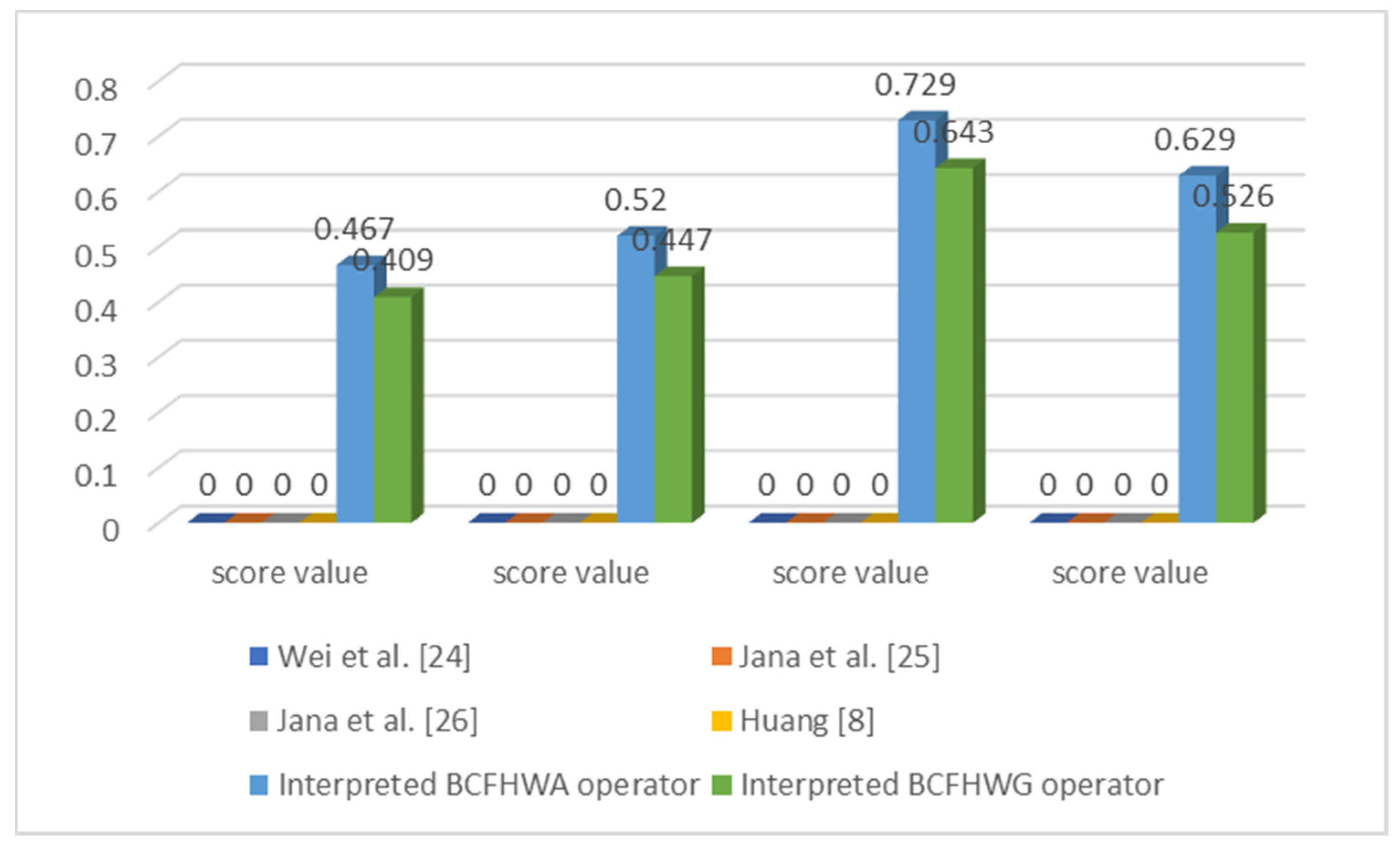From this, we observe that the work of Huang [8] is also unable to solve the MADM aspects involving the data in the environment of BCFSs. Only the interpreted work can solve such type of MADM cases. This shows that our approach is superior to the existing methods. BCFS amplifies the existing methods: when the imaginary part equals zero in both PD and ND, it transforms into BFSs, and if the imaginary part equals zero in PD and the ND part is neglected, its converts into FSs. The score values and ranking results of the interpreted and existing methods are given in

Table 2. Score values and ranking results of interpreted and existing work.

Methods	Score Values	Ranking
Wei et al. [24]	Failed	Failed
Jana et al. [25]	Failed	Failed
Jana et al. [26]	Failed	Failed
Huang [8]	Failed	Failed
Interpreted BCFHWA operator	${\mathcal{S}}_B\left({\mathfrak{x}}_1\right)=0.467$$, {\mathcal{S}}_B\left({\mathfrak{x}}_2\right)=0.52$$, {\mathcal{S}}_B\left({\mathfrak{x}}_3\right)=0.729$$, {\mathcal{S}}_B\left({\mathfrak{x}}_4\right)=0.629$	${\mathfrak{A}}_3\succ {\mathfrak{A}}_4\succ {\mathfrak{A}}_2\succ {\mathfrak{A}}_1$
Interpreted BCFHWG operator	${\mathcal{S}}_B\left({\mathfrak{x}}_1\right)=0.409$$, {\mathcal{S}}_B\left({\mathfrak{x}}_2\right)=0.447$$, {\mathcal{S}}_B\left({\mathfrak{x}}_3\right)=0.643$$, {\mathcal{S}}_B\left({\mathfrak{x}}_4\right)=0.526$	${\mathfrak{A}}_3\succ {\mathfrak{A}}_4\succ {\mathfrak{A}}_2\succ {\mathfrak{A}}_1$

. Figure 1 provides a graphic of the score values of existing and interpreted methods.

8. Conclusions

In this manuscript, we established various operations, the score function, and the accuracy function for BCFS. Furthermore, inspired by Hamacher operations, we interpreted BCFHWA operator, BCFHOWA operator, BCFHHA operator, BCFHWG operator, BCFHOWG operator, and BCFHHG operator. We described the features and the particular cases of the above operators such as BCFWA operator, BCFOWA operator, BCFHA operator, BCFWG operator, BCFOWG operator, and BCFHG operator by taking the parameter equal to 1. By taking the parameter equal to 2, we obtained BCFEWA operator, BCFEOWA operator, BCFEHA operator, BCFEWG operator, BCFEOWG operator, and BCFEHG operator. Subsequently, we used these operators to generate methods to resolve the bipolar complex fuzzy MADM issues. In order to authenticate the interpreted methods, we provided a numerical example for a company that has recruited the best employee for the position of assistant director.

Finally, in order to show the effectiveness and practicality of our approach, we compared our results with the existing operators.

The Hamacher operators based on BCFS generalize Hamacher operators for FS, BFS, and CFS. By obtaining the unreal part equal to zero in both PD and ND, we found Hamacher operators for the data in the structure of BFS; by neglecting the ND, we acquired Hamacher operators for CFS; and by obtaining the unreal part zero in PD and neglecting the ND, we acquired Hamacher operators for FS. However, our proposed approach presents some limitations, since the invented operators cannot manage the information in the structure of bipolar complex intuitionistic FS, bipolar complex fuzzy soft set, etc.

In the future, we shall use our operators and functions in different domains, such as complex fuzzy N-soft sets [47], complex hesitant FS [48], complex dual hesitant FSs [49,50], picture fuzzy N-soft sets [51], complex spherical FS [52], complex Pythagorean FS [53], generalized intuitionistic fuzzy hypergroupoid [54], and decision-making [55,56].

References

1. Zadeh, L.A. Fuzzy sets. Inf. Control. 1965, 8, 338–353. [Google Scholar] [CrossRef] [Green Version]
2. Mardani, A.; Nilashi, M.; Zavadskas, E.K.; Awang, S.R.; Zare, H.; Jamal, N.M. Decision Making Methods Based on Fuzzy Aggregation Operators: Three Decades Review from 1986 to 2017. Int. J. Inf. Technol. Decis. Mak. 2018, 17, 391–466. [Google Scholar] [CrossRef]
3. Merigó, J.M.; Casanovas, M. Fuzzy generalized hybrid aggregation operators and its application in fuzzy decision making. Int. J. Fuzzy System. 2010, 12, 15–24. [Google Scholar]
4. Atanassov, K. Intuitionistic fuzzy sets. Fuzzy Sets Syst. 1986, 20, 87–96. [Google Scholar] [CrossRef]
5. Xu, Z. Intuitionistic Fuzzy Aggregation Operators. IEEE Trans. Fuzzy Syst. 2007, 15, 1179–1187. [Google Scholar] [CrossRef]
6. Rahman, K.; Ayub, S.; Abdullah, S. Generalized intuitionistic fuzzy aggregation operators based on confidence levels for group decision making. Granul. Comput. 2020, 6, 867–886. [Google Scholar] [CrossRef]
7. Verma, R.; Merigó, J.M. Multiple attribute group decision making based on 2-dimension linguistic intuitionistic fuzzy aggregation operators. Soft Comput. 2020, 24, 17377–17400. [Google Scholar] [CrossRef]
8. Huang, J.-Y. Intuitionistic fuzzy Hamacher aggregation operators and their application to multiple attribute decision making. J. Intell. Fuzzy Syst. 2014, 27, 505–513. [Google Scholar] [CrossRef]
9. Garg, H. Intuitionistic Fuzzy Hamacher Aggregation Operators with Entropy Weight and Their Applications to Multi-criteria Decision-Making Problems. Iran. J. Sci. Technol. Trans. Electr. Eng. 2019, 43, 597–613. [Google Scholar] [CrossRef]
10. Zhang, W.R. Bipolar fuzzy sets and relations: A computational framework for cognitive modeling and multiagent decision analysis. In NAFIPS/IFIS/NASA’94, Proceedings of the First International Joint Conference of The North American Fuzzy Information Processing Society Biannual Conference. The Industrial Fuzzy Control and Intellig, San Antonio, TX, USA, 18–21 December 1994; IEE: Piscataway, NJ, USA, 1994; pp. 305–309. [Google Scholar]
11. Zhang, W.R. (Yin)(Yang) bipolar fuzzy sets. In Proceedings of the IEEE International Conference on Fuzzy Systems Proceedings. IEEE World Congress on Computational Intelligence (Cat. No. 98CH36228), Anchorage, AK, USA, 4–9 May 1998; Volume 1, pp. 835–840. [Google Scholar]
12. Lee, K.-M. Comparison of Interval-valued fuzzy sets, Intuitionistic fuzzy sets, and bipolar-valued fuzzy sets. J. Korean Inst. Intell. Syst. 2004, 14, 125–129. [Google Scholar] [CrossRef] [Green Version]
13. Zhang, W.-R.; Zhang, L. YinYang bipolar logic and bipolar fuzzy logic. Inf. Sci. 2004, 165, 265–287. [Google Scholar] [CrossRef]
14. Han, Y.; Shi, P.; Chen, S. Bipolar-Valued Rough Fuzzy Set and Its Applications to the Decision Information System. IEEE Trans. Fuzzy Syst. 2015, 23, 2358–2370. [Google Scholar] [CrossRef]
15. Yang, H.L.; Li, S.G.; Yang, W.H.; Lu, Y. Notes on “Bipolar fuzzy graphs”. Inf. Sci. 2013, 242, 113–121. [Google Scholar] [CrossRef]
16. Akram, M. Bipolar fuzzy graphs. Inf. Sci. 2011, 181, 5548–5564. [Google Scholar] [CrossRef]
17. Zhang, W.-R. Bipolar Quantum Logic Gates and Quantum Cellular Combinatorics—A Logical Extension to Quantum Entanglement. J. Quantum Inf. Sci. 2013, 3, 93–105. [Google Scholar] [CrossRef] [Green Version]
18. Zhang, W.-R.; Peace, K.E. Causality Is Logically Definable—Toward an Equilibrium-Based Computing Paradigm of Quantum Agent and Quantum Intelligence (QAQI) (Survey and Research). J. Quantum Inf. Sci. 2014, 4, 227–268. [Google Scholar] [CrossRef] [Green Version]
19. Zhang, W.-R.; Zhang, J.H.; Shi, Y.; Chen, S.-S. BIPOLAR LINEAR ALGEBRA AND YINYANG-N-ELEMENT CELLULAR NETWORKS FOR EQUILIBRIUM-BASED BIOSYSTEM SIMULATION AND REGULATION. J. Biol. Syst. 2009, 17, 547–576. [Google Scholar] [CrossRef]
20. Lu, M.; Busemeyer, J.R. Do traditional Chinese theories of Yi Jing (’Yin-Yang’ and Chinese medicine go beyond Western concepts of mind and matter. Mind Matter 2014, 12, 37–59. [Google Scholar]
21. Zhang, W.-R. G-CPT Symmetry of Quantum Emergence and Submergence—An Information Conservational Multiagent Cellular Automata Unification of CPT Symmetry and CP Violation for Equilibrium-Based Many-World Causal Analysis of Quantum Coherence and Decoherence. J. Quantum Inf. Sci. 2016, 6, 62–97. [Google Scholar] [CrossRef] [Green Version]
22. Zhang, W.R. YinYang bipolar relativity: A unifying theory of nature, agents and causality with applications in quantum computing, cognitive informatics and life sciences. IGI Global. 2011. [Google Scholar] [CrossRef]
23. Gul, Z. Some Bipolar Fuzzy Aggregations Operators and Their Applications in Multicriteria Group Decision Making. M. Ph.D. Thesis, Hazara University, Mansehra, Pakistan, 2015. [Google Scholar]
24. Wei, G.; Alsaadi, F.E.; Hayat, T.; Alsaedi, A. Bipolar Fuzzy Hamacher Aggregation Operators in Multiple Attribute Decision Making. J. Intell. Fuzzy Syst. 2018, 20, 1–12. [Google Scholar] [CrossRef]
25. Jana, C.; Pal, M.; Wang, J.-Q. Bipolar fuzzy Dombi aggregation operators and its application in multiple-attribute decision-making process. J. Ambient. Intell. Humaniz. Comput. 2019, 10, 3533–3549. [Google Scholar] [CrossRef]
26. Jana, C.; Pal, M.; Wang, J.-Q. Bipolar fuzzy Dombi prioritized aggregation operators in multiple attribute decision making. Soft Comput. 2020, 24, 3631–3646. [Google Scholar] [CrossRef]
27. Riaz, M.; Tehrim, S.T. A robust extension of VIKOR method for bipolar fuzzy sets using connection numbers of SPA theory based metric spaces. Artif. Intell. Rev. 2021, 54, 561–591. [Google Scholar] [CrossRef]
28. Sarwar, M.; Akram, M.; Zafar, F. Decision Making Approach Based on Competition Graphs and Extended TOPSIS Method under Bipolar Fuzzy Environment. Math. Comput. Appl. 2018, 23, 68. [Google Scholar] [CrossRef] [Green Version]
29. Mahmood, T. A Novel Approach towards Bipolar Soft Sets and Their Applications. J. Math. 2020, 2020, 1–11. [Google Scholar] [CrossRef]
30. Abdullah, S.; Aslam, M.; Ullah, K. Bipolar fuzzy soft sets and its applications in decision making problem. J. Intell. Fuzzy Syst. 2014, 27, 729–742. [Google Scholar] [CrossRef] [Green Version]
31. Ramot, D.; Milo, R.; Friedman, M.; Kandel, A. Complex fuzzy sets. IEEE Trans. Fuzzy Syst. 2002, 10, 171–186. [Google Scholar] [CrossRef]
32. Luqman, A.; Akram, M.; Al-Kenani, A.N.; Alcantud, J.C.R. A Study on Hypergraph Representations of Complex Fuzzy Information. Symmetry 2019, 11, 1381. [Google Scholar] [CrossRef] [Green Version]
33. Tamir, D.E.; Jin, L.; Kandel, A. A new interpretation of complex membership grade. Int. J. Intell. Syst. 2011, 26, 285–312. [Google Scholar] [CrossRef]
34. Yazdanbakhsh, O.; Dick, S. A systematic review of complex fuzzy sets and logic. Fuzzy Sets Syst. 2018, 338, 1–22. [Google Scholar] [CrossRef]
35. Tamir, D.E.; Rishe, N.D.; Kandel, A. Complex fuzzy sets and complex fuzzy logic an overview of theory and applications. In Fifty Years of Fuzzy Logic and Its Applications; Studies in Fuzziness and Soft Computing; Springer: Cham, Switzerland, 2015; Volume 326, pp. 661–681. [Google Scholar]
36. Dagher, I. Complex fuzzy c-means algorithm. Artif. Intell. Rev. 2012, 38, 25–39. [Google Scholar] [CrossRef]
37. Bi, L.; Dai, S.; Hu, B. Complex Fuzzy Geometric Aggregation Operators. Symmetry 2018, 10, 251. [Google Scholar] [CrossRef] [Green Version]
38. Hu, B.; Bi, L.; Dai, S. Complex Fuzzy Power Aggregation Operators. Math. Probl. Eng. 2019, 2019, 1–7. [Google Scholar] [CrossRef]
39. Bi, L.; Dai, S.; Hu, B.; Li, S. Complex fuzzy arithmetic aggregation operators. J. Intell. Fuzzy Syst. 2019, 36, 2765–2771. [Google Scholar] [CrossRef]
40. Garg, H.; Rani, D. Novel aggregation operators and ranking method for complex intuitionistic fuzzy sets and their applications to decision-making process. Artif. Intell. Rev. 2019, 5, 1–26. [Google Scholar] [CrossRef]
41. Mahmood, T.; Ur Rehman, U.; Ali, Z.; Mahmood, T. Hybrid vector similarity measures based on complex hesitant fuzzy sets and their applications to pattern recognition and medical diagnosis. J. Intell. Fuzzy Syst. 2021, 1–22. [Google Scholar] [CrossRef]
42. Behera, D.; Chakraverty, S. A new method for solving real and complex fuzzy systems of linear equations. Comput. Math. Model. 2012, 23, 507–518. [Google Scholar] [CrossRef]
43. Ur Rehman, U.; Mahmood, T.; Ali, Z.; Panityakul, T. A Novel Approach of Complex Dual Hesitant Fuzzy Sets and Their Applications in Pattern Recognition and Medical Diagnosis. J. Math. 2021, 2021, 1–31. [Google Scholar] [CrossRef]
44. Ma, X.; Zhan, J.; Khan, M.; Zeeshan, M.; Anis, S.; Awan, A.S. Complex fuzzy sets with applications in signals. Comput. Appl. Math. 2019, 38, 1–34. [Google Scholar] [CrossRef]
45. Mahmood, T.; Ur Rehman, U. A novel approach towards bipolar complex fuzzy sets and their applications in generalized similarity measures. Int. J. Intell. Syst. 2021. [Google Scholar] [CrossRef]
46. Hamacher, H. Über logische Verknüpfungen unscharfer Aussagen und deren zugehörige Bewertungsfunktionen. In Progress in Cybernetics and Systems Research, III; Trappl, R., Klir, G.J., Ricciardi, L., Eds.; RWT: Aachen, Germany, 1975; pp. 276–288. [Google Scholar]
47. Mahmood, T.; Ur Rehman, U.; Ali, Z. A novel complex fuzzy N-soft sets and their decision-making algorithm. Complex Intell. Syst. 2021, 7, 2255–2280. [Google Scholar] [CrossRef]
48. Mahmood, T.; Ur Rehman, U.; Ali, Z.; Chinram, R. Jaccard and Dice Similarity Measures Based on Novel Complex Dual Hesitant Fuzzy Sets and Their Applications. Math. Probl. Eng. 2020, 2020, 1–25. [Google Scholar] [CrossRef]
49. Chinram, R.; Mahmood, T.; Ur Rehman, U.; Ali, Z.; Iampan, A. Some Novel Cosine Similarity Measures Based on Complex Hesitant Fuzzy Sets and Their Applications. J. Math. 2021, 2021, 6690728. [Google Scholar] [CrossRef]
50. Mahmood, T.; Ur Rehman, U.; Ali, Z. Exponential and non-Exponential Based Generalized Similarity Measures for Complex Hesitant Fuzzy Sets with Applications. Fuzzy Inf. Eng. 2020, 12, 38–70. [Google Scholar] [CrossRef]
51. Ur Rehman, U.; Mahmood, T. Picture Fuzzy N-Soft Sets and Their Applications in Decision-Making Problems. Fuzzy Inf. Eng. 2021, 13, 335–367. [Google Scholar] [CrossRef]
52. Akram, M.; Khan, A.; Alcantud, J.C.R.; Santos-García, G. A hybrid decision-making framework under complex spherical fuzzy prioritized weighted aggregation operators. Expert Syst. 2021, 6, e12712. [Google Scholar] [CrossRef]
53. Ma, X.; Akram, M.; Zahid, K.; Alcantud, J.C.R. Group decision-making framework using complex Pythagorean fuzzy information. Neural Comput. Appl. 2021, 33, 2085–2105. [Google Scholar] [CrossRef]
54. Konwar, N.; Davvaz, B.; Debnath, P. Results on generalized intuitionistic fuzzy hypergroupoids. J. Intell. Fuzzy Syst. 2019, 36, 2571–2580. [Google Scholar] [CrossRef]
55. Gao, Y.; Zhang, Z. Consensus reaching with non-cooperative behavior management for personalized individual semantics-based social network group decision making. J. Oper. Res. Soc. 2021, 1–18. [Google Scholar] [CrossRef]
56. Zhang, Z.; Li, Z.; Gao, Y. Consensus reaching for group decision making with multi-granular unbalanced linguistic information: A bounded confidence and minimum adjustment-based approach. Inf. Fusion 2021, 74, 96–110. [Google Scholar] [CrossRef]
Figure 1. The graphical depiction of the score values of existing and interpreted work.
Mathematics 10 00023 g001