Abstract
This study evaluates the genetic diversity of different meagre broodstocks sampled in Greece. A multiplex of twelve microsatellite markers was used to genotype 946 fish from eleven stocks and batches used for broodstock selection, and the genetic data was used to calculate genetic population parameters as well as to investigate the genetic differentiation between stocks. The results from a relatedness analysis were used as the guiding lines for a fine-tuned and overall evaluation of the genetic distance between stocks, and the choice of candidate breeders from some of them. The approach implemented in this study uses well-established population genetics methods to evaluate the selection of breeder candidates in aquaculture commercial conditions utilizing a descriptive genetic data set based on microsatellite analyses, and to outline an efficient methodology for establishing the basis of new breeding schemes.
1. Introduction
Over 440 species of fish, invertebrates, and plants are farmed all over the world (www.fao.org/fishery/statistics/global-aquaculture-production/en, accessed on 1 December 2021. Genetic diversity is at the base of a variety of shapes, sizes, behavior, and colors that make aquatic species valuable and interesting. It also allows species to adapt to new farming systems, habitats, and environmental conditions. Higher genetic diversity implies more varieties and strains of organisms, which leads to greater adaptation possibilities in the challenging times of climate change and overfishing [1,2,3]. Marine fish species exhibit naturally high levels of genetic diversity, which is putatively the main driver of the rapid rate of genetic improvement, compared to plants or livestock [4,5,6,7]. Highly fecund species or r-strategists, like fish, exhibit higher polymorphism than species which produce low numbers of eggs and/or offspring of bigger body size, also termed K-strategists, with the propagule size (the size of the stage that leaves its parents and disperses, egg or juvenile) being highly predictive of a species’ genetic diversity [8,9]. Moreover, high genetic diversity provides a good foundation for genetic improvement, by making the broadening of the spectrum for selection objectives possible as well as utilizing the genetic diversity of the respective traits in the base population. The success of genetic improvement is attributed partly to capturing the broad range of genetic diversity at the start of a breeding program [10], while other factors are also in play. Genetic drift and inbreeding are the main causes of genetic diversity loss in closed populations, and increase when the effective population size is low [11]. Due to the rise in homozygosity, recessive deleterious alleles may also accumulate, resulting most of the times in a fitness depression which amplifies over time [12]. On the other hand, an increase in fitness is expected in populations that are genetically diverse, and this can lead to a high effective population size. A population with a high effective population size, as far as randomly selected neutral loci are concerned, is more likely to contain genes with variants affecting traits, thus increasing the performance of the stock and its ability to adapt to new farming systems and environments. However, genetic purging is evident in wild populations of fish species with low population sizes or low genetic diversity estimates, as well as for populations that have persisted in low sizes and in an environmental niche since their formation [13]. Moreover, purging in wild populations of low size may have assuaged the effects deleterious alleles have on fitness, thus preventing a decline in fitness [14], considering that the population sizes are not extremely low, i.e., below critical thresholds [15], making these populations highly specialized and at the same time vulnerable to new selective pressures. Studies of broodstock genetic diversity utilizing DNA markers are a common tool for conservation planning or breeding programs, with the Chinese sucker Myxocyprinus asiaticus [16], the European huchen Hucho hucho [17], tilapias [18], the barramundi Lates calcarifer [19], the European sea bass Dicentrarchus labrax, and the gilthead sea bream Sparus aurata [20,21] being some of the most recent ones. Polymorphic DNA markers have expanded the frontiers of research providing new insights into the genetic structure of fish populations [22,23,24], the intensity of natural and sexual selection, and the levels of inbreeding and disassortative mating success of alternative reproductive strategies [25]. The characteristics that microsatellites demonstrate make them very useful as genetic markers for studies of stock identification and population differentiation [26,27], such as the present one.
The meagre Argyrosomus regius (Asso, 1801) is a member of the Sciaenidae family, reaching a weight of 50 kg on average and over 180 cm in total length (FishBase.org). It is a semi-pelagic species found in the coastal areas of Senegal to the Bay of Biscay, in the eastern Atlantic Ocean, across the Mediterranean Sea, the Gulf of Suez, and the Black Sea. The species demonstrates a good potential for large scale aquaculture due to its high feed conversion ratio (FCR) and fast growth rate [28], and has emerged as a promising species for Mediterranean aquaculture [29]. The aquaculture production of meagre in the Mediterranean area exceeded 41 thousand tonnes in 2019, showing a growth of 10.5% compared to the previous year, while an additional growth of 2.8% is expected actually (APROMAR, 2020 http://apromar.es/, accessed on 1 December 2021), with Egypt producing the greatest part (approx. 75%) of this production, followed by Spain (9%), Turkey (6%), and Greece (4%). Despite some attractive attributes of meagre, such as the large size, good processing yield, low fat content, excellent taste, and firm texture [30], there are few major drawbacks identified, such as the limited genetic variation of the available broodstocks, variable growth rates, and the wide occurrence of systemic granulomatosis which constitute bottlenecks to the expansion of the industry [31].
The objectives of the current study were to assess the genetic diversity in different meagre breeders and offspring stocks based on microsatellite markers and then use this information to illustrate their putative relatedness, inbreeding, and population structure. The results outline the importance of implementing cost-effective population genetics analytical tools, for the genetic evaluation of breeding stocks as the starting point for the future design and fine-tuning of breeding programs.
2. Materials and Methods
2.1. Sampling
In September 2017, 302 meagre samples were collected from 8 breeder stocks (A–H) aged more than 6 years old that were purchased from commercial companies, except stock G, which was composed of wild fish. The last three stocks (I–K) were sampled in June 2020 and consisted of 643 offspring (younger than 4 years old) of the stocks A–H (www.diversifyfish.eu/uploads/1/4/2/0/14206280/diversify_featured_article_aes_42_sept_2017.pdf, accessed on 10 April 2018) [32] (Table S1).
2.2. DNA Techniques/PCR and Microsatellite Genotyping
DNA was extracted from all 946 samples using standard protocols [33] and DNA quality and quantity was evaluated using a NanoDrop ND 1000 spectrophotometer (Thermo Fisher Scientific; www.thermofisher.com, accessed on 10 April 2018). One multiplex PCR designed with 12 microsatellite loci [34] was developed for sciaenid species phylogenetically close to meagre and was optimized [35] using the Qiagen multiplex PCR kit. PCR reactions were performed in a 10 μL reaction mix with a concentration of 10 pmol/L for each primer and 5 ng/μL template DNA. The thermal profile included a pre-denaturation step at 95 °C for 15 min followed by 30 cycles of denaturation–annealing–extension at 94 °C for 30 s, 57 °C for 1.3 min, and 72 °C for 1 min and one final elongation step of 60 °C for 30 min. Amplicons were resolved by capillary electrophoresis on an ABI 3730 sequencer (Applied Biosystems, Foster City, CA, USA) using a LIZ500 size standard marker. The fragment size analysis software STRand (http://www.vgl.ucdavis.edu/informatics/STRand, accessed on 10 April 2018) was used for allele scoring.
2.3. Population Genetics Analysis
2.3.1. Genetic Variability and Departure from Hardy–Weinberg Equilibrium
The mean number of alleles per locus (Na), the observed (Hobs) and unbiased expected (He) heterozygosity [36], and Shannon’s diversity index [37] were computed for each stock and locus using GENETIX 4.05.2 [38] and GenAlEx v. 6.5 [39]. The departure of genotypic frequencies from the expectations of Hardy–Weinberg equilibrium (HWE) was estimated by the inbreeding coefficient or Wright’s fixation index (FIS) using Weir and Cockerham’s [40] f-estimator. The significance of the FIS values (i.e., consistency with the null hypothesis on HWE) was estimated after 10,000 random allelic permutations using a simple Bonferroni procedure to correct for multiple testing and avoid type-1 errors [41]. The presence of null alleles or other genotyping errors were estimated for all loci and collection sites using the Micro-Checker program version 2.2.3 [42].
2.3.2. Population Structure
Structure 2.3.2 [43] was used to infer the most likely population structure based on microsatellite data for the 11 meagre stocks. The population structure was estimated with a non-admixture model, without a priori population information, using a burn-in period of 250,000 and 1,000,000 subsequent MCMC repeats for each K value between 1 and 11 for 6 iterations. Then, Evanno’s ΔK method [44] was used as an aid to define the most informative partition by calculating the variation of the rate of likelihood between K and K + 1. These values correspond to local maxima of the curve ΔK function of K. The best K value was automatically calculated by the online program Structure Harvester (http://taylor0.biology.ucla.edu/structureHarvester/, accessed on 10 August 2019).
Furthermore, the stocks were re-assessed for population structuring using a discriminant analysis of principal components (DAPC) with the “adegenet” package [45] in R. This analysis was performed ab initio using just the raw data. DAPC analysis is divided into a PCA (principal component analysis) which is performed first and a second DA analysis (discriminant component analysis). PCA transforms the data and DA identifies the number of genetic groups that best fit the data structure by using a linear transformation searching for the maximum allelic variance between groups and the minimum allelic variance inside groups. The assigned IDs from DAPC and Structure were juxtaposed and combined in order to identify the common and different IDs as well as the composition of these differences. Additional PCA analyses were carried out using the adegenet package to examine the genetic grouping of the founding stocks using only the principal components and the putative overestimation of the DAPC grouping results.
2.4. Relatedness Analysis
Coancestry (V1.0.1.9) software implements seven methods for the estimation of the relatedness between individuals and four methods for the estimation of individual inbreeding coefficients using individual genotypes [46]. Initially, a preliminary run was performed using all 7 methods, and the summary statistics were used as the information upon which the methods with less variance and the highest correlation were tested with a simulation to evaluate their fitness to the data. The simulation was performed using the R package “related” [47], and was based on all given genotypes, from which 400 pairs of relationships were simulated for the 4 chosen relationship types (1600 in total): parent–offspring (PO), unrelated (UR), full-sibs (FS), and half-sibs (HS), respectively. The two maximum likelihood methods were chosen based on the summary statistics of the preliminary analysis (DyadML and TrioML), along with a non-maximum likelihood method [46]. Lastly, a linear regression between the simulation estimates and the summary statistics estimates for each method was performed to evaluate the fitness of the chosen simulation depth in relation to the whole dataset.
3. Results and Discussion
Population Genetics Indices
Micro-Checker results showed no evidence for scoring alleles due to stuttering, neither for large allele dropout nor the presence of null alleles. Linkage disequilibrium (LD) was estimated with the r2 method [48] and resulted in low estimates of LD in each stock; stocks D and E had the highest estimates, in the range of 22% and 29% of the theoretical (LD) maximum, respectively, while the rest of the stocks showed estimates below 0.1, ranging from 2% to 9% of the theoretical maximum. The slight LD observed in stock D might have been due to the low number (10) of individuals, while for stock E it may have been due to the slightly higher inbreeding estimates with respect to the rest of the stocks, shown also by its lower gene diversity and overall heterozygosity values. Heterozygosity values for each stock and for all microsatellite loci (Table 1) were generally low, with an average Hobs = 0.56, ranging from 0.40 in stock H to 0.83 in G. The number of alleles per locus was also generally low (average of 3.58, ranging from 2.5 to 5.0, see Table S1).

Table 1.
Heterozygosity values for 11 meagre stocks analysed with 12 microsatellite loci. The first column shows the microsatellite locus and columns 2–12 the corresponding heterozygosity values for each stock. The last two rows show the expected (He) and observed (Hobs) heterozygosity values for each stock. (In bold: the highest and lowest observed heterozygosity between the stocks.) The number of fish per stock is depicted in the first row.
Furthermore, the pattern of expected heterozygosity was not the same across stocks. The alleles that were shared by half or a quarter of the stocks and the unique alleles of each stock were differentiated, and this might be partly due to sample size differences between stocks, and thus a bias in allele sampling; e.g., in stock F there were just 6 samples, and in stock K there were 491. Likewise, stock H showed a reduced expected heterozygosity when using the Weir estimator for gene diversity or heterozygosity calculation (expected and observed). The observed and expected heterozygosity of the stocks did not change with the use of different methods, with stock G showing the largest and H the lowest (Figure 1).

Figure 1.
Heterozygosity pattern across stocks. Na: number of different alleles, Na (Freq ≥ 5%): number of different alleles with a frequency ≥5%, Ne: number of effective alleles = 1/(Sum pi2), I: Shannon’s information index = −1 × Sum (pi × Ln (pi)), No. Private Alleles: number of alleles unique to a single population, No. LComm Alleles (≤25%): number of locally common alleles (Freq. ≥ 5%) found in 25% or fewer populations, No. LComm Alleles (≤50%): number of locally common alleles (Freq. ≥ 5%) found in 50% or fewer populations, He: expected heterozygosity = 1 − Sum pi2.
The FIS index allows for understanding the evolutionary forces acting on populations. An excess or lack of heterozygosity in a population varies depending on the mating system, and whether and to what extent heterozygosity provides a selection advantage [49], with the mating system’s “genetic reflection” in the data being influenced by artificial (Wahlund effect, null alleles, inadequate allele sampling, insufficient or weak allelic dominance) or biological reasons (inbreeding, homogamy). Negative FIS values in a panmictic population, with a sample size considered representative, indicate an increased degree of mating between individuals less related to each other, while positive values indicate the opposite. The first eight stocks (A–H) consisted of breeders, so it makes sense to observe an increase in heterozygosity outside the statistically significant limits of the HW equilibrium, which were estimated from −0.11037 to −0.01097. In addition, D and F breeder stocks had the smallest numbers of fish with 6 and 10 individuals, respectively. This fact means these stocks are not very valuable in estimating the relatedness, inbreeding, and other population genetic parameters. Stock K, which was the largest, comprising 491 offspring, seemed to fall within the statistically significant limits for the majority of genetic loci, while stocks I and J showed similar values with some loci showing a higher variability (Table 2).
Table 2.
Wright’s FIS parameter estimates in stocks. The first column lists the microsatellite loci and column 2 to column 12 list the corresponding estimate for each stock.
The genetic structure of the stocks showed five groups, according to Evanno’s criterion [44]. In Figure 2, we show the best assignment of all fish from the 11 stocks to 5 genetic groups or clusters. Each colored column represents the probability of each individual participating in one of the five groups starting from the first one in stock A to the last in stock K. Although the grouping is not obvious at a glance, up to stock J individuals are assigned mainly to groups 2, 3, and 5 while stock K is assigned almost exclusively to 1 and 4. Additionally, group 3 appears to be present in all stocks. While Structure has been reported to provide inaccurate estimates when a uniform alpha prior is used to infer ancestry between populations of highly unequal sizes [50], this applies to the admixture model analysis and can be corrected with the use of a variable alpha prior option. However, in non-admixture analysis, the unequal sample sizes do not influence the results.

Figure 2.
Illustration of the assignment of all meagre fish from the 11 stocks to the 5 genetic groups after using the software Structure. Each column shows the individual probability of assignment to a genetic cluster, and the ID of each individual was added in R language environment.
DAPC analysis showed that the genetic groups 3 and 4 had the largest genetic distance between them, with groups 1, 2, and 5 showing the smallest distance (Figure 3).

Figure 3.
Analysis of DAPC (distinguishing components and main components) to find the optimal genetic grouping of the 11 stocks. The relative contribution of each genetic group to the overall picture has been included in the axes based on the results of PCA and DA.
Each of the Structure clusters were juxtaposed with the DAPC clusters to find the corresponding ones (Figure 4); at the y axis, the clusters that had the best alignment with each other in terms of the highest number of individuals shared between them can be observed, and at the x axis the number of total individuals in each cluster comparison can be seen. The corresponding clusters in Structure and DAPC had a range in difference from 5% to 19%.

Figure 4.
Comparison of the genetic groups identified by Structure and DAPC methods. The y axis shows the correspondence of the groups and the x axis shows the number of fish assigned to them, while DAPC grouping is used as a reference.
For convenience, DAPC grouping will be used as the reference. The differences between the two methods are mainly found in two groups: 2 and 5. This is evident from the DAPC graph (Figure 3) as groups 2 and 5 appear at close genetic distances with some degree of overlap while 3 and 4 show higher genetic distances in comparison. In addition, in group 5, out of the 60 different assigned samples, 48 belong to the stock K.
The discriminant part of the DAPC analysis performs the clustering by maximizing the genetic distances between groups, based on one optimal number of clusters, while PCA uses just the most informative principal components for the transformation and grouping of the data. For this reason, we performed additional PCA analyses using just the principal components to investigate the grouping of the founding stocks and the convergence with the overall results. The offspring were clustered in DAPC groups 1 and 5; hence, by removing them from the grouping procedure, the remaining groups would presumably show a higher distinction. The genetic grouping of the founding stocks, excluding the offspring populations I to K, corresponded with the overall results obtained with Structure and DAPC for the 11 stocks. Stocks C and G showed increased genetic distance from the rest, and A, B, D, E, F, and H showed genetic proximity (Figure S1). In the analysis with all the stocks used, C and G are found predominantly in the more divergent DAPC clusters 4 and 3, respectively (Figure 3) and A, B, D, E, F, and H are mostly in DAPC cluster 2. Due to the fact that stock C showed the highest genetic distance to the rest of the stocks, it was removed to highlight the differences in DAPC cluster 2, with the inbreeding of the stocks being indirectly and partially reflected in the PCA (Figure S2). In Supplementary Figure S2, the grouping of A, B, and F is shown to be distinct from that of E, H, D, and G, as in the box plot of Figure 7. In this way, a higher resolution inside cluster 2 of DAPC was achieved. Moreover, stock G, as shown in the Structure output (Figure 2), shows genetic similarity to stocks A and B, having private alleles which are shared by stock A and B exclusively (data not shown). The observed similarities between A, B, and G, coupled with the low inbreeding estimates of stock G (Figure 7), point most probably to a putative transfer of individuals between the founding stocks and/or to gene flow events in the life history of the natural populations these stocks originated from.
The results of the simulation are depicted in Figure 5 in the form of a box plot comparing the performance for each type of relationship of the 1600 simulated pairs. Moreover, a correlation estimate was performed for DyadML, TrioML, and Wang estimator values from the simulation results versus the observed values that were produced by a preliminary analysis, the summary statistics of which are shown in Table S3. DyadML showed the highest correlation with 0.7332, following by TrioML with 0.7281 and Wang with 0.6998. The expected values were calculated based on the results obtained from the real data. The correlation of the simulated relatedness of each estimator with the actual relatedness results (of the same estimators) investigates a misrepresentation that can arise from the chosen simulation depth. Since the performance of the estimators was comparable in the simulated and real data, the chosen simulation depth was deemed representative of the dataset. Indeed, DyadML and TrioML showed the smallest variance in all types of relationships and were the estimators that best fit our data, while the Wang estimator showed more variance, resulting in lower confidence estimations. Lastly, the outliers present in the box plot in Figure 5 denote some relationship estimates of the simulated pairs with higher or lower values, and are reflective of a range of inbreeding and outbreeding of the simulated genotypes based on the initial data, while the number of these outliers is negligible compared to the number of the simulated pairs.
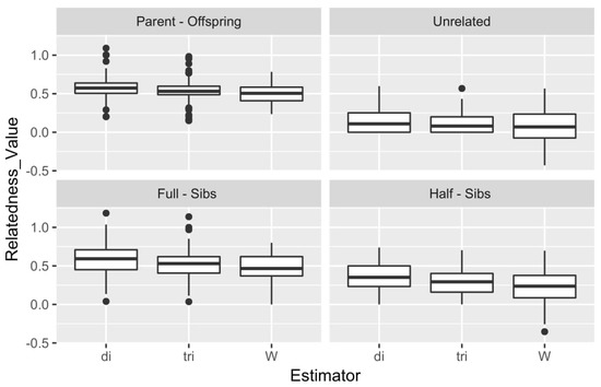
Figure 5.
Summary of the results for the 3 methods and the 4 types of simulated relationships. di: DyadML, tri: TrioML, W: Wang.
Although it is known that the stocks A to H were comprised of breeders, while stocks I to K were from mixed populations of offspring which will be used to select future broodstocks, we investigated the condition of inbreeding and the putative relatedness of all the stocks against each other. In this way, the actual integrity of the stocks is reflected, and the putative inbreeding of the initial natural populations of the breeder stocks is excluded. An “all versus all” relatedness analysis paves the way for a further verification of the population structure, and gives the additional possibility of re-adjusting the existing breeding scheme. The main objective was to dissect the relatedness of stocks I, J, and K with the rest, and obtain an evaluation of their range of inbreeding. Furthermore, from the relatedness analysis results, we compared the two estimators using as a grouping factor the relationships inside each stock (IS) as well as between stocks (OS), focusing more on the latter estimates. For this purpose, we removed the pairs of relatedness estimates that had 0 value, and hence were unrelated. Figure 6 expands on the issue, depicting two density plots for each estimator and a scatter plot with a correlation.
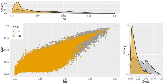
Figure 6.
Distribution of relationship estimates between stocks by DyadML and TrioML methods. The relationships shown in yellow (OS) refer to the relationships between different stocks, while those in grey (IS) refer to the relationships within the stocks. The value range corresponds for 0.125 to first cousins, 0.25 for half-siblings, and from 0.5 and more for full-sibs and parent–offspring. Zero values have been subtracted for the optimal display of the plots.
We notice that most of the estimated values concerning the pairwise relatedness estimations of individuals were between 0.1 and 0.4, with 0.25 being heavily present. Each value represents a putative relationship of the 447,458 pairs examined (946 * (946/2)). As a reminder, that values of 0.125 are for first cousins, 0.25 for half-sibs, and values greater than 0.5 for full-sibs and parent–offspring relationships. The correlation between the two estimators is to be expected, as stated before. In Figure 6, we see that most OS values (depicted with the yellow color between different stocks) are around 0.1, indicating a weak relatedness between the stocks. On the contrary, we observe as expected the IS values (inside each stock) being close to 0.5, indicating parent–offspring and/or full-sib relationships, which serves as an additional verification of the genetic differentiation between stocks and their viability as a basis of a new breeding scheme.
Since coancestry provides estimates of the inbreeding of each individual based on the relatedness estimates, we plotted the inbreeding estimates results from DyadML against the corresponding stocks and grouped them according to the common IDs (Structure and DAPC) using DAPC clusters from 1 to 5 as a reference. The results are depicted in the following box plot diagram in Figure 7.
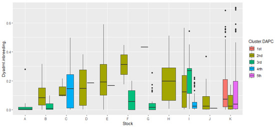
Figure 7.
Graphical representation of the correlation of inbreeding values in the 11 stocks as calculated by the DyadML method, with the 5 genetic groups from the common Structure–DAPC results, using the DAPC topology as a reference. On the y axis, the estimates of inbreeding are depicted, while on the x axis we show the stocks; the width of the box plot does not represent a parameter and is relative to the number of subdivisions inside a stock.
The less inbred stocks correlate with the 3rd and 4th cluster of DAPC, which is also evident in the DAPC depiction itself, with stock C showing some increased variance as well as high values in its inbreeding estimates in cluster 4. It is furthermore evident that the 2nd cluster of DAPC is the most genetically connected with the rest, and shows the highest inbreeding values while clearly specific stocks having in its composition: D, E, H, and J, which belong exclusively to it (cluster 2) and individuals from other stocks (B, C, I, and K) that are connected to it. Stock K seems to be divided, in terms of inbreeding and relatedness between clusters 1, 2, and 5, clusters that seem to have some genetic resemblance, which indicates that stock K founders may have originated from three different initial populations since stock K’s inbreeding estimates are relatively low. The outliers in offspring stocks K and I in Figure 7 are individuals that show higher inbreeding estimates than the inbreeding distribution range of these stocks, while proportionally they are more for stock I, showcasing a founder effect, since they are mostly connected with stock C and belong exclusively to cluster 4, while for stock K they are putative offspring originating from the mating of full-siblings or parent–offspring crosses. The 3rd DAPC cluster, containing fish from breeder stocks, showed small inbreeding estimates and higher genetic diversity overall, along with the 5th DAPC cluster which was comprised of offspring. In stock E, the 2nd cluster showed reduced genetic diversity while having higher inbreeding estimates, with the LD estimate being ~30% of the theoretical maximum. Moreover, the outliers in the breeder stock G can be putatively attributed to a transfer of fish from stocks A and B as was already pointed out, or gene flow events in the life histories of the natural populations of A, B, and G.
While meagre aquaculture has been ongoing for 30 years, few efforts have been made to address the requirement for rigorous tracking of genetic diversity, inbreeding, and genetic structure in commercial stocks. Numerous other species have lost genetic diversity as a consequence of the lack of a consistent genetic evaluation, which has already been well-documented [20,21,51,52,53,54,55]. In our study, the discrepancy between the effective allele size and the number of alleles in each stock showed that the genetic diversity is not shaped by low frequency alleles, but rather by the unequal frequencies of common alleles, with the low number of private alleles being indicative of that. Low frequency alleles, under neutrality or weak selection, are more prone to being wiped out by genetic drift and/or inbreeding, influencing epistatic interactions or removing adaptive potential. The number of private alleles as well as the heterozygosity estimates follow the pattern of inbreeding estimates, with stocks A, B, G, and I showing signatures of genetic differentiation from the rest of the stocks of breeders. Furthermore, the results highlight the rise of inbreeding as a result of ongoing introgression, which can further induce genetic drift and homozygosity after a few generations [21]. Although the wild populations where the meagre breeders originated from were not available for comparison purposes in this study, the choice of new breeders genetically more distant from the Atlantic–Western Mediterranean populations will enhance the genetic potential of the species as it introduces new genetic variation originating from different lineages [56]. We firmly believe that the findings of this study are important to the choice of new breeders for the sustainable development and growth of meagre aquaculture, and in addition the detailed methodology presented here can be part of the design for new selective breeding programs, as well as to adjust and evaluate ongoing ones.
4. Conclusions
We have successfully used microsatellite markers to infer genetic differentiation and population structure in commercial broodstocks as well as to study genetic drift, in-breeding and relatedness in offspring stocks. STRUCTURE and DAPC analyses of the microsatellite genotype data generally agree and identify five groups into the specimens studied. Furthermore, relatedness analysis indicates a weak relatedness between the stocks but a close one between fish into most of them which is of great importance to design and manage ongoing and future breeding programs.
Supplementary Materials
The following are available online at https://www.mdpi.com/article/10.3390/fishes6040078/s1, Figure S1: PCA analysis only for the eight breeder stocks A to H, Figure S2: PCA analysis using the breeder stocks A, B, D, E, F, G, H to highlight the resolution in cluster 2 from DAPC analysis of Figure 4, Table S1: Number of alleles for the twelve loci genotyped in meagre broodstocks, Table S2:. Statistical summary of the performance of Coancestry software methods in the exploratory analysis of the 11 stocks for method selection. The coefficient of linear correlation between all methods as well as their variance is given.
Author Contributions
Conceptualization, O.N., D.C. and C.S.T.; methodology, O.N. and C.S.T.; software, O.N. and C.S.T.; validation, D.C., C.B. and K.T.; formal analysis, O.N. and C.S.T.; investigation, O.N. and K.E.; resources, K.T. and L.P.; data curation, O.N. and C.S.T.; writing—original draft preparation, O.N. and C.S.T.; writing—review and editing, O.N., K.T., L.P., K.E., D.C., C.B. and C.S.T.; visualization, O.N.; supervision, C.S.T.; project administration, C.S.T.; funding acquisition, C.S.T. All authors have read and agreed to the published version of the manuscript.
Funding
Financial support was provided by the Hellenic General Secretariat for Research and Innovation (GSRI) through the project MeagreGEN (“Special Actions, AQUACULTURE”, Τ6ΥBP-00012) funded by EPAnEK (“Competitiveness, Entrepreneurship and Innovation, 2014–2020” operational programme). We also acknowledge the European Union’s Horizon 2020 research and innovation programme under grant agreement No. 652831 (AQUAEXCEL2020).
Institutional Review Board Statement
Sample providers complied with institutional, national, and international guidelines and regulations as well as the Nagoya protocol to obtain our fish clip samples. No ethics committee approval was necessary for the collection of fish clips. All fish treatments used for sampling were in accordance with the guidelines of the European Directive (2010/63/EU) on the protection of animals used for scientific purposes. In addition, A. regius is neither an endangered species nor a species at risk of extinction according to the IUCN (Red List category: Least Concern).
Conflicts of Interest
The authors declare that they have no competing interest.
References
- Milla, S.; Pasquet, A.; El Mohajer, L.; Fontaine, P. How domestication alters fish phenotypes. Rev. Aquac. 2021, 13, 388–405. [Google Scholar] [CrossRef]
- Elmer, K.R.; Kusche, H.; Lehtonen, T.K.; Meyer, A. Local variation and parallel evolution: Morphological and genetic diversity across a species complex of neotropical crater lake cichlid fishes. Philos. Trans. R. Soc. B Biol. Sci. 2010, 365, 1763–1782. [Google Scholar] [CrossRef]
- Carvalho, G.R. Evolutionary aspects of fish distribution: Genetic variability and adaptation. J. Fish Biol. 1993, 43, 53–73. [Google Scholar] [CrossRef]
- Gjedrem, T.; Robinson, N. Advances by Selective Breeding for Aquatic Species: A Review. Agric. Sci. 2014, 5, 1152–1158. [Google Scholar] [CrossRef]
- DeWoody, J.A.; Avise, J.C. Microsatellite variation in marine, freshwater and anadromous fishes compared with other animals. Fish Biol. 2005, 56, 461–473. [Google Scholar] [CrossRef]
- Baillie, S.M.; Muir, A.M.; Hansen, M.J.; Krueger, C.C.; Bentzen, P. Genetic and phenotypic variation along an ecological gradient in lake trout Salvelinus namaycush. BMC Evol. Biol. 2016, 16, 1–16. [Google Scholar] [CrossRef]
- Baillie, S.M.; Hemstock, R.R.; Muir, A.M.; Krueger, C.C.; Bentzen, P. Small-scale intraspecific patterns of adaptive immunogenetic polymorphisms and neutral variation in Lake Superior lake trout. Immunogenetics 2018, 70, 53–66. [Google Scholar] [CrossRef]
- Romiguier, J.; Gayral, P.; Ballenghien, M.; Bernard, A.; Cahais, V.; Chenuil, A.; Chiari, Y.; Dernat, R.; Duret, L.; Faivre, N.; et al. Comparative population genomics in animals uncovers the determinants of genetic diversity. Nature 2014, 515, 261–263. [Google Scholar] [CrossRef]
- Ellegren, H.; Galtier, N. Determinants of genetic diversity. Nat. Rev. Genet. 2016, 17, 422–433. [Google Scholar] [CrossRef]
- Gjedrem, T.; Gjøen, H.M.; Gjerde, B. Genetic origin of Norwegian farmed Atlantic salmon. Aquaculture 1991, 98, 41–50. [Google Scholar] [CrossRef]
- Frankham, R.; Ballou, S.E.J.D.; Briscoe, D.A.; Ballou, J.D. Introduction to Conservation Genetics; Cambridge University Press: Cambridge, UK, 2002. [Google Scholar]
- Wang, S.; Hard, J.J.; Utter, F. Salmonid inbreeding: A review. Rev. Fish Biol. Fish. 2002, 11, 301–319. [Google Scholar] [CrossRef]
- Yates, M.C.; Bowles, E.; Fraser, D.J. Small population size and low genomic diversity have no effect on fitness in experimental translocations of a wild fish. Proc. R. Soc. B 2019, 286, 20191989. [Google Scholar] [CrossRef]
- Danzmann, R.G.; Morgan, R.P., II; Jones, M.W.; Bernatchez, L.; Ihssen, P.E. A major sextet of mitochondrial DNA phylogenetic assemblages extant in eastern North American brook trout (Salvelinus fontinalis): Distribution and postglacial dispersal patterns. Can. J. Zool. 1998, 76, 1300–1318. [Google Scholar] [CrossRef]
- Jamieson, I.G.; Allendorf, F.W. How does the 50/500 rule apply to MVPs? Trends Ecol. Evol. 2012, 27, 578–584. [Google Scholar] [CrossRef]
- Liu, D.; Zhou, Y.; Yang, K.; Zhang, X.; Chen, Y.; Li, C.; Li, H.; Song, Z. Low genetic diversity in broodstocks of endangered Chinese sucker, Myxocyprinus asiaticus: Implications for artificial propagation and conservation. ZooKeys 2018, 792, 117–132. [Google Scholar] [CrossRef]
- Kucinski, M.; Fopp-Bayat, D.; Liszewski, T.; Svinger, V.W.; Lebeda, I.; Kolman, R. Genetic analysis of four European huchen (Hucho hucho Linnaeus, 1758) broodstocks from Poland, Germany, Slovakia, and Ukraine: Implication for conservation. J. Appl. Genet. 2015, 56, 469–480. [Google Scholar] [CrossRef]
- Montoya-López, A.F.; Tarazona-Morales, A.M.; Olivera-Angel, M.; Betancur-López, J.J. Genetic diversity of four broodstocks of tilapia (Oreochromis sp.) from Antioquia, Colombia. Rev. Colomb. Cienc. Pecu. 2019, 32, 201–213. [Google Scholar] [CrossRef]
- Loughnan, S.R.; Smith-Keune, C.; Jerry, D.R.; Beheregaray, L.B.; Robinson, N.A. Genetic diversity and relatedness estimates for captive barramundi (Lates calcarifer, B loch) broodstock informs efforts to form a base population for selective breeding. Aquac. Res. 2016, 47, 3570–3584. [Google Scholar] [CrossRef]
- Loukovitis, D.; Sarropoulou, E.; Vogiatzi, E.; Tsigenopoulos, C.S.; Kotoulas, G.; Magoulas, A.; Chatziplis, D. Genetic variation in farmed populations of the gilthead sea bream Sparus aurata in Greece using microsatellite DNA markers. Aquac. Res. 2012, 43, 239–246. [Google Scholar] [CrossRef]
- Loukovitis, D.; Ioannidi, B.; Chatziplis, D.; Kotoulas, G.; Magoulas, A.; Tsigenopoulos, C.S. Loss of genetic variation in Greek hatchery populations of the European sea bass (Dicentrarchus labrax L.) as revealed by microsatellite DNA analysis. Mediterr. Mar. Sci. 2015, 16, 197–200. [Google Scholar] [CrossRef]
- Hansen, M.M.; Kenchington, E.; Nielsen, E.E. Assigning individual fish to populations using microsatellite DNA markers. Fish Fish. 2001, 2, 93–112. [Google Scholar] [CrossRef]
- Chistiakov, D.A.; Hellemans, B.; Volckaert, F.A. Microsatellites and their genomic distribution, evolution, function and applications: A review with special reference to fish genetics. Aquaculture 2006, 255, 1–29. [Google Scholar] [CrossRef]
- Layton, K.K.; Dempson, B.; Snelgrove, P.V.; Duffy, S.J.; Messmer, A.M.; Paterson, I.G.; Bradbury, I.R. Resolving fine-scale population structure and fishery exploitation using sequenced microsatellites in a northern fish. Evol. Appl. 2020, 13, 1055–1068. [Google Scholar] [CrossRef]
- Ferguson, M.M.; Danzmann, R.G. Role of genetic markers in fisheries and aquaculture: Useful tools or stamp collecting? Can. J. Fish. Aquat. Sci. 1998, 55, 1553–1563. [Google Scholar] [CrossRef]
- Wright, T.F.; Johns, P.M.; Walters, J.R.; Lerner, A.P.; Swallow, J.G.; Wilkinson, G.S. Microsatellite variation among divergent populations of stalk-eyed flies, genus Cyrtodiopsis. Genet. Res. 2004, 84, 27–40. [Google Scholar] [CrossRef]
- Liu, Z.J.; Cordes, J.F. DNA marker technologies and their applications in aquaculture genetics. Aquaculture 2004, 238, 1–37. [Google Scholar] [CrossRef]
- Fountoulaki, E.; Grigorakis, K.; Kounna, C.; Rigos, G.; Papandroulakis, N.; Diakogeorgakis, J.; Kokou, F. Growth performance and product quality of meagre (Argyrosomus regius) fed diets of different protein/lipid levels at industrial scale. Ital. J. Anim. Sci. 2017, 16, 685–694. [Google Scholar] [CrossRef]
- Duncan, N.J.; Estévez, A.; Fernández-Palacios, H.; Gairin, I.; Hernández-Cruz, C.M.; Roo, J.; Vallés, R. Aquaculture production of meagre (Argyrosomus regius): Hatchery techniques, ongrowing and market. In Advances in Aquaculture Hatchery Technology; Woodhead Publishing: Sawston, UK, 2013; pp. 519–541. [Google Scholar]
- Monfort, M.C. Present market situation and prospects of meagre (Argyrosomus regius), as an emerging species in mediterranean aquaculture. In Studies and Reviews-General Fisheries Commission for the Mediterranean; Food and Agriculture Organization of the United Nations (FAO): Rome, Italy, 2010. [Google Scholar]
- Tsertou, M.I.; Smyrli, M.; Kokkari, C.; Antonopoulou, E.; Katharios, P. The aetiology of systemic granulomatosis in meagre (Argyrosomus regius): The “Nocardia” hypothesis. Aquac. Rep. 2018, 12, 5–11. [Google Scholar] [CrossRef]
- Exploring the Biological and Socio-Economic Potential of New/Emerging Candidate Fish Species for the Expansion of the European Aquaculture Industry. 2017. Available online: www.diversifyfish.eu/uploads/1/4/2/0/14206280/di-versify_featured_article_aes_42_sept_2017.pdf (accessed on 10 April 2019).
- Miller, S.A.; Dykes, D.D.; Polesky, H.F. A simple salting out procedure for extracting DNA from human nucleated cells. Nucleic Acids Res. 1988, 16, 1215. [Google Scholar] [CrossRef]
- Schuelke, M. An economic method for the fluorescent labeling of PCR fragments. Nat. Biotechnol. 2000, 18, 233–234. [Google Scholar] [CrossRef] [PubMed]
- Nousias, O.; Tsakogiannis, A.; Duncan, N.; Villa, J.; Tzokas, K.; Estevez, A.; Chatziplis, D.; Tsigenopoulos, C.S. Parentage assignment, estimates of heritability and genetic correlation for growth-related traits in meagre Argyrosomus regius. Aquaculture 2020, 518, 734663. [Google Scholar] [CrossRef]
- Nei, M. Estimation of average heterozygosity and genetic distance from a small number of individuals. Genetics 1978, 89, 583–590. [Google Scholar] [CrossRef]
- Shannon, C.E.; Weaver, W. The Mathematical Theory of Information; University of Illinois Press: Urbana, IL, USA, 1949; Volume 97. [Google Scholar]
- Belkhir, K. GENETIX 4.05, Logiciel Sous Windows TM Pour la Génétique des Populations. 2004. Available online: http://www.genetix.univ-montp2.fr/genetix/genetix.htm (accessed on 10 August 2019).
- Peakall, R.; Smouse, P.E. GenAlEx 6.5: Genetic analysis in Excel. Population genetic software for teaching and research. Bioinformatics 2012, 28, 2537–2539. [Google Scholar] [CrossRef] [PubMed]
- Weir, B.S.; Cockerham, C.C. Estimating F-statistics for the analysis of population structure. Evolution 1984, 38, 1358–1370. [Google Scholar]
- Rice, W.R. Analyzing tables of statistical tests. Evolution 1989, 43, 223–225. [Google Scholar] [CrossRef]
- Van Oosterhout, C.; Hutchinson, W.F.; Wills, D.P.; Shipley, P. MICRO-CHECKER: Software for identifying and correcting genotyping errors in microsatellite data. Mol. Ecol. Notes 2004, 4, 535–538. [Google Scholar] [CrossRef]
- Falush, D.; Stephens, M.; Pritchard, J.K. Inference of population structure using multilocus genotype data: Linked loci and correlated allele frequencies. Genetics 2003, 164, 1567–1587. [Google Scholar] [CrossRef]
- Evanno, G.; Regnaut, S.; Goudet, J. Detecting the number of clusters of individuals using the software STRUCTURE: A simulation study. Mol. Ecol. 2005, 14, 2611–2620. [Google Scholar] [CrossRef]
- Jombart, T. Adegenet: A R package for the multivariate analysis of genetic markers. Bioinformatics 2008, 24, 1403–1405. [Google Scholar] [CrossRef]
- Wang, J. COANCESTRY: A program for simulating, estimating and analysing relatedness and inbreeding coefficients. Mol. Ecol. Resour. 2011, 11, 141–145. [Google Scholar] [CrossRef]
- Pew, J.; Muir, P.H.; Wang, J.; Frasier, T.R. Related: An R package for analysing pairwise relatedness from codominant molecular markers. Mol. Ecol. Resour. 2015, 15, 557–561. [Google Scholar] [CrossRef]
- Hill, W.G.; Robertson, A. Linkage disequilibrium in finite populations. Theor. Appl. Genet. 1968, 38, 226–231. [Google Scholar] [CrossRef]
- Wright, S. The Theory of Gene Frequencies Evolution and the Genetics of Populations: A Treatise in Three Volumes; No. 576.58 W9301t Ej. 1 025186; The University of Chicago Press: Chicago, IL, USA, 1969. [Google Scholar]
- Wang, J. The computer program structure for assigning individuals to populations: Easy to use but easier to misuse. Mol. Ecol. Resour. 2017, 17, 981–990. [Google Scholar] [CrossRef] [PubMed]
- Evans, B.; Bartlett, J.; Sweijd, N.; Cook, P.; Elliott, N.G. Loss of genetic variation at microsatellite loci in hatchery produced abalone in Australia (Haliotis rubra) and South Africa (Haliotis midae). Aquaculture 2004, 233, 109–127. [Google Scholar] [CrossRef]
- Li, Q.; Park, C.; Endo, T.; Kijima, A. Loss of genetic variation at microsatellite loci in hatchery strains of the Pacific abalone (Haliotis discus hannai). Aquaculture 2004, 235, 207–222. [Google Scholar] [CrossRef]
- Alam, M.S.; Islam, M.S. Population genetic structure of Catla catla (Hamilton) revealed by microsatellite DNA markers. Aquaculture 2005, 246, 151–160. [Google Scholar] [CrossRef]
- Lundrigan, T.A.; Reist, J.D.; Ferguson, M.M. Microsatellite genetic variation within and among Arctic charr (Salvelinus alpinus) from aquaculture and natural populations in North America. Aquaculture 2005, 244, 63–75. [Google Scholar] [CrossRef]
- Li, Q.; Xu, K.; Yu, R. Genetic variation in Chinese hatchery populations of the Japanese scallop (Patinopecten yessoensis) inferred from microsatellite data. Aquaculture 2007, 269, 211–219. [Google Scholar] [CrossRef]
- Haffray, P.; Malha, R.; Sidi, M.O.T.; Prista, N.; Hassan, M.; Castelnaud, G.; Karahan-Nomm, B.; Gamsiz, K.; Sadek, S.; Bruant, J.S.; et al. Very high genetic fragmentation in a large marine fish, the meagre Argyrosomus regius (Sciaenidae, Perciformes): Impact of reproductive migration, oceanographic barriers and ecological factors. Aquat. Living Resour. 2012, 25, 173–183. [Google Scholar] [CrossRef]


Publisher’s Note: MDPI stays neutral with regard to jurisdictional claims in published maps and institutional affiliations. |
© 2021 by the authors. Licensee MDPI, Basel, Switzerland. This article is an open access article distributed under the terms and conditions of the Creative Commons Attribution (CC BY) license (https://creativecommons.org/licenses/by/4.0/).