
Impact of Demand Response on Reliability Enhancement in Distribution Networks

Abstract
:1. Introduction
1.1. Aim
1.2. Literature Review
1.3. Contributions
- presenting a new method for pricing based on basic load such that DR and elasticity are involved simultaneously;
- reducing the effect of electricity market price fluctuations on the consumption load curve;
- reducing computation time and volume;
- making usage of analytical reliability evaluation and load restoration methods practical;
- presenting a new mathematical method for hourly load curve and reducing the load peak;
- examining reliability and pricing tariffs simultaneously;
- calculating consumers’ invoice with a new tariff that increases consumer satisfaction with participation in DR programs.
2. The Energy Consumption Invoice Model for the Proposed Tariff
2.1. Definition of Consumption Peak and Nonpeak
2.2. The Load Model Participating in the Proposed Tariff
2.3. Operation Considering the Proposed Scheme
2.4. The Objective Function
2.5. Constraints
2.6. MILP Formulation
3. Effect of the Proposed Pricing Tariff on DS Reliability
3.1. Effect of Load Transfer on System Reliability
3.2. DS Reliability Indices
Customer-Based Indices
- System average interruption frequency index (SAIFI), the average number of customer interruptions in a system divided by the total number of customers in the period of study:in which is the number of interruptions per year and is the number of customers of the load point. This index showed that each customer would experience interruption several times a year.
- System average interruption duration index (SAIDI), the total interruption duration of customers in a system divided by the total number of customers in the period of study:in which is the interruption duration of the load point and n is the total number of load points. This index is described in terms of hours per customer in a year.
- Customer average interruption duration index (CAIDI), the total interruption duration for all customers divided by the total number of interruptions for all customers; in other words, it verifies the average interruption time per interruption:
- Average service availability index (ASAI), the customers’ access to electricity as the percentage of hours during which the customers have access to electricity out of the total hours during the period of study:in which T is the total hours during the period of study, which in this case was 8760 h in a year.
- Average service unavailability index (ASUI), the unavailability of energy, or the percentage of interruption hours out of the total hours during the period of study:
- Average energy not supplied (AENS), the average energy not supplied per customer in kWh/customer:in which is the average load of the load point.
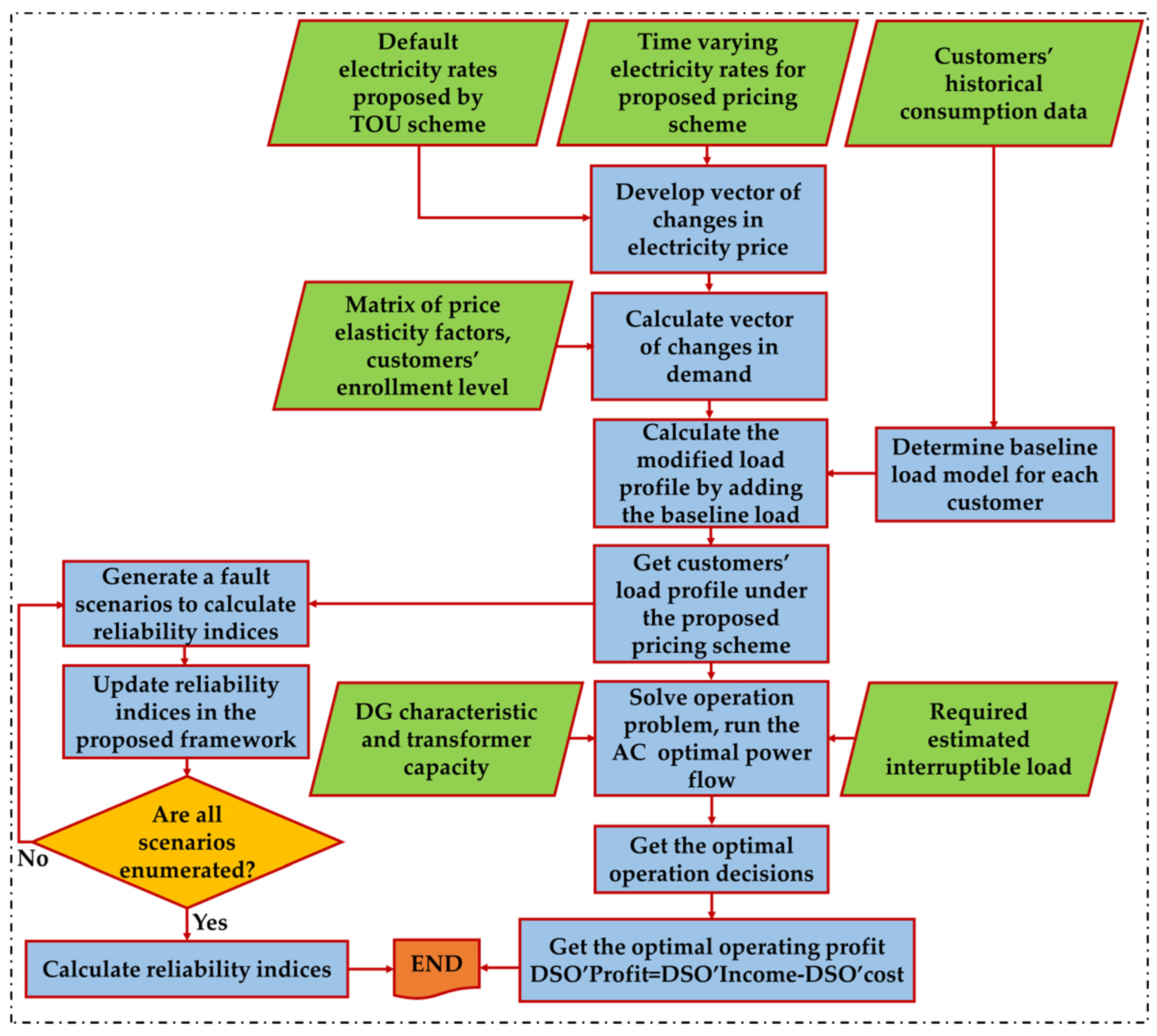
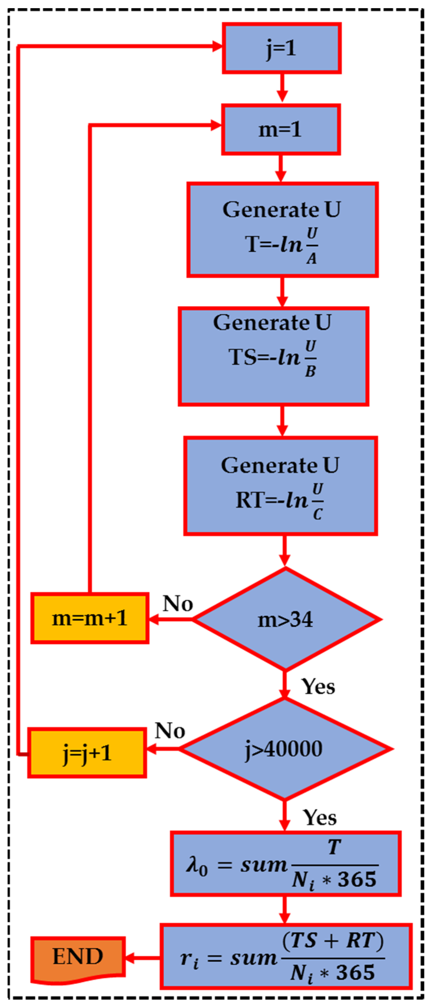
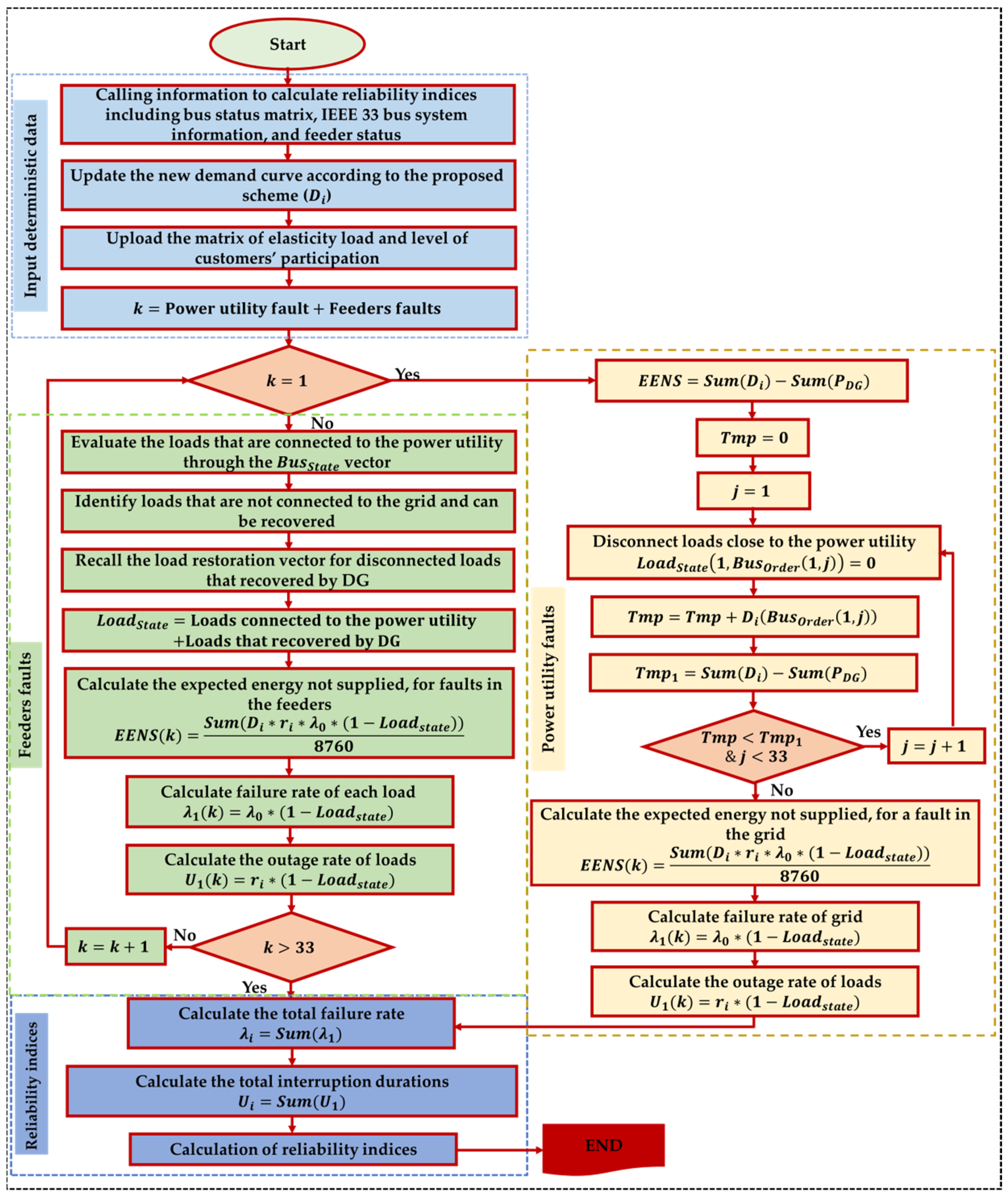
3.3. The Proposed Reliability Evaluation Framework
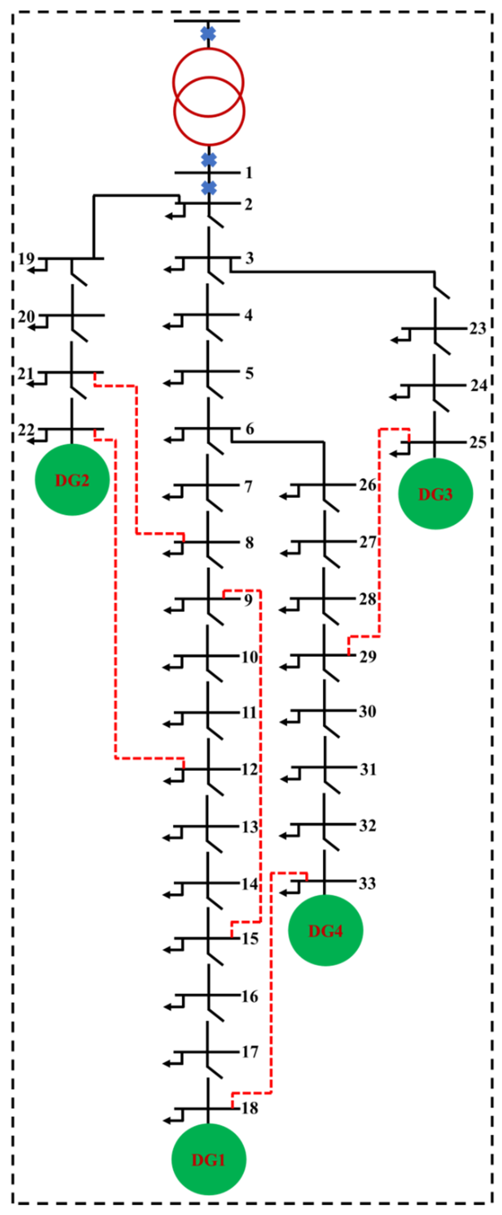
4. Numerical Study
4.1. Short-Term
4.1.1. The First Study
4.1.2. The Second Study
4.1.3. The Third Study
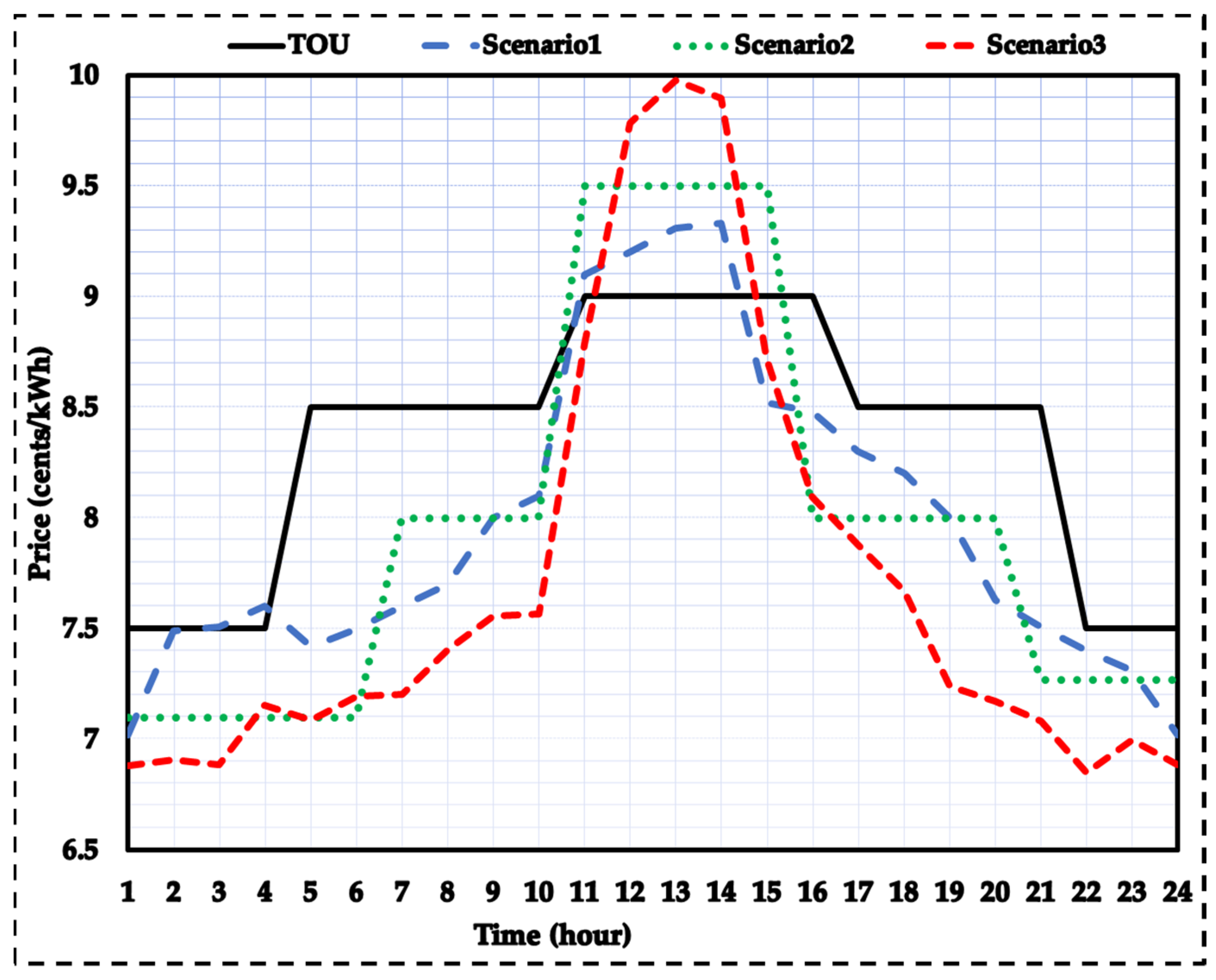
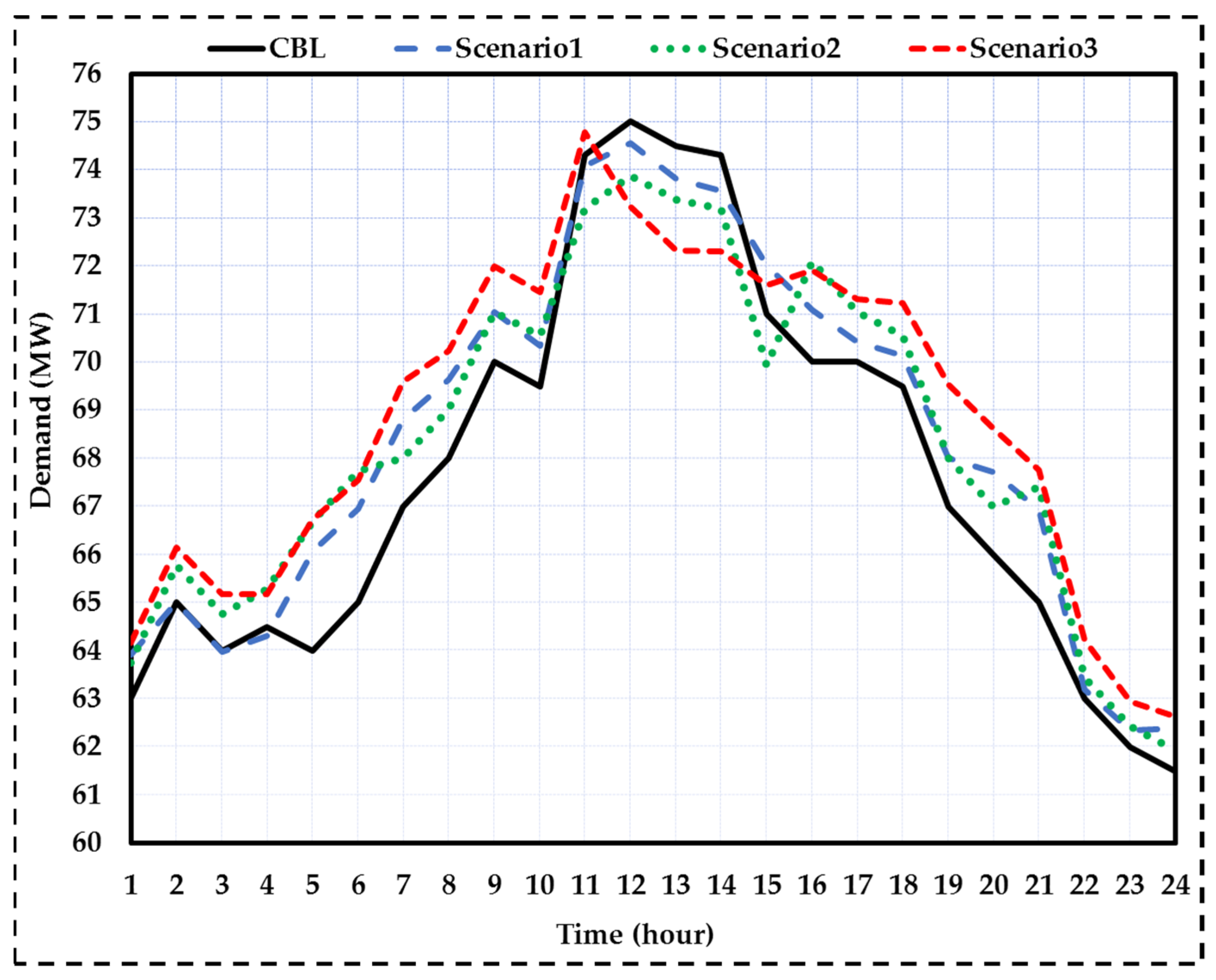
4.1.4. Time-Varying Electricity Rates
4.1.5. Verification of the Results’ Accuracy
4.2. Long-Term
4.2.1. First Case: Calculating Reliability Indices vs. DR Changes
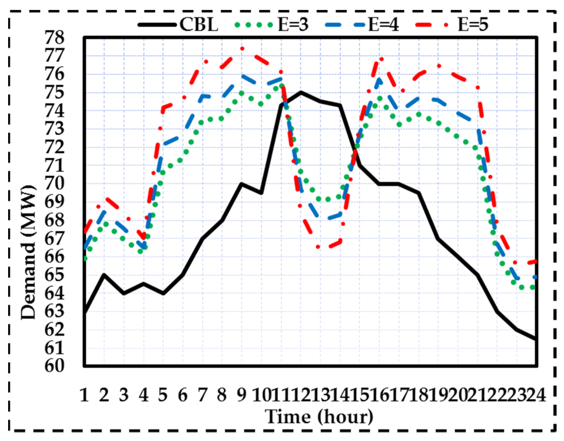
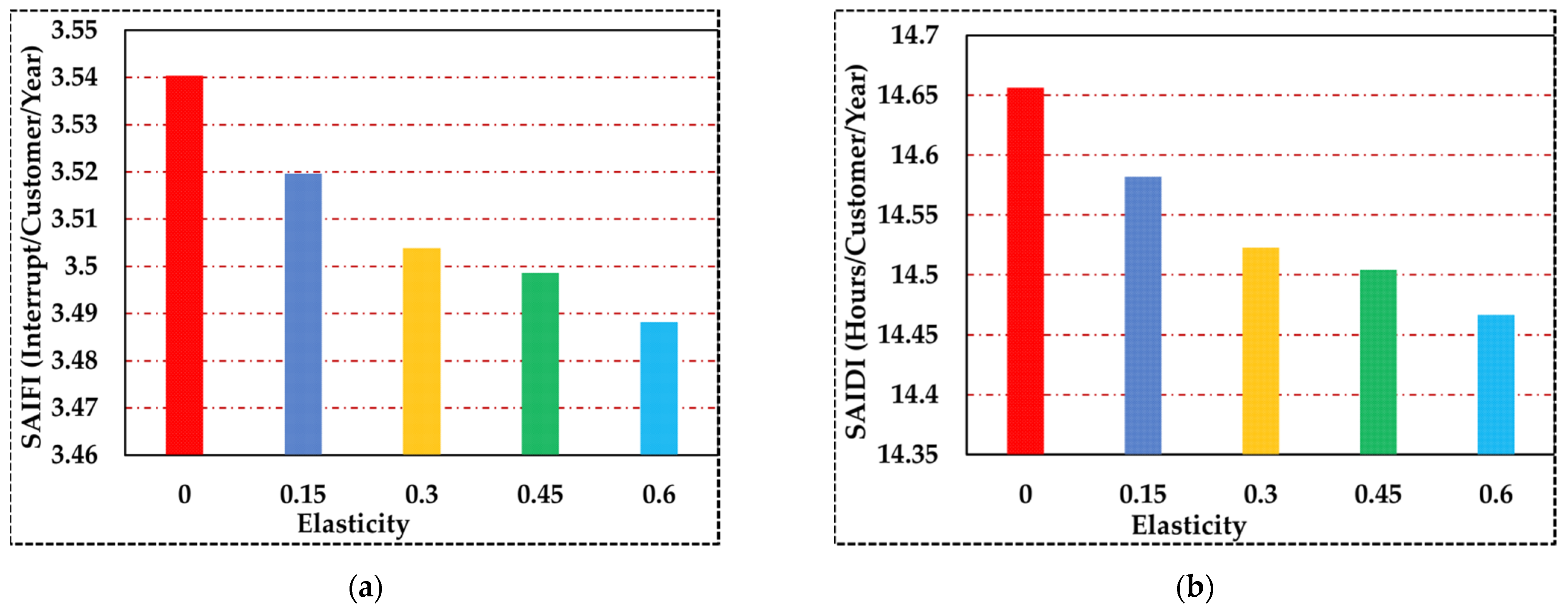
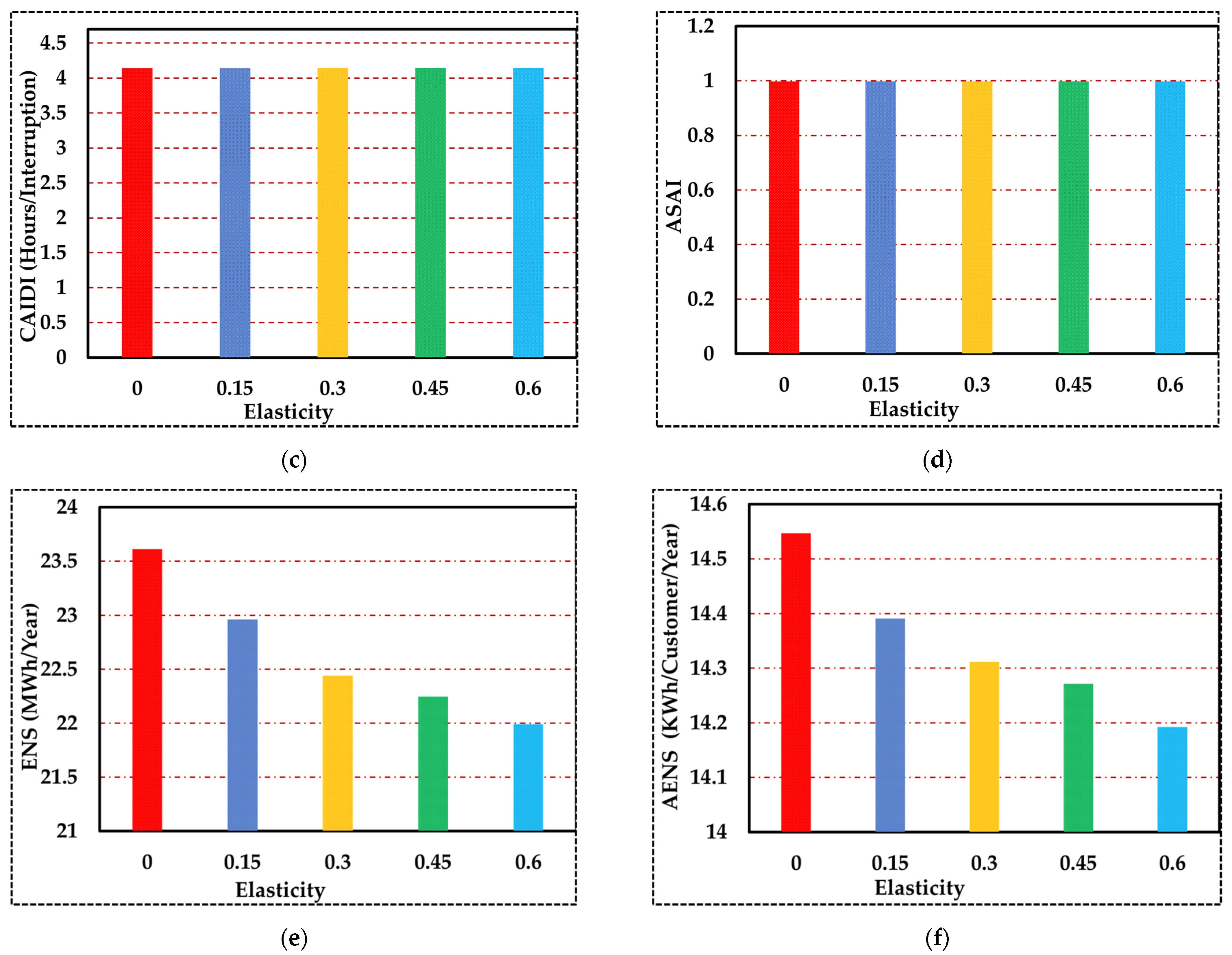
4.2.2. Second Case: Calculating Reliability Indices as Load Elasticity Changes
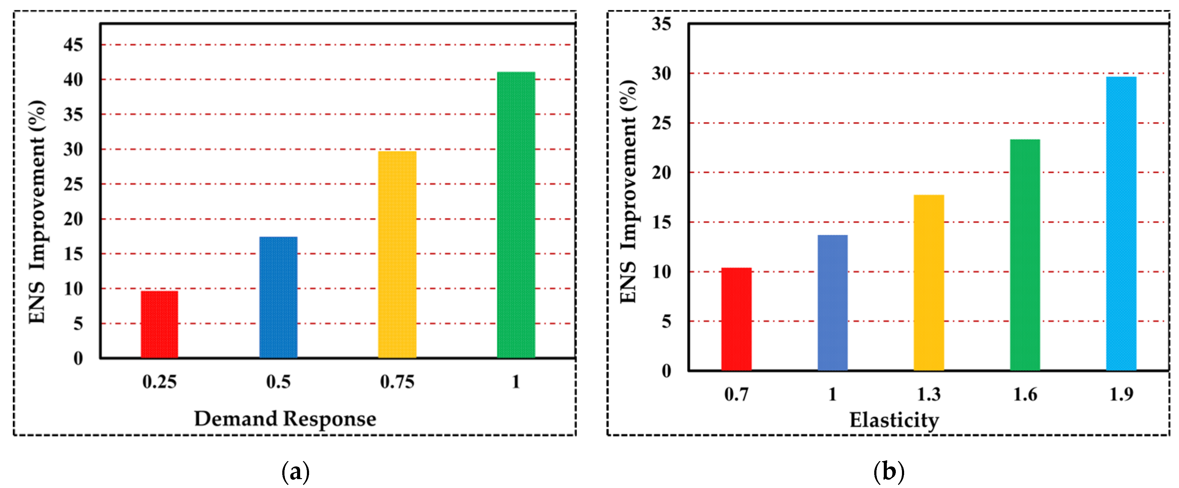
4.3. Sensitivity Analysis of Energy Not Supplied
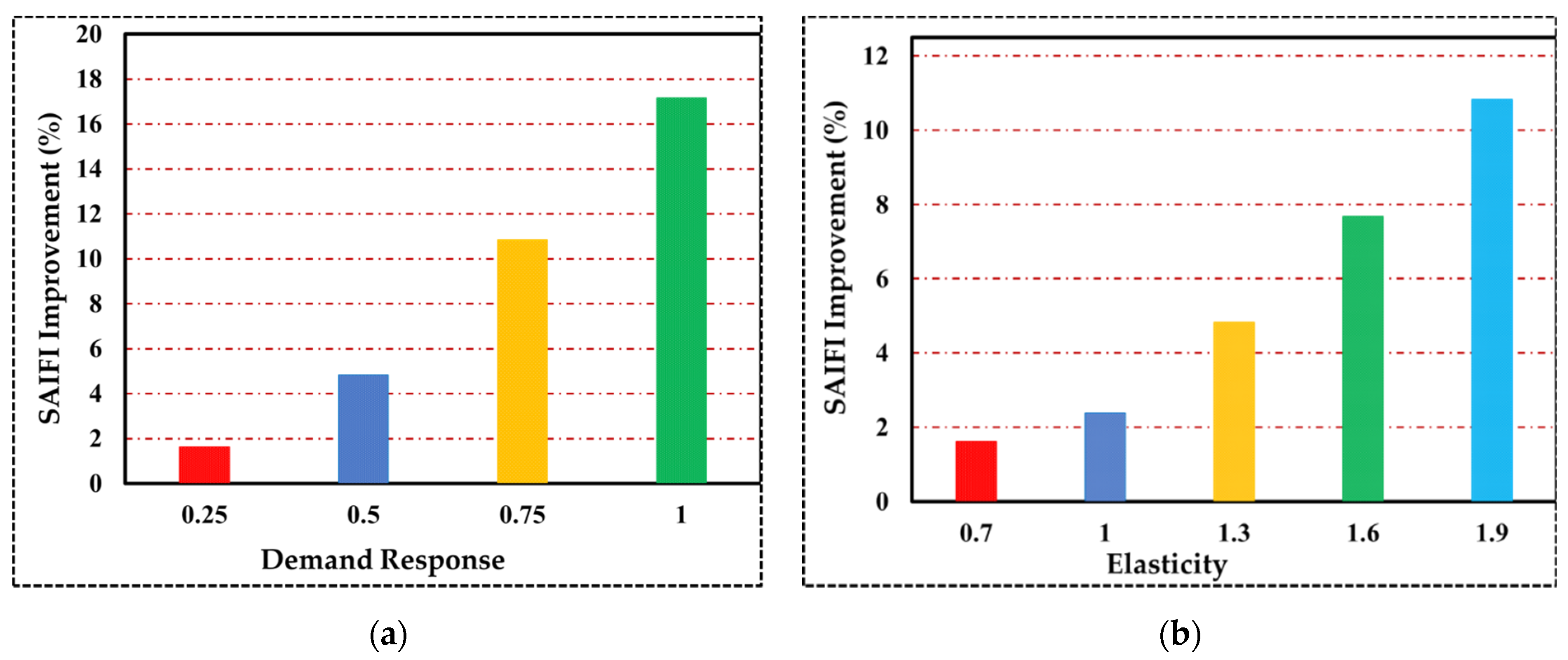
4.4. Sensitivity Analysis of SAIFI
5. Conclusions
Author Contributions
Funding
Institutional Review Board Statement
Informed Consent Statement
Data Availability Statement
Conflicts of Interest
Nomenclature
| A. Indices and Sets | |
| Indices and set of time intervals, running from 1 to T | |
| Indices and set of network buses, running from 1 to 33 | |
| Index and number of distributed generation, running from 1 to 4 | |
| Index of total time (24 h a day) | |
| Set of linear model segments, running from 1 to 10 | |
| Set of different customers from 1 to 3 | |
| B. Parameters and Variables | |
| Binary indicator denoting of the consumption peak hour, equal to 1 on peak, otherwise 0 | |
| Baseline rate, charge rate, credit rate, marginal price, and interruptible load price (USD/MWh) | |
| Minimum up and down time of DG unit (h) | |
| Maximum and minimum of DG capacity limit for activepower (KW) | |
| Maximum capacity of DG generation segment (KW) | |
| DG startup cost parameter (USD) | |
| Binary variable denoting commitment status of DG unit g at time t, equal to 1 if unit g is scheduled to be committed, otherwise 0 | |
| Ramping-up and ramping- down rates ofDG unit g (KW) | |
| Linear generation cost model parameter ofDG unit (USD/KWh) | |
| Minimum generation cost of unit g (USD/KWh) | |
| Price elasticity coefficient, matrix of price elasticity factors, customers’ enrollment level on DR program | |
| Demand of customer j at time t before implementing DR program (MW) | |
| Initial value of electricity price offered tocustomer j at time t (USD) | |
| Cost of using smart measurement infrastructure (USD) | |
| Maximum real power procured from outside grid (MW) | |
| Upper and lower allowed voltage magnitudes (pu) | |
| Linearization constants (radian) | |
| (radian) | |
| Line conductance and susceptance (from bus k to r) (ohm) | |
| Voltage magnitude (voltage angle) at node k at time t (pu) | |
| Constant parameters for distribution function probability | |
| load point (MW) | |
| Failure rate, average repair time, average annual disconnection time (h) | |
| load point, running from 1 to 34 | |
| Active (reactive) power flow from node k to r (MW) | |
| Total bill received from all customers at time t (USD) | |
| Cost of supplying the DS energy at a specific hour (USD) | |
| Power consumption of customers that participate (do not participate) in the proposed scheme (MW) | |
| Active (reactive) power consumed by customers in period. MW (MVAR) | |
| Active (reactive) power generated by each DG unit. KW (KVAR) | |
| Active (reactive) power of interruptible load. MW (MVAR) | |
| Active (reactive) power purchased from grid. MW (MVAR) | |
| Matrix of changes in demand (MW) | |
| Price change vector (USD) | |
| The DSO profit from daily operation (USD) | |
| Piecewise linear cost function of energy generation by DGs (USD) | |
| Power generation for DG g for segment n of piecewise linear cost function. (KW) | |
| Startup cost of DG unit g (USD) | |
| Repair time, switching time (h) | |
| New demand for each bus (MW) | |
| C. Abbreviations | |
| System average interruption frequency index | |
| System average interruption duration index | |
| Customer average interruption duration index | |
| Average service availability index | |
| Average service unavailability index | |
| Average energy not supplied | |
| Energy not supplied | |
| Expected energy not supplied | |
| Customer baseline load (MW) | |
| Demand from customers that participate in the DR program (MW) | |
| Distributed generation | |
| Demand response | |
| Particle swarm optimization | |
| Distribution system | |
| Monte Carlo simulation | |
| Bus state | |
| Load state | |
| Bus order | |
| Mixed integer linear programming model | |
| Real-time pricing | |
| Microgrid | |
| Distribution system operator | |
| Interruptible load | |
| Demand response aggregators | |
| RTM | Real-time market |
| CCP | Critical peak pricing |
| TOU | Time of use |
| RTP | Real time pricing |
| AMI | Advanced metering infrastructure |
| IOT | Internet of things |
References
- Gholami, A.; Shekari, T.; Grijalva, S. Proactive management of microgrids for resiliency enhancement: An adaptive robust approach. IEEE Trans. Sustain. Energy 2017, 10, 470–480. [Google Scholar] [CrossRef]
- Rashidizadeh-Kermani, H.; Vahedipour-Dahraie, M.; Shafie-Khah, M.; Catalao, J.P. A bi-level risk-constrained offering strategy of a wind power producer considering demand side resources. Int. J. Electr. Power Energy Syst. 2019, 104, 562–574. [Google Scholar] [CrossRef]
- Algarni, A.S.; Bhattacharya, K. A Generic Operations Framework for Discos in Retail Electricity Markets. IEEE Trans. Power Syst. 2009, 24, 356–367. [Google Scholar] [CrossRef]
- Jesus, P.D.; De Leão, M.P.; Yusta, J.M.; Khodr, H.M.; Urdaneta, A.J. Uniform marginal pricing for the remuneration of distribution networks. IEEE Trans. Power Syst. 2005, 20, 1302–1310. [Google Scholar]
- Safdarian, A.; Fotuhi-Firuzabad, M.; Lehtonen, M. Integration of price-based demand response in DisCos’ short-term decision model. IEEE Trans. Smart Grid 2014, 5, 2235–2245. [Google Scholar] [CrossRef]
- Parvania, M.; Fotuhi-Firuzabad, M. Integrating load reduction into wholesale energy market with application to wind power integration. IEEE Syst. J. 2011, 6, 35–45. [Google Scholar] [CrossRef]
- Sioshansi, R. Evaluating the impacts of real-time pricing on the cost and value of wind generation. IEEE Trans. Power Syst. 2009, 25, 741–748. [Google Scholar] [CrossRef]
- Chiu, W.Y.; Sun, H.; Poor, H.V. Energy imbalance management using a robust pricing scheme. IEEE Trans. Smart Grid 2012, 4, 896–904. [Google Scholar] [CrossRef] [Green Version]
- Pillay, A.; Karthikeyan, S.P.; Kothari, D.P. Congestion management in power systems–A review. Int. J. Electr. Power Energy Syst. 2015, 70, 83–90. [Google Scholar] [CrossRef]
- Abapour, S.; Nojavan, S.; Abapour, M. Multi-objective short-term scheduling of active distribution networks for benefit maximization of DisCos and DG owners considering demand response programs and energy storage system. J. Mod. Power Syst. Clean Energy 2018, 6, 95–106. [Google Scholar] [CrossRef] [Green Version]
- Narain, A.; Srivastava, S.K.; Singh, S.N. Congestion management approaches in restructured power system: Key issues and challenges. Electr. J. 2020, 33, 106715. [Google Scholar] [CrossRef]
- Safdar, M.; Hussain, G.A.; Lehtonen, M. Costs of demand response from residential customers’ perspective. Energies 2019, 12, 1617. [Google Scholar] [CrossRef] [Green Version]
- Zhou, S.; Zou, F.; Wu, Z.; Gu, W.; Hong, Q.; Booth, C. A smart community energy management scheme considering user dominated demand side response and P2P trading. Int. J. Electr. Power Energy Syst. 2020, 114, 105378. [Google Scholar] [CrossRef]
- Henríquez, R.; Wenzel, G.; Olivares, D.E.; Negrete-Pincetic, M. Participation of demand response aggregators in electricity markets: Optimal portfolio management. IEEE Trans. Smart Grid 2017, 9, 4861–4871. [Google Scholar] [CrossRef]
- Imani, M.H.; Niknejad, P.; Barzegaran, M.R. The impact of customers’ participation level and various incentive values on implementing emergency demand response program in microgrid operation. Int. J. Electr. Power Energy Syst. 2018, 96, 114–125. [Google Scholar] [CrossRef]
- Chen, B.; Ye, Z.; Chen, C.; Wang, J. Toward a MILP modeling framework for distribution system restoration. IEEE Trans. Power Syst. 2018, 34, 1749–1760. [Google Scholar] [CrossRef]
- Haghifam, S.; Dadashi, M.; Zare, K.; Seyedi, H. Optimal operation of smart distribution networks in the presence of demand response aggregators and microgrid owners: A multi follower Bi-Level approach. Sustain. Cities Soc. 2020, 55, 102033. [Google Scholar] [CrossRef]
- Ghasemi, H.; Aghaei, J.; Gharehpetian, G.B.; Safdarian, A. MILP model for integrated expansion planning of multi-carrier active energy systems. IET Gener. Transm. Distrib. 2019, 13, 1177–1189. [Google Scholar] [CrossRef]
- Moghimi, F.H.; Barforoushi, T. A short-term decision-making model for a price-maker distribution company in wholesale and retail electricity markets considering demand response and real-time pricing. Int. J. Electr. Power Energy Syst. 2020, 117, 105701. [Google Scholar] [CrossRef]
- Khalkhali, H.; Hosseinian, S.H. Novel residential energy demand management framework based on clustering approach in energy and performance-based regulation service markets. Sustain. Cities Soc. 2019, 45, 628–639. [Google Scholar] [CrossRef]
- Damisa, U.; Nwulu, N.I.; Sun, Y. Microgrid energy and reserve management incorporating prosumer behind-the-meter resources. IET Renew. Power Gener. 2018, 12, 910–919. [Google Scholar] [CrossRef]
- Vahedipour-Dahraei, M.; Najafi, H.R.; Anvari-Moghaddam, A.; Guerrero, J.M. Security-constrained unit commitment in AC microgrids considering stochastic price-based demand response and renewable generation. Int. Trans. Electr. Energy Syst. 2018, 28, e2596. [Google Scholar] [CrossRef]
- Vahedipour-Dahraie, M.; Najafi, H.R.; Anvari-Moghaddam, A.; Guerrero, J.M. Study of the effect of time-based rate demand response programs on stochastic day-ahead energy and reserve scheduling in islanded residential microgrids. Appl. Sci. 2017, 7, 378. [Google Scholar] [CrossRef] [Green Version]
- Vahedipour-Dahraie, M.; Rashidizadeh-Kermani, H.; Najafi, H.R.; Anvari-Moghaddam, A.; Guerrero, J.M. Stochastic security and risk-constrained scheduling for an autonomous microgrid with demand response and renewable energy resources. IET Renew. Power Gener. 2017, 11, 1812–1821. [Google Scholar] [CrossRef]
- Safdarian, A.; Fotuhi-Firuzabad, M.; Lehtonen, M. Benefits of demand response on operation of distribution networks: A case study. IEEE Syst. J. 2014, 10, 189–197. [Google Scholar] [CrossRef]
- Safdarian, A.; Fotuhi-Firuzabad, M.; Lehtonen, M. Demand response from residential consumers: Potentials, barriers, and solutions. In Smart Grids and Their Communication Systems; Springer: Singapore, 2019; pp. 255–279. [Google Scholar]
- Lee, J.; Yoo, S.; Kim, J.; Song, D.; Jeong, H. Improvements to the customer baseline load (CBL) using standard energy consumption considering energy efficiency and demand response. Energy 2018, 144, 1052–1063. [Google Scholar] [CrossRef]
- Xu, Z.; Gao, Y.; Hussain, M.; Cheng, P. Demand side management for smart grid based on smart home appliances with renewable energy sources and an energy storage system. Math. Probl. Eng. 2020, 2020, 9545439. [Google Scholar] [CrossRef]
- Narimani, M.R. Demand Side Management for Homes in Smart Grids. In Proceedings of the 2019 North American Power Symposium (NAPS), Wichita, KS, USA, 13–15 October 2019; pp. 1–6. [Google Scholar]
- Feng, J.; Zeng, B.; Zhao, D.; Wu, G.; Liu, Z.; Zhang, J. Evaluating demand response impacts on capacity credit of renewable distributed generation in smart distribution systems. IEEE Access 2017, 6, 14307–14317. [Google Scholar] [CrossRef]
- Popović, Ž.; Knezević, S.; Brbaklić, B. Optimal reliability improvement strategy in radial distribution networks with island operation of distributed generation. IET Gener. Transm. Distrib. 2018, 12, 78–87. [Google Scholar] [CrossRef]
- Farzin, H.; Fotuhi-Firuzabad, M.; Moeini-Aghtaie, M. Role of outage management strategy in reliability performance of multi-microgrid distribution systems. IEEE Trans. Power Syst. 2017, 33, 2359–2369. [Google Scholar] [CrossRef]
- Hashemi-Dezaki, H.; Agah, S.M.M.; Askarian-Abyaneh, H.; Haeri-Khiavi, H. Sensitivity analysis of smart grids reliability due to indirect cyber-power interdependencies under various DG technologies, DG penetrations, and operation times. Energy Convers. Manag. 2016, 108, 377–391. [Google Scholar] [CrossRef]
- Hashemi-Dezaki, H.; Askarian-Abyaneh, H.; Haeri-Khiavi, H. Impacts of direct cyber-power interdependencies on smart grid reliability under various penetration levels of microturbine/wind/solar distributed generations. IET Gener. Transm. Distrib. 2016, 10, 928–937. [Google Scholar] [CrossRef]
- Escalera, A.; Hayes, B.; Prodanovic, M. Analytical method to assess the impact of distributed generation and energy storage on reliability of supply. CIRED-Open Access Proc. J. 2017, 2017, 2092–2096. [Google Scholar] [CrossRef] [Green Version]
- Du, S.; Zio, E.; Kang, R. A new analytical approach for interval availability analysis of Markov repairable systems. IEEE Trans. Reliab. 2017, 67, 118–128. [Google Scholar] [CrossRef]
- Wang, X.; Karki, R. Exploiting PHEV to augment power system reliability. IEEE Trans. Smart Grid 2016, 8, 2100–2108. [Google Scholar] [CrossRef]
- Hashemi-Dezaki, H.; Hamzeh, M.; Askarian-Abyaneh, H.; Haeri-Khiavi, H. Risk management of smart grids based on managed charging of PHEVs and vehicle-to-grid strategy using Monte Carlo simulation. Energy Convers. Manag. 2015, 100, 262–276. [Google Scholar] [CrossRef]
- Fünfgeld, S.; Holzäpfel, M.; Frey, M.; Gauterin, F. Stochastic forecasting of vehicle dynamics using sequential monte carlo simulation. IEEE Trans. Intell. Veh. 2017, 2, 111–122. [Google Scholar] [CrossRef]
- Shojaabadi, S.; Abapour, S.; Abapour, M.; Nahavandi, A. Simultaneous planning of plug-in hybrid electric vehicle charging stations and wind power generation in distribution networks considering uncertainties. Renew. Energy 2016, 99, 237–252. [Google Scholar] [CrossRef]
- Moeini-Aghtaie, M.; Farzin, H.; Fotuhi-Firuzabad, M.; Amrollahi, R. Generalized analytical approach to assess reliability of renewable-based energy hubs. IEEE Trans. Power Syst. 2016, 32, 368–377. [Google Scholar] [CrossRef]
- Chen, C.; Wu, W.; Zhang, B.; Singh, C. An analytical adequacy evaluation method for distribution networks considering protection strategies and distributed generators. IEEE Trans. Power Deliv. 2014, 30, 1392–1400. [Google Scholar] [CrossRef]
- Marzband, M.; Azarinejadian, F.; Savaghebi, M.; Guerrero, J.M. An optimal energy management system for islanded microgrids based on multiperiod artificial bee colony combined with Markov chain. IEEE Syst. J. 2015, 11, 1712–1722. [Google Scholar] [CrossRef] [Green Version]
- Aghdam, F.H.; Abapour, M. Reliability and cost analysis of multistage boost converters connected to PV panels. IEEE J. Photovolt. 2016, 6, 981–989. [Google Scholar] [CrossRef]
- Dong, J.; Gao, F.; Guan, X.; Zhai, Q.; Wu, J. Storage-reserve sizing with qualified reliability for connected high renewable penetration micro-grid. IEEE Trans. Sustain. Energy 2016, 7, 732–743. [Google Scholar] [CrossRef]
- Sun, S.; Yang, Q.; Yan, W. A novel Markov-based temporal-SoC analysis for characterizing PEV charging demand. IEEE Trans. Ind. Inform. 2017, 14, 156–166. [Google Scholar] [CrossRef]
- Iversen, E.B.; Møller, J.K.; Morales, J.M.; Madsen, H. Inhomogeneous Markov models for describing driving patterns. IEEE Trans. Smart Grid 2016, 8, 581–588. [Google Scholar] [CrossRef] [Green Version]
- Farzin, H.; Fotuhi-Firuzabad, M.; Moeini-Aghtaie, M. Reliability studies of modern distribution systems integrated with renewable generation and parking lots. IEEE Trans. Sustain. Energy 2016, 8, 431–440. [Google Scholar] [CrossRef]
- Reigosa, P.D.; Wang, H.; Yang, Y.; Blaabjerg, F. Prediction of bond wire fatigue of IGBTs in a PV inverter under a long-term operation. IEEE Trans. Power Electron. 2015, 31, 7171–7182. [Google Scholar]
- Sekhavatmanesh, H.; Cherkaoui, R. Analytical approach for active distribution network restoration including optimal voltage regulation. IEEE Trans. Power Syst. 2018, 34, 1716–1728. [Google Scholar] [CrossRef] [Green Version]
- Zhu, J.; Yuan, Y.; Wang, W. An exact microgrid formation model for load restoration in resilient distribution system. Int. J. Electr. Power Energy Syst. 2020, 116, 105568. [Google Scholar] [CrossRef]
- Gilani, M.A.; Kazemi, A.; Ghasemi, M. Distribution system resilience enhancement by microgrid formation considering distributed energy resources. Energy 2020, 191, 116442. [Google Scholar] [CrossRef]
- Nozhati, S.; Sarkale, Y.; Chong, E.K.; Ellingwood, B.R. Optimal stochastic dynamic scheduling for managing community recovery from natural hazards. Reliab. Eng. Syst. Saf. 2020, 193, 106627. [Google Scholar] [CrossRef]
- Choopani, K.; Hedayati, M.; Effatnejad, R. Self-healing optimization in active distribution network to improve reliability, and reduction losses, switching cost and load shedding. Int. Trans. Electr. Energy Syst. 2020, 30, e12348. [Google Scholar] [CrossRef]
- Sinishaw, G.Y.; Bantyirga, B.; Abebe, K. Analysis of smart grid technology application for power distribution system reliability enhancement: A case study on Bahir Dar power distribution. Sci. Afr. 2021, 21, e00840. [Google Scholar] [CrossRef]
- López-Prado, J.L.; Vélez, J.I.; Garcia-Llinás, G.A. Reliability Evaluation in Distribution Networks with Microgrids: Review and Classification of the Literature. Energies 2020, 13, 6189. [Google Scholar] [CrossRef]
- Vai, V.; Suk, S.; Lorm, R.; Chhlonh, C.; Eng, S.; Bun, L. Optimal Reconfiguration in Distribution Systems with Distributed Generations Based on Modified Sequential Switch Opening and Exchange. Appl. Sci. 2021, 11, 2146. [Google Scholar] [CrossRef]
- The General Algebraic Modeling System (GAMS) Software. Available online: http://www.gams.com (accessed on 15 September 2021).
- Aljohani, T.; Beshir, M. Distribution system reliability analysis for smart grid applications. Smart Grid Renew. Energy 2017, 8, 240–251. [Google Scholar] [CrossRef] [Green Version]


| Reference | Demand Response Program | Elasticity | Reliability Issue | Power Flow | Pricing Method | Approach | Bill Paid by Customers |
|---|---|---|---|---|---|---|---|
| [4] | Yes | No | No | ACOPF | RTP | NLP | No |
| [5] | Yes | No | Yes | ACOPF | RTP | MILP | Yes |
| [6] | Yes | No | No | DCOPF | TOU | MILP | Yes |
| [7] | Yes | Yes | No | No | RTP | NLP | No |
| [8] | No | No | No | No | Dynamic pricing | LMI | No |
| [9] | Yes | No | No | ACOPF | RTP | Genetic algorithm | No |
| [10] | Yes | No | No | ACOPF | TOU | Fuzzy satisfying | No |
| [11] | Yes | No | No | ACOPF | RTP | MILP | No |
| [12] | Yes | No | No | NO | RTP | LP | Yes |
| [13] | Yes | No | No | ACOPF | No | MILP | No |
| [14] | Yes | No | No | ACOPF | LC | MILP | No |
| [15] | Yes | Yes | No | ACOPF | RTP | NLP | No |
| [16] | No | No | No | ACOPF | No | MILP | No |
| [17] | Yes | No | No | ACOPF | RTP | Big-M method | Yes |
| [18] | Yes | No | No | ACOPF | Various methods | MINLP | No |
| [19] | Yes | Yes | No | ACOPF | RTP | MILP | No |
| [20] | Yes | No | No | ACOPF | RTP | NLP | No |
| [21] | No | No | No | ACOPF | Prices | MILP | No |
| [22] | Yes | Yes | No | ACOPF | RTP | MILP | No |
| [23] | Yes | Yes | No | ACOPF | Dynamic pricing | MILP | No |
| [24] | Yes | Yes | No | ACOPF | RTP | MILP | Yes |
| [25] | Yes | No | Yes | ACOPF | Prices | NLP | No |
| [26] | Yes | No | No | ACOPF | TOU | MILP | Yes |
| [27] | Yes | No | No | No | No | NLP | No |
| [28] | No | No | Yes | ACOPF | RTP | NLP | No |
| [29] | Yes | No | No | DCOPF | RTP | MILP | No |
| [30] | Yes | No | No | No | No | Fuzzy model | No |
| [31] | Yes | No | No | ACOPF | No | MILP | No |
| [32,35,36,37,38,39,40] | No | No | Yes | OPF | No | Monte Carlo simulation | No |
| [43,45,47] | No | No | Yes | ACOPF | No | Markov method | No |
| [46,48,49] | No | No | Yes | No | No | Monte Carlo simulation | No |
| [51] | No | No | Yes | ACOPF | No | MINLP | No |
| [52] | Yes | No | Yes | ACOPF | No | MILP | No |
| [53] | No | No | Yes | ACOPF | No | Rollout algorithm | No |
| [54] | No | No | No | No | No | PSO algorithm | No |
| This paper | Yes | Yes | Yes | ACOPF | RTP | MILP | Yes |
| Proposed Scheme (USD) | Present RTP (USD) | |
|---|---|---|
| Best scenario payment | 1.3774 × 10⁵ | 1.3129 × 10⁵ |
| Worst scenario payment | 1369 × 105 | 1.279 × 10⁵ |
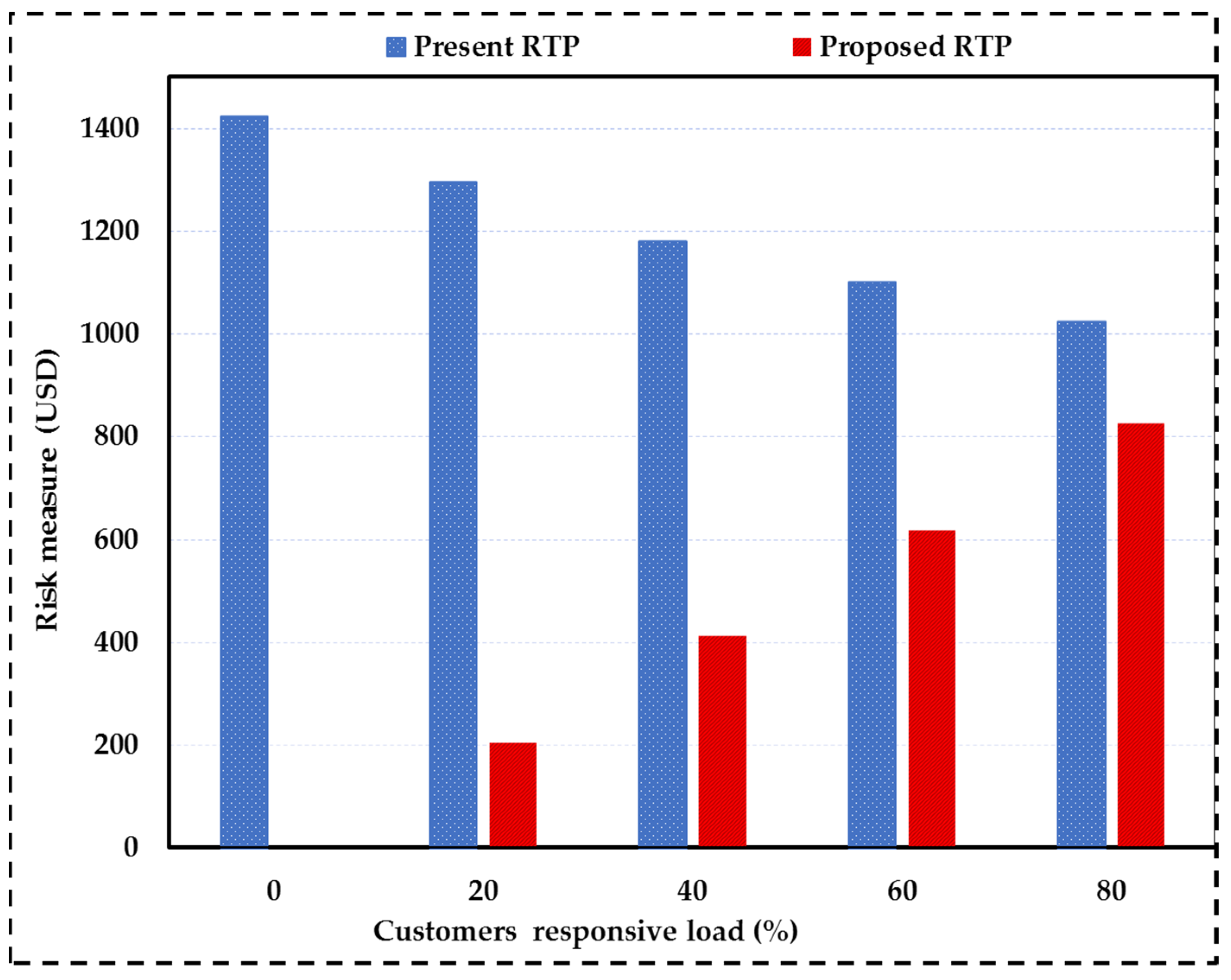
| Payment exposure risk | 516.54 | 1140.8 |
| Pricing Scheme | DSO Income | Purchase from Grid | IL Purchase | DG Generation | DSO Profit |
|---|---|---|---|---|---|
| Existing present RTP scheme | 131,287 | 96,788 | 160.566 | 14,320.00 | 20,018.2 |
| The proposed RTP scheme | 137,023 | 96,788 | 160.566 | 14,320.00 | 25,754 |
| Pricing Scheme | Enrollment Level | (USD) | (USD) | (USD) | (USD) | (USD) |
|---|---|---|---|---|---|---|
| Existing RTP scheme | 0 | 135,729 | 95,391.42 | 383.057 | 14,320 | 25,634.52 |
| Proposed RTP scheme | 0 | 129,993 | 94,391.42 | 383.057 | 14,320 | 19,898.76 |
| DR | (USD) | (USD) | (USD) | (USD) | (USD) | Improvement (%) |
|---|---|---|---|---|---|---|
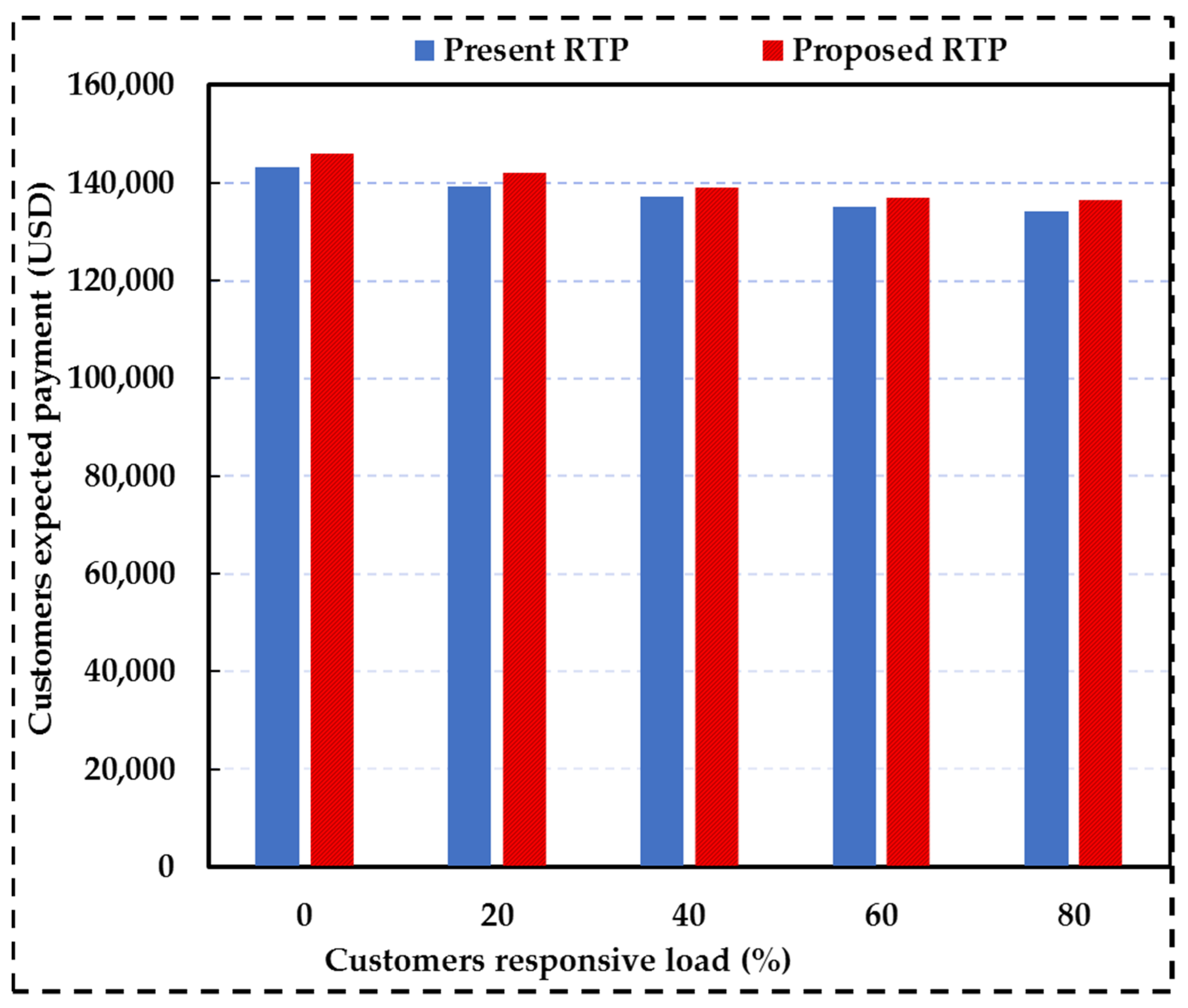
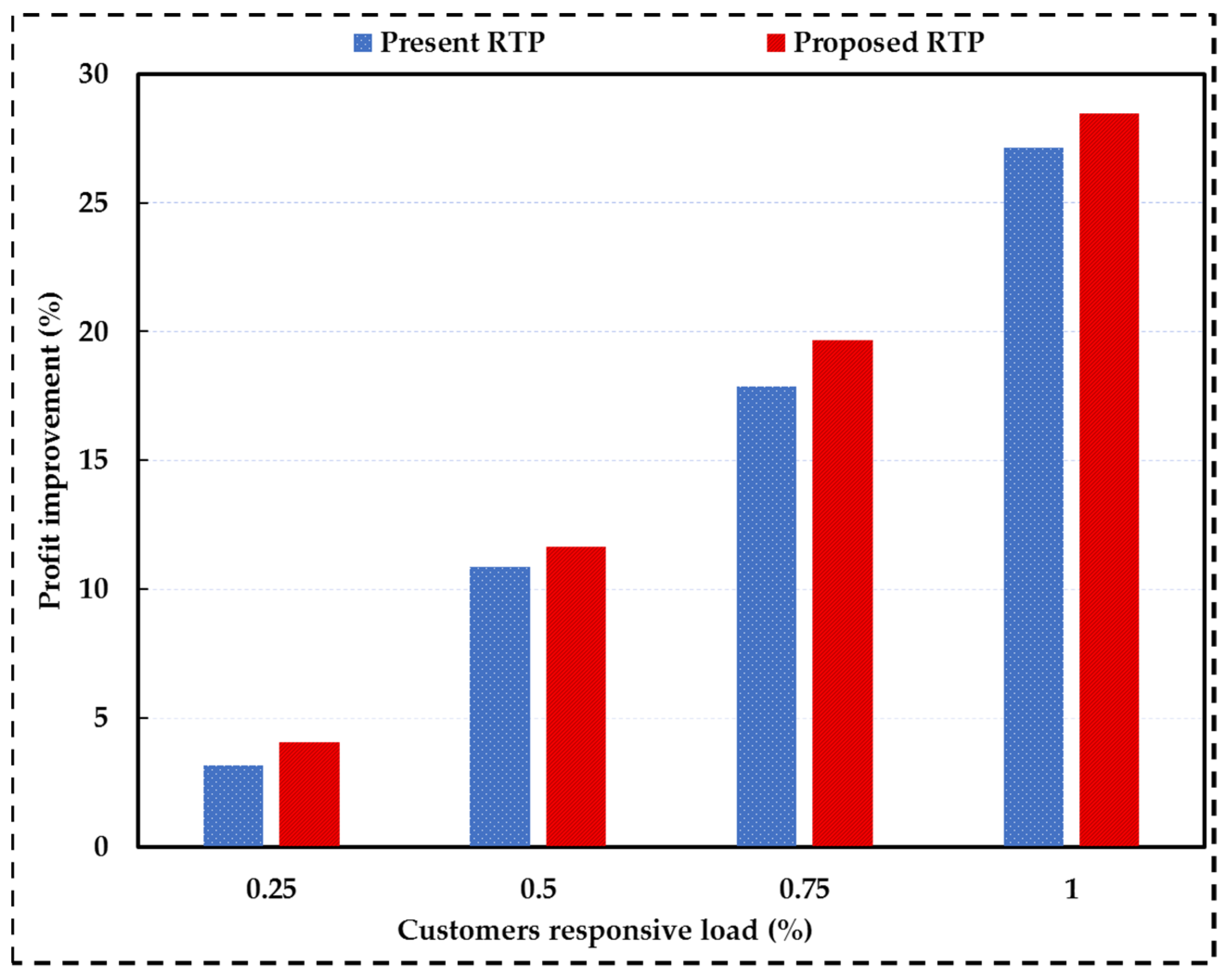
| 25% | 136,160.2 | 94,858.56 | 305.564 | 14,320 | 26,676.1 | 4.0631773 |
| 50% | 136,591.4 | 93,425.6 | 228.285 | 14,320 | 28,617.56 | 11.6367851 |
| 75% | 137,022.7 | 92,121.18 | 160.566 | 14,320 | 30,420.92 | 18.6716701 |
| 100% | 137,453.9 | 90,338.57 | 119.006 | 14,320 | 32,676.31 | 27.4699234 |
| E | (USD) | (USD) | (USD) | (USD) | (USD) | Improvement (%) |
|---|---|---|---|---|---|---|
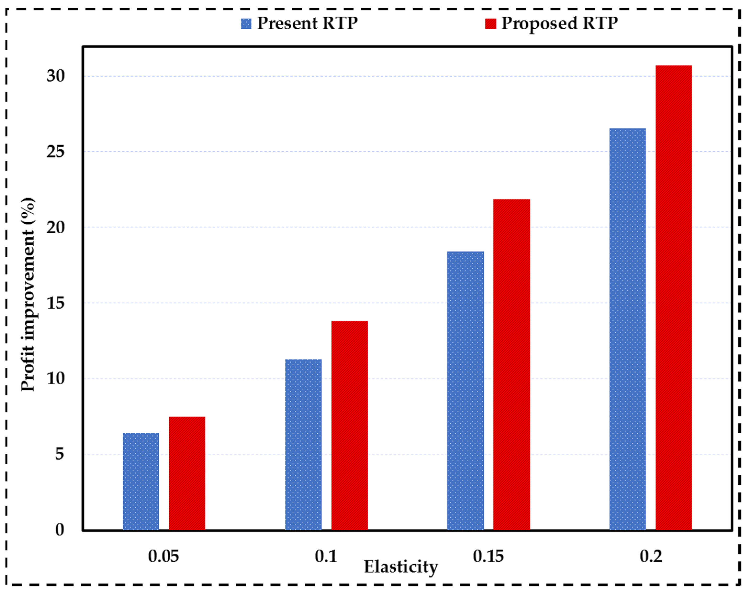
| 0.05 | 136,591.4 | 94,375.1 | 344.203 | 14,320 | 27,552.2 | 7.481 |
| 0.1 | 137,453.9 | 93,658.6 | 305.564 | 14,320 | 29,169.8 | 13.791 |
| 0.15 | 138,316.3 | 92,492.1 | 266.925 | 14,320 | 31,237.3 | 21.856 |
| 0.2 | 139,178.8 | 91,125.6 | 228.285 | 14,320 | 33,504.9 | 30.702 |
| Electricity Rate | DSO Profit | ||||
|---|---|---|---|---|---|
| TOU | 133,160 | 95,383.1 | 539.9 | 14,320 | 22,917 |
| CPP | 127,822 | 107,557.5 | 541.5 | 14,320 | 5403 |
| RTP | 137,023 | 96,788 | 160.566 | 14,320 | 25,754 |
| Case | Model | Best Solution (USD) | Absolute Gap | Computation Time (Min.) |
|---|---|---|---|---|
| DR = 0, E = 0.04 | MILP | 19,898.76 | 0% | 0.25 |
| DR = 0.25, E = 0.04 | MILP | 26,676.1.6 | 0% | 5 |
| DR = 0.5, E = 0.04 | MILP | 28,617.56 | 0% | 5.09 |
| DR = 0.75, E = 0.04 | MILP | 30,420.92 | 0% | 5.11 |
| Case | Model | Best Solution (USD) | Absolute Gap | Computation Time (Min.) |
|---|---|---|---|---|
| DR = 0, E = 0.04 | MILP | 19,899.8 | 0% | 8 |
| DR = 0.25, E = 0.04 | MILP | 26,677.2 | 0% | 26.4 |
| DR = 0.5, E = 0.04 | MILP | 28,618.6 | 0% | 26.67 |
| DR = 0.75, E = 0.04 | MILP | 30,423 | 0% | 26.78 |
| Reliability Indices | Value |
|---|---|
| SAIFI (interrupt/customer/year) | 3.5404 |
| SAIDI (hours/customer/year) | 14.6565 |
| CAIDI (hours/interruption) | 4.1399 |
| ASAI | 0.9984 |
| ASUI | 0.00165 |
| ENS(MWh/year) | 23.6110 |
| AENS (KWh/customer/year) | 14.5468 |
| Solution Approaches | SAIFI | SAIDI | CAIDI | ASAI |
|---|---|---|---|---|
| Model presented in [55] | 21.5210 | 40.3415 | 1.875 | 0.9985 |
| Model presented in [59] | 5.35187 | 927.25 | 173.25 | 0.9987 |
| Proposed model | 3.5404 | 14.656 | 4.1399 | 0.9984 |
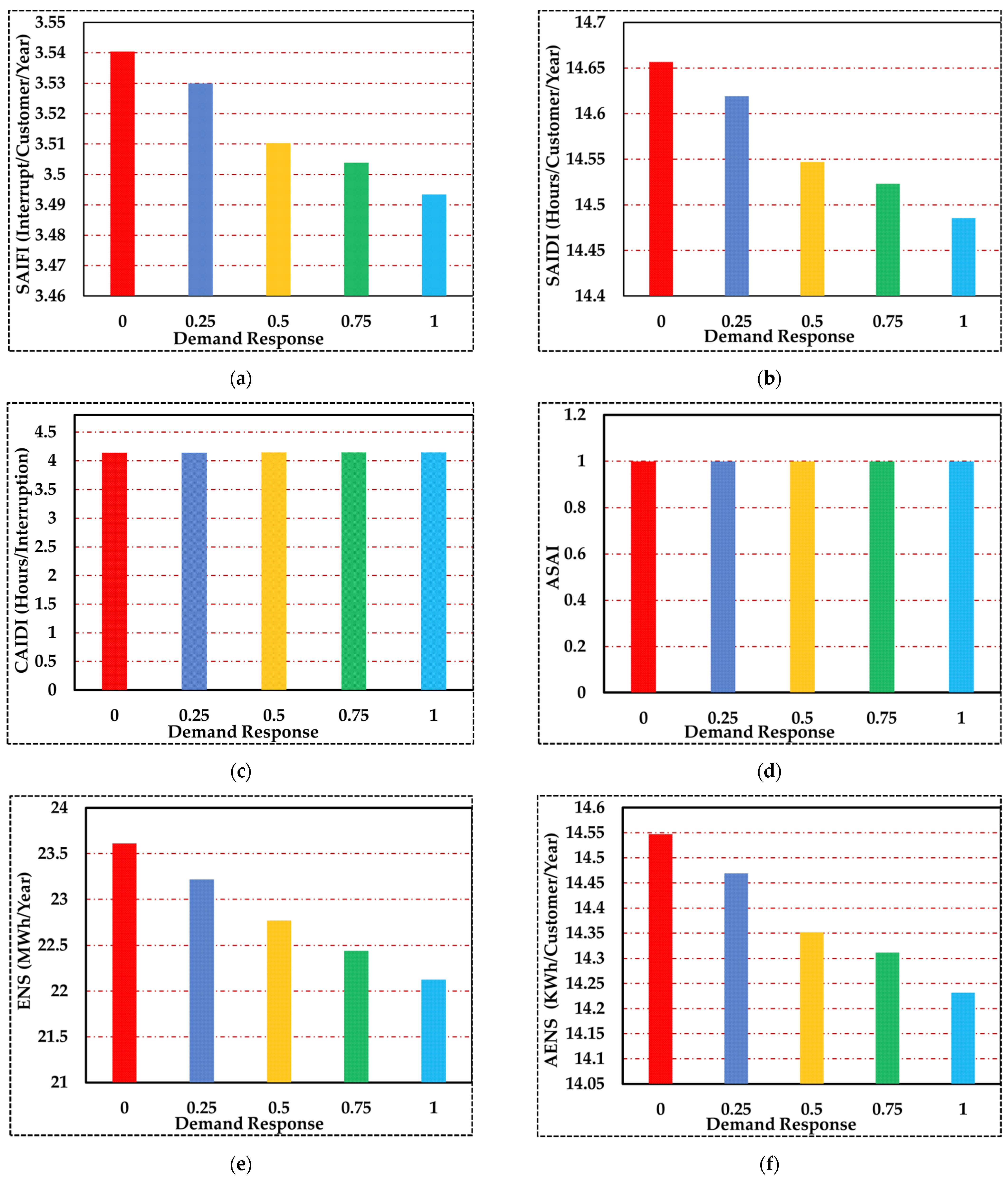
| DR | SAIFI | SAIDI | CAIDI | ASAI | ASUI | ENS | AENS |
|---|---|---|---|---|---|---|---|
| 0 | 3.54038 | 14.6565 | 4.1399 | 0.99835 | 0.001649 | 23.6109 | 14.5468 |
| 0.25 | 3.51957 | 14.5818 | 4.1432 | 0.99835 | 0.001649 | 22.9618 | 14.3912 |
| 0.50 | 3.50378 | 14.5229 | 4.14501 | 0.99835 | 0.001649 | 22.4406 | 14.3117 |
| 0.75 | 3.48817 | 14.4669 | 4.14742 | 0.99835 | 0.001649 | 21.9928 | 14.1924 |
| 1 | 3.48297 | 14.4482 | 4.14823 | 0.99835 | 0.001649 | 21.7581 | 14.1527 |
| Self-Elasticity | SAIFI | SAIDI | CAIDI | ASAI | ASUI | ENS | AENS |
|---|---|---|---|---|---|---|---|
| 0 | 3.5404 | 14.6565 | 4.1399 | 0.9984 | 0.00165 | 23.6110 | 14.5468 |
| 0.15 | 3.5300 | 14.6191 | 4.1416 | 0.9984 | 0.00165 | 23.2183 | 14.4686 |
| 0.30 | 3.5103 | 14.5469 | 4.1441 | 0.9984 | 0.00165 | 22.7673 | 14.3519 |
| 0.45 | 3.5038 | 14.5229 | 4.1450 | 0.9984 | 0.00165 | 22.4405 | 14.3116 |
| 0.60 | 3.4882 | 14.4669 | 4.1474 | 0.9984 | 0.00165 | 21.9928 | 14.1923 |
| Self-Elasticity | DR = 0.25 | DR = 0.50 | DR = 0.75 | DR = 1 |
|---|---|---|---|---|
| 0.7 | 22.6175 | 21.7581 | 21.1515 | 20.5449 |
| 1 | 22.3521 | 21.2382 | 20.3716 | 19.1548 |
| 1.3 | 21.8447 | 20.7182 | 19.4172 | 17.5737 |
| 1.6 | 21.5848 | 20.1983 | 18.0944 | 15.3805 |
| 1.9 | 21.3248 | 19.5021 | 16.6074 | 13.9134 |
| Self-Elasticity | DR = 0.25 | DR = 0.50 | DR = 0.75 | DR = 1 |
|---|---|---|---|---|
| 0.7 | 3.5038 | 3.4830 | 3.4829 | 3.4740 |
| 1 | 3.5038 | 3.4830 | 3.4561 | 3.3494 |
| 1.3 | 3.4829 | 3.4785 | 3.3693 | 3.2340 |
| 1.6 | 3.4829 | 3.4336 | 3.2685 | 3.0606 |
| 1.9 | 3.4829 | 3.3693 | 3.1566 | 2.9329 |
Publisher’s Note: MDPI stays neutral with regard to jurisdictional claims in published maps and institutional affiliations. |
© 2021 by the authors. Licensee MDPI, Basel, Switzerland. This article is an open access article distributed under the terms and conditions of the Creative Commons Attribution (CC BY) license (https://creativecommons.org/licenses/by/4.0/).
Share and Cite
Mansouri, M.R.; Simab, M.; Bahmani Firouzi, B. Impact of Demand Response on Reliability Enhancement in Distribution Networks. Sustainability 2021, 13, 13201. https://doi.org/10.3390/su132313201
Mansouri MR, Simab M, Bahmani Firouzi B. Impact of Demand Response on Reliability Enhancement in Distribution Networks. Sustainability. 2021; 13(23):13201. https://doi.org/10.3390/su132313201
Chicago/Turabian StyleMansouri, Mohammad Reza, Mohsen Simab, and Bahman Bahmani Firouzi. 2021. "Impact of Demand Response on Reliability Enhancement in Distribution Networks" Sustainability 13, no. 23: 13201. https://doi.org/10.3390/su132313201
APA StyleMansouri, M. R., Simab, M., & Bahmani Firouzi, B. (2021). Impact of Demand Response on Reliability Enhancement in Distribution Networks. Sustainability, 13(23), 13201. https://doi.org/10.3390/su132313201