Abstract
Dual-stage standalone photovoltaic (PV) systems suffer from stability, reliability issues, and their efficiency to deliver maximum power is greatly affected by changing environmental conditions. A hybrid back-stepping control (BSC) is a good candidate for maximum power point tracking (MPPT) however, there are eminent steady-state oscillations in the PV output due to BSC’s recursive nature. The issue can be addressed by proposing a hybrid integral back-stepping control (IBSC) algorithm where the proposed integral action significantly reduces the steady-state oscillations in the PV array output under varying temperature and solar irradiance level. Simultaneously, at the AC stage, the primary challenge is to reduce both the steady-state tracking error and total harmonic distortion (THD) at the output of VSI, resulting from the load parameter variations. Although the conventional sliding mode control (SMC) is robust to parameter variations, however, it is discontinuous in nature and inherit over-conservative gain design. In order to address this issue, a dynamic disturbance rejection strategy based on super twisting control (STC) has been proposed where a higher order sliding mode observer is designed to estimate the effect of load disturbances as a lumped parameter which is then rejected by the newly designed control law to achieve the desired VSI tracking performance. The proposed control strategy has been validated via MATLAB Simulink where the system reaches the steady-state in s and gives a DC–DC conversion efficiency of at the peak solar irradiation level. The AC stage steady-state error is minimized to 0 V whereas, THD is limited to and for linear and non-linear loads, respectively.
1. Introduction
Due to the depleting traditional fuel reserves and serious environmental concerns related to them, sustainable energy resources are gradually replacing fossil fuels as a source of energy [1,2,3]. Due to their abundant availability and reusable properties, researchers are becoming more interested in renewable energy sources, such as wind, hydro, and solar energy. Solar energy is considered among the rapidly growing technologies and has also experienced a significant decline in cost over the past decade [4,5,6]. In addition to its cost-effectiveness advantage, solar photovoltaic (PV) systems generate noise free electricity, produce no environmental pollution, do not deplete natural resources and is relatively easy to assemble. However, the major drawbacks of PV systems are their highly non-linear dynamics, low efficiency, and environment-dependent characteristics. Studies report that the efficiency of PV cells can range from to only, and the power supplied by the PV system varies continuously with varying solar irradiation levels and surrounding temperatures [7]. Several solutions are proposed in the literature to improve the performance and efficiency of PV systems in order to achieve a consistent and reliable power output particularly, in changing environmental conditions. The maximum power point tracking (MPPT) techniques represent one of the most convenient solution to reach and maintain the optimal operating point in the PV module. These techniques use DC–DC power converters and a control algorithm that generates the duty ratio of that power converter in such a way that the PV array and converter impedance are matched and the maximum power can be extracted. The most common algorithm employed in this regard is perturb and observe (P&O) based algorithm, in which the output voltage of PV module is perturbed and the change in output power is observed. If the change in power, , then the voltage will be further perturbed in the same direction until and vice versa [8]. In [9], the P&O parameters are optimized at the same pattern to generate the duty ratio for the converter switch to attain maximum power point (MPP). As the algorithm makes periodic changes in voltage and duty ratio of the boost converter to track the MPP, therefore, it creates an oscillatory operating point. To overcome the oscillatory nature of MPP in P&O, incremental conductance (IC) algorithm has been presented in [10,11,12]. The strategy utilizes the current and voltage measurements to determine the trajectory of working point thus, giving better performance for uniform weather conditions. However, when the atmospheric conditions are varied, the tracking becomes exponentially harder because of continuous change in the slope of the PV curve [3]. Both of these classical algorithms have the common problem of oscillations around the operating point in the steady-state because of atmospheric changes [13]. These oscillations in the output not only cause power losses in the DC stage but also affect the output of the next AC stage when used in coupled mode.
In order to remove the steady-state oscillations around MPP and to achieve better efficiency in a shorter response time, intelligent controllers, such as fuzzy logic and artificial neural network (ANN)-based algorithms have been proposed in [14,15] to track the MPP. These non-linear techniques are not only robust and efficient but also do not require any system knowledge to perform their operation. However, on the downside, the performance of fuzzy based systems and its computational complexity rely on an adapted fuzzy model based on the system’s behaviour in varying environment [16]. On the other hand, ANN require rigorous training mechanism to perform their operation under varying environmental conditions. Among the category of intelligent techniques, optimization based algorithms, such as genetic algorithm (GA) [17], grey wolf optimization (GWO) [18], aunt colony optimization (ACO) [19], particle swarm optimization (PSO) [20], and musical chairs algorithm [21] are proved more efficient when compared with conventional algorithms specifically under partial shading conditions. These algorithms rely on the bio-inspired population which is initialized randomly where, each member of the population presents a solution that is communicated among the population to reach the global maximum power point. However, these techniques continuously evaluate the possible solutions, which makes their convergence response slow.
In addition to these techniques, other non-linear tracking techniques have been proposed to track the MPP with improved accuracy, such as sliding mode control (SMC) [11,22] and back-stepping control (BSC) [23]. SMC is well suited for variable structure systems and inherits the properties of robustness and tolerance against external disturbances but it suffers from chattering. The BSC control proved stable and efficient for nonlinear systems because of its Lyapunov function-based design criteria. In [8], BSC has been presented for MPP tracking with a buck converter. A similar control scheme has been adapted in [23] for boost converter to track MPP under varying environmental conditions. Although the algorithm proves itself in robustness and efficiency, however, BSC suffers from the complexity of requiring the computation of derivatives of virtual states, which makes such implementations prone to numerical instability [24]. Consequently, a significant steady-state error is observed in the output during MPP tracking. In response to this, researchers have attempted countermeasures, such as filtering the virtual states to address the differential issues of virtual states [25,26]. However, command filters create filter errors that negatively impact the controller’s performance and a filter compensation signal is needed to be designed to eliminate these issues. Another effective way to remove the steady-state oscillations in BSC is the inclusion of integral action. The integral action is applied during the backstepping design process to improve the convergence of steady-state error under varying environmental conditions. To remove the steady-state oscillations in BSC, integral back-stepping control (IBSC) has been presented in [27] for grid-connected distributed generation system. In similar scope of study IBSC has been used in [28] for MPPT extraction with buck-boost operation with an electro-mechanical sound system serving as load. Despite the fact that hybrid IBSC is stable by design and mitigates steady-state fluctuations, there are still limited studies in the existing literature for IBSC based MPPT for standalone PV systems.
At the second stage of the PV control system, the accurate regulation of AC voltage and current is of significant importance. In addition to the nonlinear dynamics of DC–AC voltage source inverter (VSI), the system performance at this stage is sensitive to changes in input voltage levels due to variable irradiance levels and sudden fluctuations in load [29,30]. Any variation in the load acts as a mismatched disturbance entering the system through a channel different from control input, resulting in a periodic error at the inverter output voltage [31]. Additionally, when the inverter is connected to highly non-linear loads, a significant level of total harmonic distortion (THD) is observed at the inverter output voltage. Consequently, the control performance is degraded, which, in turn, triggers problems in the application systems [32,33]. Therefore, in AC stage controller design, it is critical to design a controller that can endure these disturbances with minimal THD and steady-state error characteristics.
SMC gives a robust dynamic response and reduced steady-state error when applied to VSI for reference tracking; however, the crucial problems in traditional SMC are its discontinuous nature and over conservative gain, and design [34,35]. Because of the inherent signum function in the control structure, the control signal oscillates at infinite frequency [36] and results in a high steady-state error and harmonic content in the inverter output. In addition, if the switching gain of SMC, which is designed to overcome the disturbances in the system, is selected arbitrarily large, then it generates a transient response with excessive settling time and an undesirable level of overshoot in the inverter output. Higher order sliding mode control techniques are proposed to address the discontinuous nature of SMC in [37,38], however, the switching gain must be selected greater than the bound of the disturbances to ensure the stability of the PV control system. An effective solution to address this over conservative gain design is a disturbance rejection strategy in which the inverter disturbances are estimated and then subtracted from the system rather than compensating through the SMC switching gain. In [31,39,40], disturbance rejection based SMC strategies have been presented for the smooth operation of the inverter system. Although disturbance rejection based dynamic SMC control schemes exhibit better performance for matched disturbances, the studies in the existing literature with mismatched inverter uncertainties are still limited.
In this paper, a standalone PV system with two independent control strategies have been presented. At the first stage, a hybrid non-linear MPPT technique based on P&O and IBSC algorithm is proposed to extract the maximum power from the PV array. The integral action in the MPPT algorithm significantly reduces the oscillations in the PV array output that is fed to the DC–AC inverter at the second stage. Then, at the second stage, a dynamic disturbance rejection strategy based on super twisting sliding mode control (ST-SMC) is proposed to regulate AC power for a variety of loads at the system output. The PV inverter load parameter disturbances and their effect on the system dynamics are aggregated into a lumped perturbation, which is then estimated online by a newly designed higher-order sliding mode observer. The estimated perturbation is then compensated by the ST-SMC, such that a better control performance could be achieved with significant robustness against load disturbances. The main contributions of the text are listed below
- At the DC stage, the proposed algorithm accurately tracks the MPP, and the MPPT efficiency remains at at the peak solar irradiation level;
- At the AC stage, the controller is model-independent, and only the output voltage measurement is required to implement the proposed dynamic STC;
- The HOSMO proposed is finite-time convergent and gives robust estimates of system states and accumulates the effects of load disturbances as a lumped parameter. The concept of lumped disturbance rejection enhances the effectiveness of the control law.
The effectiveness of proposed algorithm is verified for linear and non-linear loads via MATLAB simulations where, the system is subjected to variable temperature and solar irradiations.
2. DC–DC Stage Modeling
The DC–DC stage consists of PV solar array that is a combination of multiple solar cells and a DC–DC boost converter as illustrated in Figure 1. Modelling of a solar cell can be attained by employing five elements which consist of a photon current source connected in parallel with a diode, a kilo-ohms level shunt resistance and a milli-ohms level series resistance , as presented in Figure 2. Based on the solar irradiance, becomes the source current which is also dependent on the temperature. Thus, the PV output current is actually a function of irradiance and environmental temperature given as
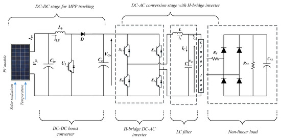
Figure 1.
PV based dual stage generation system.
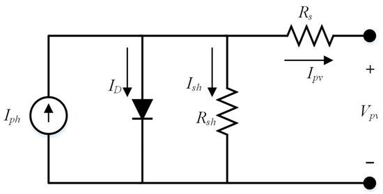
Figure 2.
Structure of the individual solar cell.
The voltage across diode can be written as
Then, the diode current can be written as
where is the diode saturation current and is the thermal voltage given as
where K is Boltsman constant, is the diode ideality factor, T is the temperature in kelvin scale, q is the electron charge, and N is the number of solar cells connected in series. The current through the shunt resistance can be written as
By inserting the values of and in (1) the PV output current can be written as
In order to achieve the needed voltage and power for practical applications, multiple cells are connected in series and parallel combination in the form of panel. The size and configuration of PV panel is determined by the overall system’s requirements. PV panels connected in series will deliver higher voltages, while those connected in parallel will distribute higher currents. Multiple PV panels are then connected in series or parallel fashion to constitute a PV array. The detail of the solar array used in this paper is given in Table 1 and their P–V curves for variable temperature and irradiance levels are given in Figure 3 and Figure 4, respectively.

Table 1.
PV array configuration parameters [23].
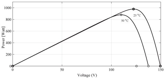
Figure 3.
P–V characteristics of PV array at variable temperature.
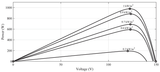
Figure 4.
P–V characteristics of PV array at variable irradiation levels.
The second part of the MPPT stage is DC–DC boost converter which is also shown in Figure 1, where and is the voltage and current generated by the solar array, is the capacitor at the input side of the DC–DC converter that minimizes the ripples in the solar array output voltage. is the inductor and is the current through the inductor. is the duty signal that controls the switching of the IGBT in order to achieve the maximum power. D is the diode, is the capacitor at the output side of the boost converter whereas, is the output voltage of the boost converter taken across output capacitor . By using Kirchhoff’s laws the mathematical model of the boost converter can be written as (7)
By selecting and as state variables, i.e.,
where is control input that controls the switching operation of the boost converter. The input to the boost converter, provided by solar panels, varies with solar radiations, thus, the duty ratio is changed accordingly by the proposed controller in order to track the maximum power point.
3. Integral Back-Stepping Controller Design for DC Stage
The DC stage control strategy has been presented in Figure 5. The reference voltage for the algorithm is generated by the P&O algorithm as presented in [23], and the main objective of the controller design is to track the reference photovoltaic voltage to extract the maximum power from PV panels. Thus, the voltage tracking error is defined as
where and the tracking error derivative can be written as
by inserting the value of from (8) in (10)
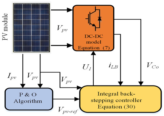
Figure 5.
Boost converter control strategy.
The following Lyapunov function is defined for convergence assurance
the derivative of (12) can be written as
The virtual control command for is which is the desired inductor current for boost converter. In order to achieve error convergence it is necessary to have , thus
where is positive design constant. From (16), the virtual control can be written as
The second error between the second state and its desired value can be defined as
for (18) the can be written as
The second Lyapunov function can be defined as
By inserting (23) and the derivative of (18) in (25)
after rearranging
after inserting the value of from (8)
In order to achieve
Simplifying (29) for duty ratio
is the duty ratio for the boost converter to attain the maximum power from the PV array whereas, and are strictly positive design constants.
4. AC Stage Inverter Modeling
The second stage of the PV system consists of a single-phase DC–AC inverter as shown in Figure 1, where is the input voltage that is supplied by the output of the boost converter, L is the inductor and C is the capacitor that forms the low pass filter whereas are the semiconductor switches that are controlled by the PWM signal generated based on controller output, R describes the linear load whereas, u is the control input. , and are the inductor current, capacitor current and output current, respectively. Output voltage is taken across the filter capacitor which follows the desired sinusoidal reference voltage. Inverter dynamics by using Kirchhoff’s laws are expressed as
For this system, output voltage and inductor current are considered as state variables. In reference tracking, the output voltage is designed in such a way that it is able to track the desired sinusoidal reference even in the presence of linear and non-linear load variations. From (31) it is clear that the load R and DC-state output voltage which serve as input for the second stage, is coupled to the output voltage and inductor current where any variation in the load or input voltage will affect both of the state variables. By considering the direct coupling between and load variation, the system (31) can be re-expressed as follows;
where is the mismatched disturbance that acts on the inverter through the channel that is different from the input channel. is the nominal value of resistance, is assumed to be the only measurable output, i.e., and the control objective is to track a sinusoidal reference voltage such that
5. Super Twisting Controller Design for AC Stage
The disturbance rejection based super twisting sliding mode control strategy has been presented in Figure 6. The main control objective is to develop a robust controller for this VSI system that can track the desired reference sinusoidal voltage with minimized steady-state error and THD in the presence of load variations. In order to proceed with the design, system (32) is transformed where, the first state is defined as
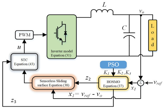
Figure 6.
AC stage control strategy.
By taking derivative of (33) and inserting Equation (32), it becomes
where and . By taking the derivative of (34), it gives
where and thus, the inverter system subjected to load uncertainties can be presented as a class of non-linear dynamic system which contains the system states as a chain of integrals and system uncertainties as a lumped parameter, as follows
where represents the state vector, is the lumped parameter disturbance that includes the so-called matched and mismatched disturbances [41], u is the control input while b is the input matrix. In order to estimate the system states and lumped parameter uncertainty the higher order sliding mode observer for can be defined as
where , and are the observer gains which are designed using particle swarm optimization whereas and are the estimates of and , respectively. The sliding surface can be designed as
where is a positive constant and is the estimate of state that contribute towards observer based sliding surface. By taking the derivative of (8), it gives
By inserting the value of from (6) in (9)
By making the control law (12) can be derived using feedback linearization technique.
where
By inserting the value of b and , then
Normally, in order to achieve fast convergence of sliding variable s, the signum function gains and are designed proportional to the disturbances in the system. However, these high gains result in overlong settling time, overshoot in the sliding variable and chattering in the control input. On the other hand, smaller gain values result in slow convergence. A disturbance estimation and rejection strategy help in implementing the proposed control law with a small controller gain without the loss of robustness. The proposed STC control provides smooth sinusoidal voltage to the PV system load with minimum steady-state error and THD. The stability analysis of the closed loop dynamic STC for the AC stage is presented in the Appendix A.
6. Simulation Results and Discussion
The combined control strategy for the stand-alone PV system is illustrated in Figure 7, which outlines the steps taken to implement the control algorithms for both stages. The hybrid IBSC is implemented for the DC–DC stage and dynamic STC is implemented for the DC–AC stage. The entire strategy is validated through MATLAB Simulink for varying temperature, solar irradiance, and linear and non-linear loads. The performance of the proposed controller is compared with the well established BSC method [23]. The discrete components values used for simulation and designed controller parameters are presented in Table 2, Table 3 and Table 4.
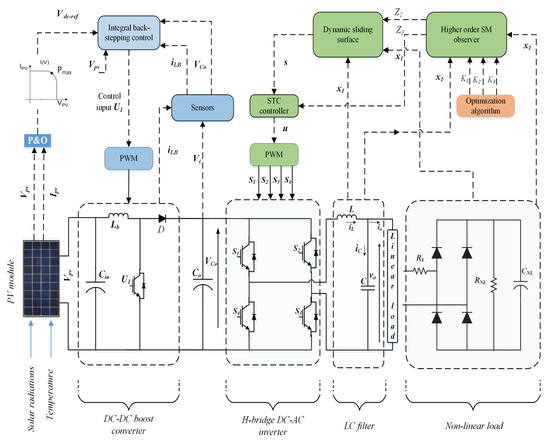
Figure 7.
Combined control strategy.
Table 2.
Simulation parameters for DC stage.
Table 3.
Characteristic values used for simulation for second DC–AC stage.
Table 4.
Super twisting controller parameters for second DC–AC stage.
6.1. Performance Evaluation with Varying Environmental Temperature
At the first stage, the performance is evaluated at a fixed radiation level of 1000 W/m while making a step change in temperature from 25 C to 50 C at a time instant of 0.25 s as shown in Figure 8. Figure 9 shows that both the controller exhibits almost similar responses at room temperature of 25 C however, when a step change in temperature occurs the BSC loses its consistency and oscillations of 18 V amplitude is visible in the PV array output voltage.
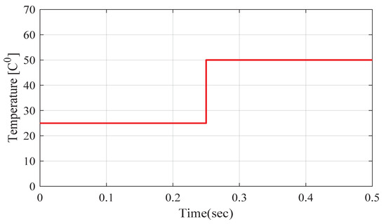
Figure 8.
Temperature variation.
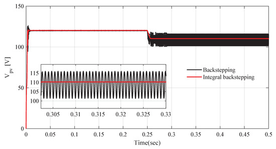
Figure 9.
PV array output voltage.
The similar response in visible in Figure 10 and Figure 11 which depict the maximum power obtained from the PV array and the output voltage of the DC–DC boost converter, respectively.
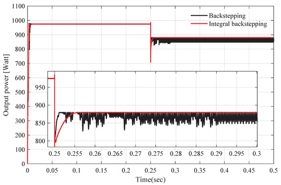
Figure 10.
Maximum power of PV array at variable temperature.
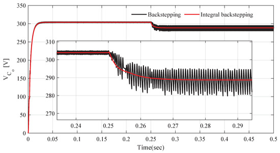
Figure 11.
DC–DC boost converter output at variable temperature.
6.2. Performance Evaluation with Varying Solar Irradiation Level
Figure 12 describes the various solar irradiance levels that are applied to the PV array to examine the dynamic response of the proposed IBSC. The initial value of irradiance is set to 600 W/m; after each 0.2, it is changed to the following values: 200 W/m, 700 W/m, 1000 W/m, and 900 W/m in order to have instantaneous step values of irradiance in a short time for testing the capability of the controller to track the maximum value of power generated by the PV array.
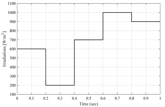
Figure 12.
Variable irradiation pattern.
As the proposed IBSC accumulates the converter output voltage in its design, the integral action mitigates the oscillations in as shown in Figure 13. In addition to the improved response time, there are constant oscillations of almost in the BSC method as compared to the proposed method with nominal oscillations of for the entire irradiation profile.
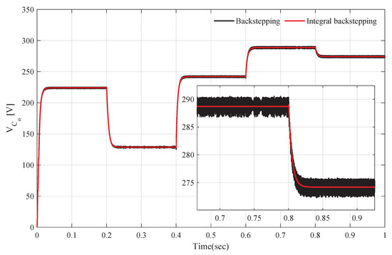
Figure 13.
Boost converter output voltage at variable irradiation profile.
The variation in solar irradiation profile caused significant variation in PV current as presented in Figure 14. The response indicates that the BSC algorithm gives an oscillation of for entire irradiation profile whereas the proposed algorithm gives oscillations of .
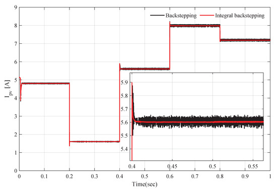
Figure 14.
PV array current.
Both the controllers track the maximum power with accuracy however, there are constant oscillations of for the BSC as compared to for the proposed IBSC as shown in Figure 15, which indicates that the proposed algorithm performs 15 times better than the bench-marked algorithm. The attained values of maximum PV power can be verified from Figure 3 and Figure 4, which indicates that the proposed controller tracks the maximum operating points with accuracy.
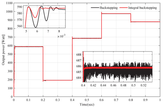
Figure 15.
PV array power at variable irradiation.
Figure 16 presents the efficiency of the DC–DC converter with the proposed IBSC where it gives better efficiency for the entire irradiation profile than its counterpart BSC. The efficiency of the proposed method is almost for the entire irradiation profile except for the time interval between 0.2 and 0.4 s where the efficiency level drops to because of the lowest irradiation level of 200 W/m. Although the 1000 W/m, efficiency is almost , the BSC achieve the maximum efficiency of at this level of irradiation.
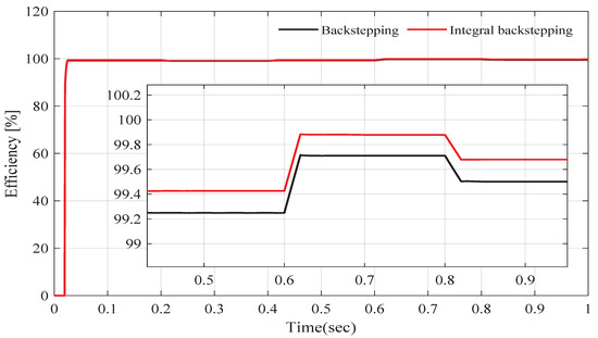
Figure 16.
Efficiency of the DC–DC converter.
6.3. VSI Performance for the Entire Solar Irradiation Profile
The cascaded system reference tracking performance is presented in Figure 17 which shows that the output for the proposed controller approaches steady-state level of 220 V in 0.004 s as the radiation level reaches from 0 to 600 W/m during 0–0.2 s time interval. Correspondingly, the settling time for the BSC during transient interval is around 0.008 s, as shown in Figure 17 and Figure 18.
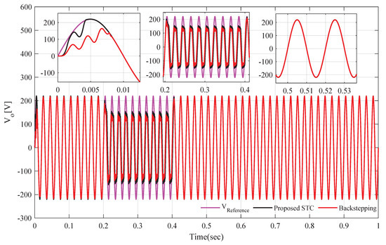
Figure 17.
Reference tracking of cascaded system for entire radiation profile.
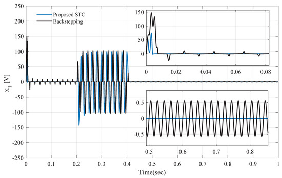
Figure 18.
Tracking error for the entire radiation profile.
Likewise, it is also visible in Figure 17 and Figure 18 that during the transient phase the tracking error for the proposed STC is compared to of the BSC. Meanwhile, when the radiation level drops to 200 W/m there is a tracking error of almost for both the controllers as shown in Figure 18. This high tracking error is because of the practical limitation of control input or duty ratio that cannot be more than . Thus, a saturation limit has been imposed in the simulation setup to keep the duty ratio within the practical limit of as indicated in Figure 19. For the rest of the radiation profile, the inverter output accurately tracks the reference voltage for both of the controllers and the tracking error remains at for STC and for BSC as depicted by Figure 17 and Figure 18, respectively. It is obvious that the inverter output is coupled to the DC–DC converter output voltage which is used to determine the duty ratio level by the expression . Considering the practical limit of duty ratio at 0.9 the inverter gives error-free output long as the remains greater than 244.44 V. It is also clear that the STC control algorithm counteracts the fluctuation of the , as long as its amplitude remains greater than 244.44 V. Thus, for the second stage performance analysis, the rest of the results are presented when the is greater than the threshold level. For that purpose a constant voltage level of 260 V is selected to check the robustness of the disturbance rejection based STC strategy against linear and non-linear loads.
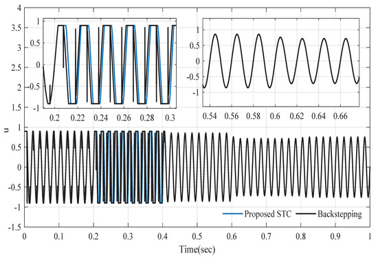
Figure 19.
Control input for the entire radiation profile.
6.4. Case 1: STC Performance Analysis for Linear and Non-Linear Loads
At linear load, both the controllers accurately track the reference voltage and the tracking error immediately converges to zero for the proposed algorithm in contrast to error for the BSC controller, as shown in Figure 20a and Figure 20b, respectively. The load current is quite smooth as depicted in Figure 20c and the estimation errors converge to zero as illustrated in Figure 21 which shows that the designed observer is giving the estimated values correctly. The most common and widely used non-linear load connected to the output of the inverter is full wave bridge rectifier that is used for battery charging purposes, as shown in Figure 1. Under this type of load, the proposed STC exhibits robust reference tracking capability, as shown in Figure 22a. The rectifier current is smooth, and the tracking error converges to zero immediately as presented in Figure 22c and Figure 22b, respectively. In contrast, the BSC controller lacks to follow the reference voltage accurately and gives a steady-state error of , as shown in Figure 22a and Figure 22b, respectively.
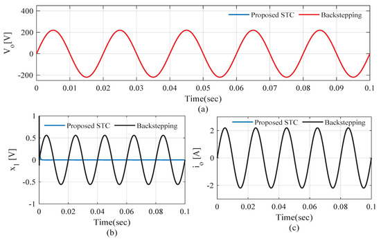
Figure 20.
AC stage performance at constant radiation level for linear load. (a) reference tracking; (b) tracking error; (c) load current.
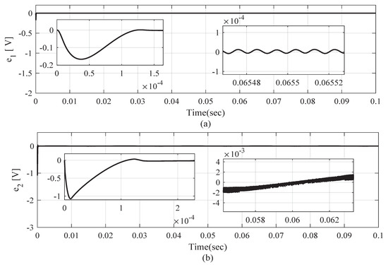
Figure 21.
Observer performance. (a) 1st estimation error; (b) 2nd estimation error.
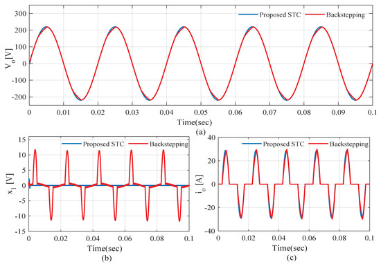
Figure 22.
AC stage performance at constant radiation level for non-linear load. (a) reference tracking; (b) tracking error; (c) load current.
6.5. Case 2: THD Analysis
The proposed HOSMO based STC algorithm exhibit superior performance in terms of harmonic rejection for both linear and non-linear loading conditions. For both types of loads, the THD is limited to and , respectively, for the proposed STC, as illustrated in Figure 23a and Figure 23b, respectively. In parallel, the BSC controller and for the linear and non-linear load as illustrated in Figure 23c and Figure 23d, respectively. Furthermore, a comparison of the proposed algorithm with the previous works is presented in Table 5 which reflects that the proposed controller exhibits superior performance compared to its counterparts.
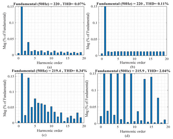
Figure 23.
Total harmonic distortion of the PV system for linear and non-linear load. (a) THD of Proposed control under linear load; (b) THD of Proposed control under non-linear load; (c) THD of backstepping control under linear load; (d) THD of backstepping control under non-linear load.
Table 5.
Proposed SMC and its comparison with other works.
7. Conclusions
In this article, an effective control strategy for a dual-stage single-phase PV system has been presented, where an IBSC has been proposed for the DC stage to extract the maximum available power from the PV array under varying temperature and solar irradiation levels. In contrast, a dynamic STC strategy has been presented to control the operation of VSI, present at the AC stage of the PV system, to attain desired performance under load parameter variations. The effectiveness of the proposed control strategy is evaluated and compared to the BSC in the MATLAB Simulink environment where, the proposed control strategy has shown better performance in terms of response speed, conversion efficiency, reduced steady-state error, and low total harmonic distortion (THD). At the DC stage, the proposed IBSC tracks the MPP effectively with an efficiency of at peak irradiation level compared to of the bench-marked BSC. The results also depict that the designed dynamic STC controller tracks the reference voltage effectively for varying temperature and irradiation levels as long as the remains greater than 244.44 V. The steady-state tracking error remains at 0 V compared to for the BSC whereas the THD remains at and 0.34% for linear and non-linear loads, respectively, as compared to and for the BSC algorithm.
Author Contributions
All the authors contributed significantly. Conceptualization, W.A.; Methodology, W.A. and A.R.H.; Formal analysis, W.A. and H.A.; Supervision, A.R.H. and J.A.A.; Validation, W.A., S.M.F.u.R., and M.P.B.; Visualization, H.A., M.P.B., and S.M.F.u.R.; Writing—Review and editing, W.A. and A.R.H. All authors have read and agreed to the published version of the manuscript.
Funding
The authors received no funding for this project.
Data Availability Statement
Not applicable.
Acknowledgments
We thank the Islamia University of Bahawalpur and the Higher Education Commission of Pakistan for their support. We also thank all the members of Control and Mechatronics Laboratory, Universiti Teknologi Malaysia, for their inputs and sharing.
Conflicts of Interest
The authors declare no conflict of interest.
Appendix A. Stability Analysis
This section illustrates the stability analysis of the proposed closed-loop system in two steps. Firstly, the observer stability is ensured by proving that the error dynamics converge to zero and then it is proved that the sliding surface converge to zero in finite time. For that purpose, the observation errors are defined as
Assumption: the lumped parameter disturbance is bounded and its first order derivative has Lipschitz constant C, i.e., . By taking the derivative of the estimation error (A1) we get the observer error dynamics
For real variable to a real power ,
Consider the following continuous function
The is homogeneous and is differentiable everywhere, but due to the term its is not locally Lipschitz [43]. There exist a condition for the coefficients and gains of the observer, such that and . The is in quadratic form for the vector
will be positive definite if and only if . To prove positive definite the mode of is given as,
The is positive definite and radially unbounded if, and only if,
given in (A11) will be negative definite, i.e., for every value of lumped disturbance if
Thus, the error dynamics presented in (A3) will converge to zero in finite time. After the error convergence observer’s , and in Equation (37) approach to , and in finite time.
Sliding Surface Convergence
Stability of proposed control law is proved using Lyapunov stability criteria. Let us consider a positive definite Lyapunov candidate
by inserting the value of from (39)
by substituting the value of from (36)
By substituting the value of u(t)
Which then reduces to the following form
By the virtue of observer convergence is bounded and significantly small which leaves
where thus result in, any positive value for and will will result
this completes the proof.
References
- Andrychowicz, M. Optimization of distribution systems by using RES allocation and grid development. In Proceedings of the 2018 15th International Conference on the European Energy Market (EEM), Lodz, Poland, 27–29 June 2018. [Google Scholar] [CrossRef]
- Ahmed, M.; Abdelrahem, M.; Kennel, R. Highly efficient and robust grid connected photovoltaic system based model predictive control with Kalman filtering capability. Sustainability 2020, 12, 4542. [Google Scholar] [CrossRef]
- Bollipo, R.B.; Mikkili, S.; Bonthagorla, P.K. Critical Review on PV MPPT Techniques: Classical, Intelligent and Optimisation. IET Renew. Power Gener. 2020, 14, 1433–1452. [Google Scholar] [CrossRef]
- Alam, A.; Verma, P.; Tariq, M.; Sarwar, A.; Alamri, B.; Zahra, N.; Urooj, S. Jellyfish search optimization algorithm for mpp tracking of pv system. Sustainability 2021, 13, 1736. [Google Scholar] [CrossRef]
- Fei, J.; Zhu, Y. Adaptive fuzzy sliding control of single-phase PV grid-connected inverter. PLoS ONE 2017, 12, e0182916. [Google Scholar] [CrossRef] [Green Version]
- Andrychowicz, M. Res and es integration in combination with distribution grid development using milp. Energies 2021, 14, 383. [Google Scholar] [CrossRef]
- Chaibi, Y.; Salhi, M.; El-Jouni, A. Sliding mode controllers for standalone PV systems: Modeling and approach of control. Int. J. Photoenergy 2019, 2019, 5092078. [Google Scholar] [CrossRef] [Green Version]
- Iftikhar, R.; Ahmad, I.; Arsalan, M.; Naz, N.; Ali, N.; Armghan, H. MPPT for photovoltaic system using nonlinear controller. Int. J. Photoenergy 2018, 2018, 6979723. [Google Scholar] [CrossRef] [Green Version]
- Femia, N.; Petrone, G.; Spagnuolo, G.; Vitelli, M. Optimization of perturb and observe maximum power point tracking method. IEEE Trans. Power Electron. 2005, 20, 963–973. [Google Scholar] [CrossRef]
- Faraji, R.; Rouholamini, A.; Naji, H.R.; Fadaeinedjad, R.; Chavoshian, M.R. FPGA-based real time incremental conductance maximum power point tracking controller for photovoltaic systems. IET Power Electron. 2014, 7, 1294–1304. [Google Scholar] [CrossRef]
- Fang, Y.; Zhu, Y.; Fei, J. Adaptive intelligent sliding mode control of a photovoltaic grid-connected inverter. Appl. Sci. 2018, 8, 1756. [Google Scholar] [CrossRef] [Green Version]
- De Brito, M.A.G.; Galotto, L.; Sampaio, L.P.; De Azevedo Melo, G.; Canesin, C.A. Evaluation of the main MPPT techniques for photovoltaic applications. IEEE Trans. Ind. Electron. 2013, 60, 1156–1167. [Google Scholar] [CrossRef]
- Mostafa, M.R.; Saad, N.H.; El-sattar, A.A. Tracking the maximum power point of PV array by sliding mode control method. Ain Shams Eng. J. 2020, 11, 119–131. [Google Scholar] [CrossRef]
- Na, W.; Chen, P.; Kim, J. An improvement of a fuzzy logic-controlled maximum power point tracking algorithm for photovoltic applications. Appl. Sci. 2017, 7, 326. [Google Scholar] [CrossRef]
- Elobaid, L.M.; Abdelsalam, A.K.; Zakzouk, E.E. Artificial neural network-based photovoltaic maximum power point tracking techniques: A survey. IET Renew. Power Gener. 2015, 9, 1043–1063. [Google Scholar] [CrossRef]
- Kalibatien, D.; Miliauskait, J. A Hybrid Systematic Review Approach on Complexity Issues in Data-Driven Fuzzy Inference Systems Development. Informatica 2021, 32, 85–118. [Google Scholar] [CrossRef]
- Ben Smida, M.; Sakly, A. Genetic based algorithm for maximum power point tracking (MPPT) for grid connected PV systems operating under partial shaded conditions. In Proceedings of the 7th International Conference on Modelling, Identification and Control (ICMIC) 2015, Sousse, Tunisia, 18–20 December 2015. [Google Scholar] [CrossRef]
- Mohanty, S.; Subudhi, B.; Ray, P.K. A new MPPT design using grey Wolf optimization technique for photovoltaic system under partial shading conditions. IEEE Trans. Sustain. Energy 2016, 7, 181–188. [Google Scholar] [CrossRef]
- Sundareswaran, K.; Vigneshkumar, V.; Sankar, P.; Simon, S.P.; Srinivasa Rao Nayak, P.; Palani, S. Development of an Improved P&O Algorithm Assisted Through a Colony of Foraging Ants for MPPT in PV System. IEEE Trans. Ind. Inform. 2016, 12, 187–200. [Google Scholar] [CrossRef]
- Eltamaly, A.M.; Al-Saud, M.S.; Abo-Khalil, A.G. Performance improvement of PV systems’ maximum power point tracker based on a scanning PSO particle strategy. Sustainability 2020, 12, 1185. [Google Scholar] [CrossRef] [Green Version]
- Eltamaly, A.M. A novel musical chairs algorithm applied for MPPT of PV systems. Renew. Sustain. Energy Rev. 2021, 146, 111135. [Google Scholar] [CrossRef]
- Ali, H.G.; Arbos, R.V.; Herrera, J.; Tobón, A.; Peláez-Restrepo, J. Non-linear sliding mode controller for photovoltaic panels with maximum power point tracking. Processes 2020, 8, 108. [Google Scholar] [CrossRef] [Green Version]
- Diouri, O.; Es-Sbai, N.; Errahimi, F.; Gaga, A.; Alaoui, C. Modeling and Design of Single-Phase PV Inverter with MPPT Algorithm Applied to the Boost Converter Using Back-Stepping Control in Standalone Mode. Int. J. Photoenergy 2019, 2019, 7021578. [Google Scholar] [CrossRef]
- Ajangnay, M.O.; Alsokhiry, F.; Adam, G.P.; Alabdulwahab, A. Back-stepping Control of Off-Grid PV Inverter. In Proceedings of the 9th International Conference on Renewable Energy Research and Applications, ICRERA 2020, Glasgow, UK, 27–30 September 2020; pp. 384–389. [Google Scholar]
- Huang, J.; Xu, D.; Yan, W.; Ge, L.; Yuan, X. Nonlinear Control of Back-to-Back VSC-HVDC System via Command-Filter Backstepping. J. Control Sci. Eng. 2017, 2017, 7410392. [Google Scholar] [CrossRef]
- Xu, D.; Dai, Y.; Yang, C.; Yan, X. Adaptive fuzzy sliding mode command-filtered backstepping control for islanded PV microgrid with energy storage system. J. Frankl. Inst. 2019, 356, 1880–1898. [Google Scholar] [CrossRef]
- El Malah, M.; Ba-Razzouk, A.; Abdelmounim, E.; Madark, M. Integral backstepping based nonlinear control for maximum power point tracking and unity power factor of a grid connected hybrid wind-photovoltaic system. Indones. J. Electr. Eng. Inform. 2020, 8, 706–722. [Google Scholar] [CrossRef]
- Ali, K.; Khan, Q.; Ullah, S.; Khan, I.; Khan, L. Nonlinear robust integral backstepping based MPPT control for stand-alone photovoltaic system. PLoS ONE 2020, 15, e0231749. [Google Scholar] [CrossRef]
- Ozdemir, A.; Yazici, I.; Erdem, Z. Model-reference sliding mode control of a three-phase four-leg voltage source inverter for stand-alone distributed generation systems. Turk. J. Electr. Eng. Comput. Sci. 2015, 23, 1817–1833. [Google Scholar] [CrossRef] [Green Version]
- Kumar, N.; Saha, T.K.; Dey, J. Sliding mode control, implementation and performance analysis of standalone PV fed dual inverter. Sol. Energy 2017, 155, 1178–1187. [Google Scholar] [CrossRef]
- Wang, Z.; Li, S.; Yang, J.; Li, Q. Current sensorless sliding mode control for direct current-alternating current inverter with load variations via a USDO approach. IET Power Electron. 2018, 11, 1389–1398. [Google Scholar] [CrossRef]
- Benchouia, M.T.; Ghadbane, I.; Golea, A.; Srairi, K.; Benbouzid, M.H. Design and implementation of sliding mode and PI controllers based control for three phase shunt active power filter. Energy Procedia 2014, 50, 504–511. [Google Scholar] [CrossRef] [Green Version]
- Li, Z.; Member, S.; Zang, C.; Zeng, P.; Yu, H. Control of A Grid-Forming Inverter Based on Sliding Mode and Mixed H 2 /H-infinity Control. IEEE Trans. Ind. Electron. 2017, 64, 3862–3872. [Google Scholar] [CrossRef]
- Pichan, M.; Rastegar, H. Sliding-mode control of four-leg inverter with fixed switching frequency for uninterruptible power supply applications. IEEE Trans. Ind. Electron. 2017, 64, 6805–6814. [Google Scholar] [CrossRef]
- Lauria, D.; Coppola, M. Design and control of an advanced PV inverter. Sol. Energy 2014, 110, 533–542. [Google Scholar] [CrossRef]
- Kamal, S.; Moreno, J.A.; Chalanga, A.; Bandyopadhyay, B.; Fridman, L.M. Continuous terminal sliding-mode controller. Automatica 2016, 69, 308–314. [Google Scholar] [CrossRef]
- Guo, B.; Su, M.; Sun, Y.; Wang, H.; Dan, H.; Tang, Z.; Cheng, B. A Robust Second-Order Sliding Mode Control for Single-Phase Photovoltaic Grid-Connected Voltage Source Inverter. IEEE Access 2019, 7, 53202–53212. [Google Scholar] [CrossRef]
- Pizzo, A.D.; Noia, L.P.D.; Meo, S. Super Twisting Sliding Mode control of Smart inverters grid- connected for PV Applications. In Proceedings of the 6th International Conference on Renewable Energy Research and Applications, San Diego, CA, USA, 5–8 November 2017; Volume 5, pp. 793–796. [Google Scholar]
- Fei, J.; Zhu, Y.; Hua, M. Disturbance observer based fuzzy sliding mode control of PV grid connected inverter. IEEE Access 2018, 6, 18–22. [Google Scholar] [CrossRef]
- Zhu, Y.; Fei, J. Adaptive Global Fast Terminal Sliding Mode Control of Gridconnected Photovoltaic System Using Fuzzy Neural Network Approach. IEEE Access 2017, 5, 109–112. [Google Scholar]
- Wang, C.; Ohsumi, A.; Djurovic, I. Model Predictive Control of Quasi-Z-Source Four-Leg Inverter. IEEE Trans. Ind. Electron. 2016, 63, 1404–1407. [Google Scholar] [CrossRef]
- Komurcugil, H.; Altin, N.; Ozdemir, S.; Sefa, I. An extended lyapunov-function-based control strategy for single-phase UPS inverters. IEEE Trans. Power Electron. 2015, 30, 3976–3983. [Google Scholar] [CrossRef]
- Moreno, J.A. Lyapunov function for Levant’s Second Order Differentiator. Proc. IEEE Conf. Decis. Control 2012, 2, 6448–6453. [Google Scholar] [CrossRef]
Publisher’s Note: MDPI stays neutral with regard to jurisdictional claims in published maps and institutional affiliations. |
© 2022 by the authors. Licensee MDPI, Basel, Switzerland. This article is an open access article distributed under the terms and conditions of the Creative Commons Attribution (CC BY) license (https://creativecommons.org/licenses/by/4.0/).