
A Hybrid Vegetation Detection Framework: Integrating Vegetation Indices and Convolutional Neural Network


 ,
,  , , , and
Abstract
:1. Introduction
2. Background
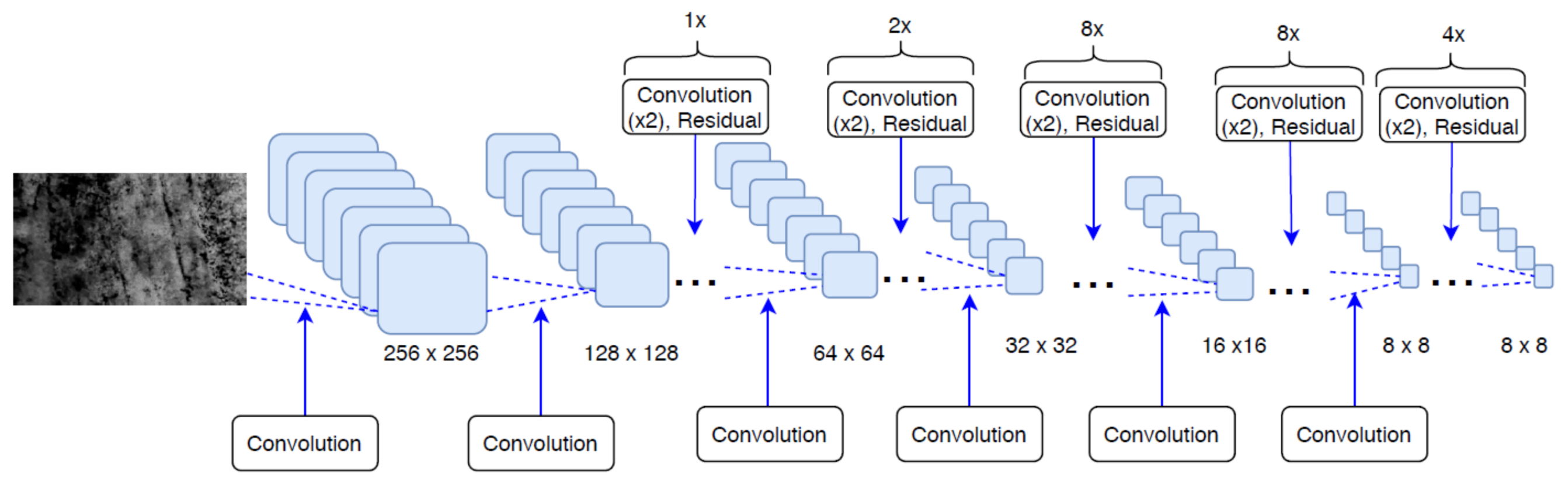
2.1. You Only Look Once (YOLO)
2.2. Vegetation Indices
2.2.1. Green Leaf Index (GLI)
2.2.2. Vegetation Indices Green (VIgreen)
2.2.3. Visible Atmospheric Resistant Index (VARI)
3. Related Studies
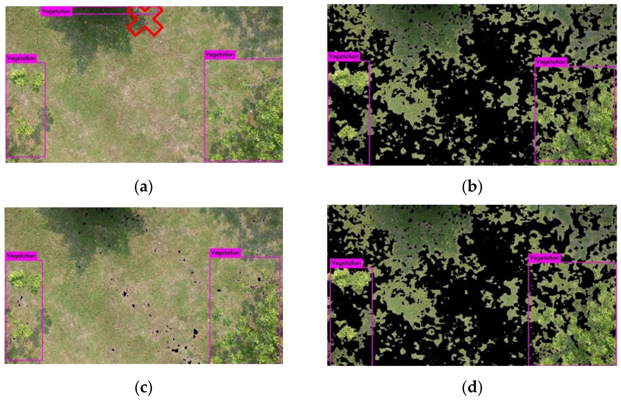
4. Method
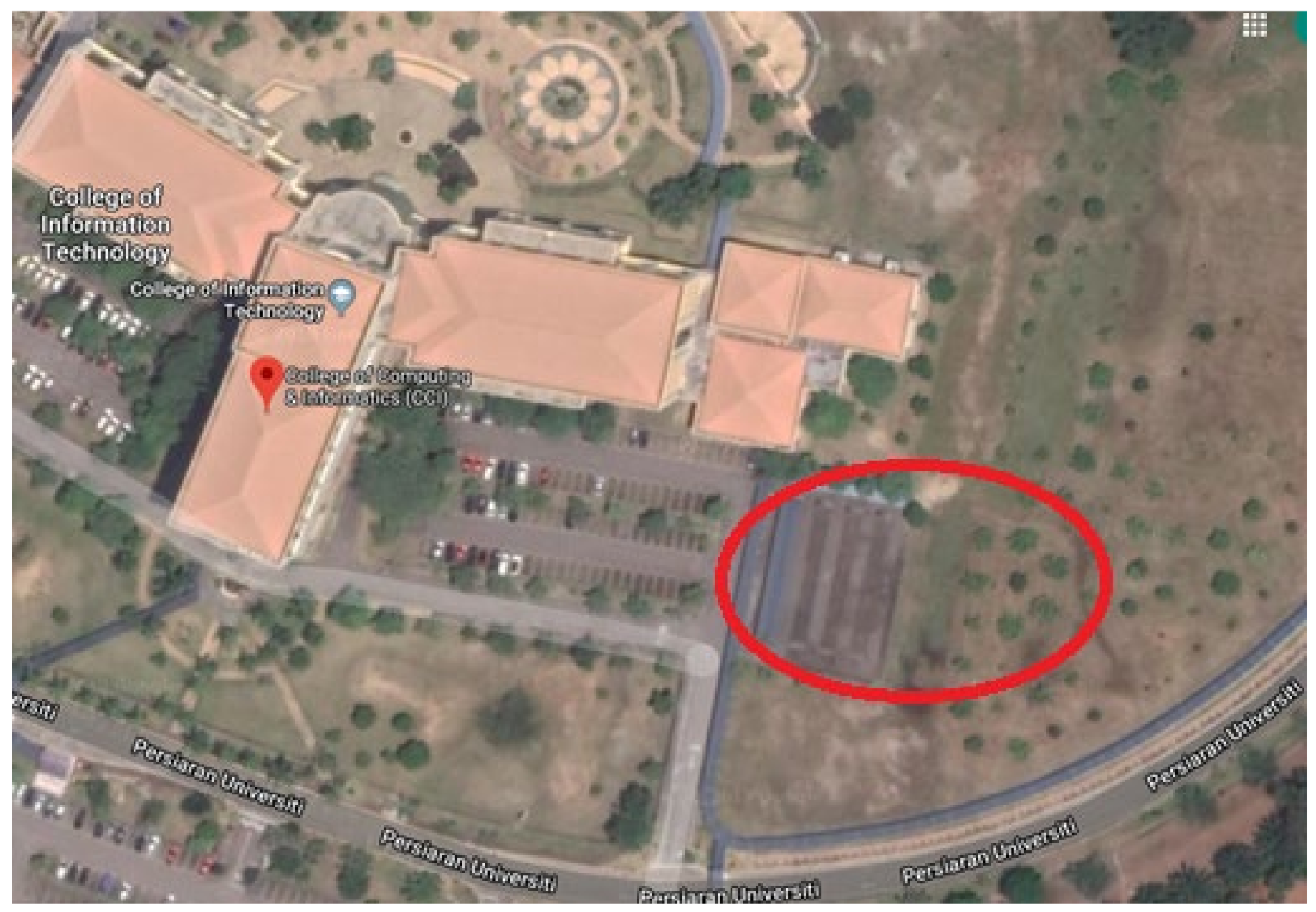
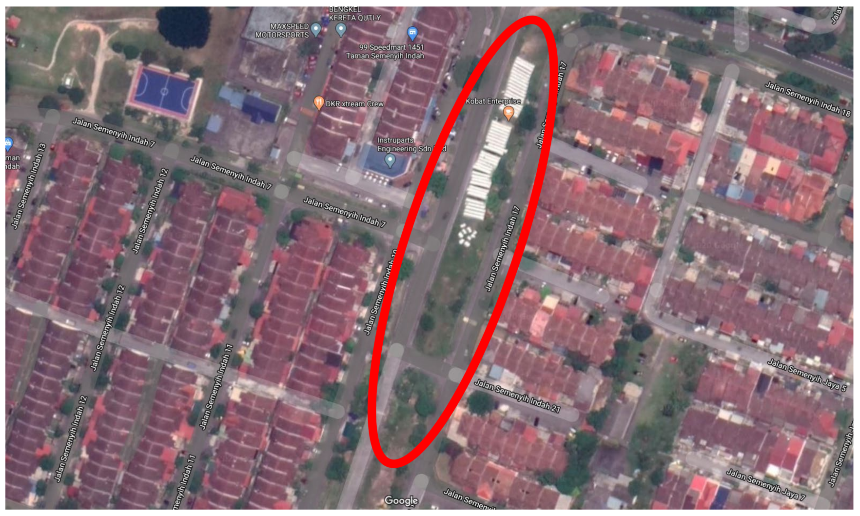
4.1. Data Collection
4.2. Dataset
4.3. Data Processing
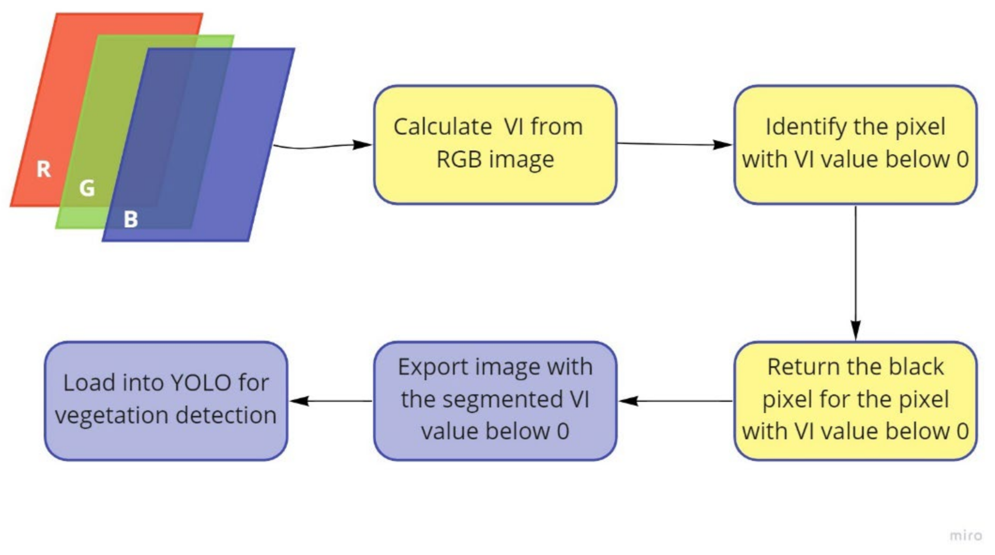
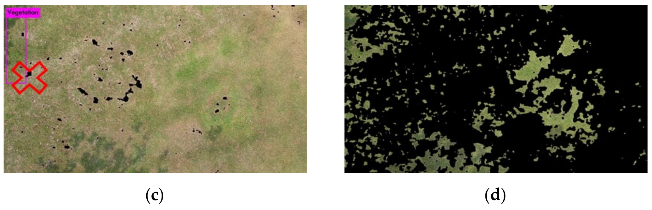
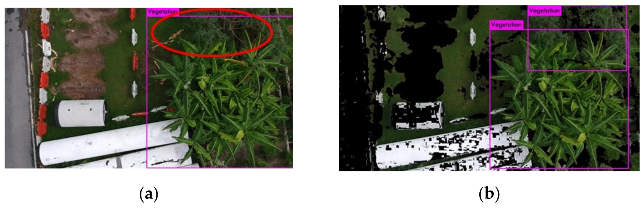
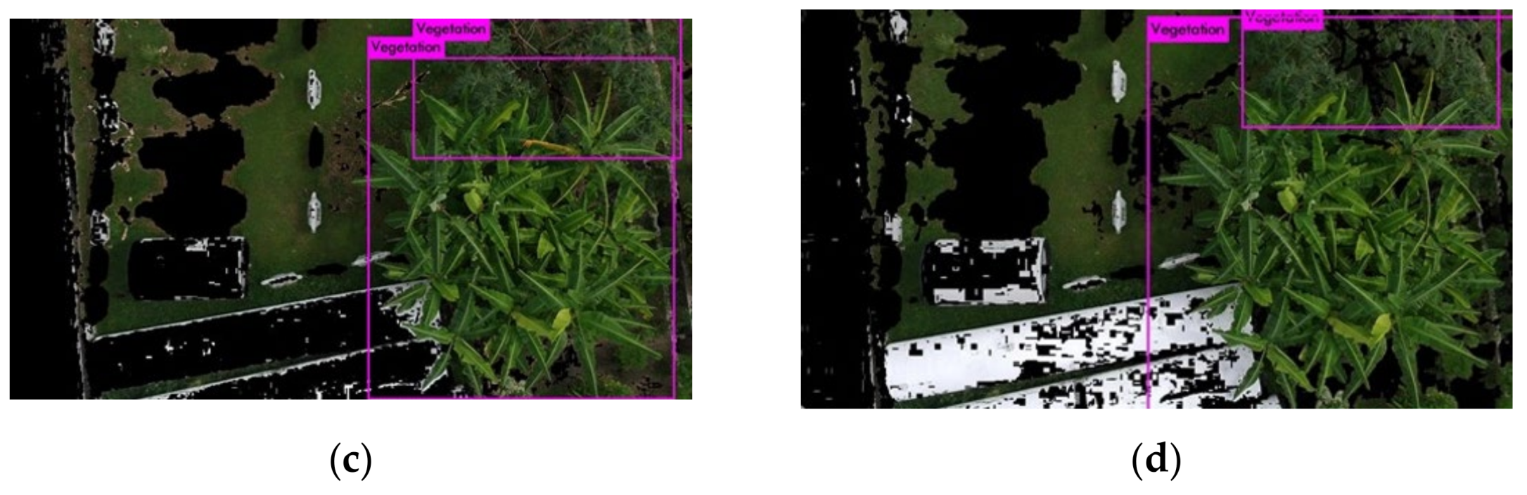
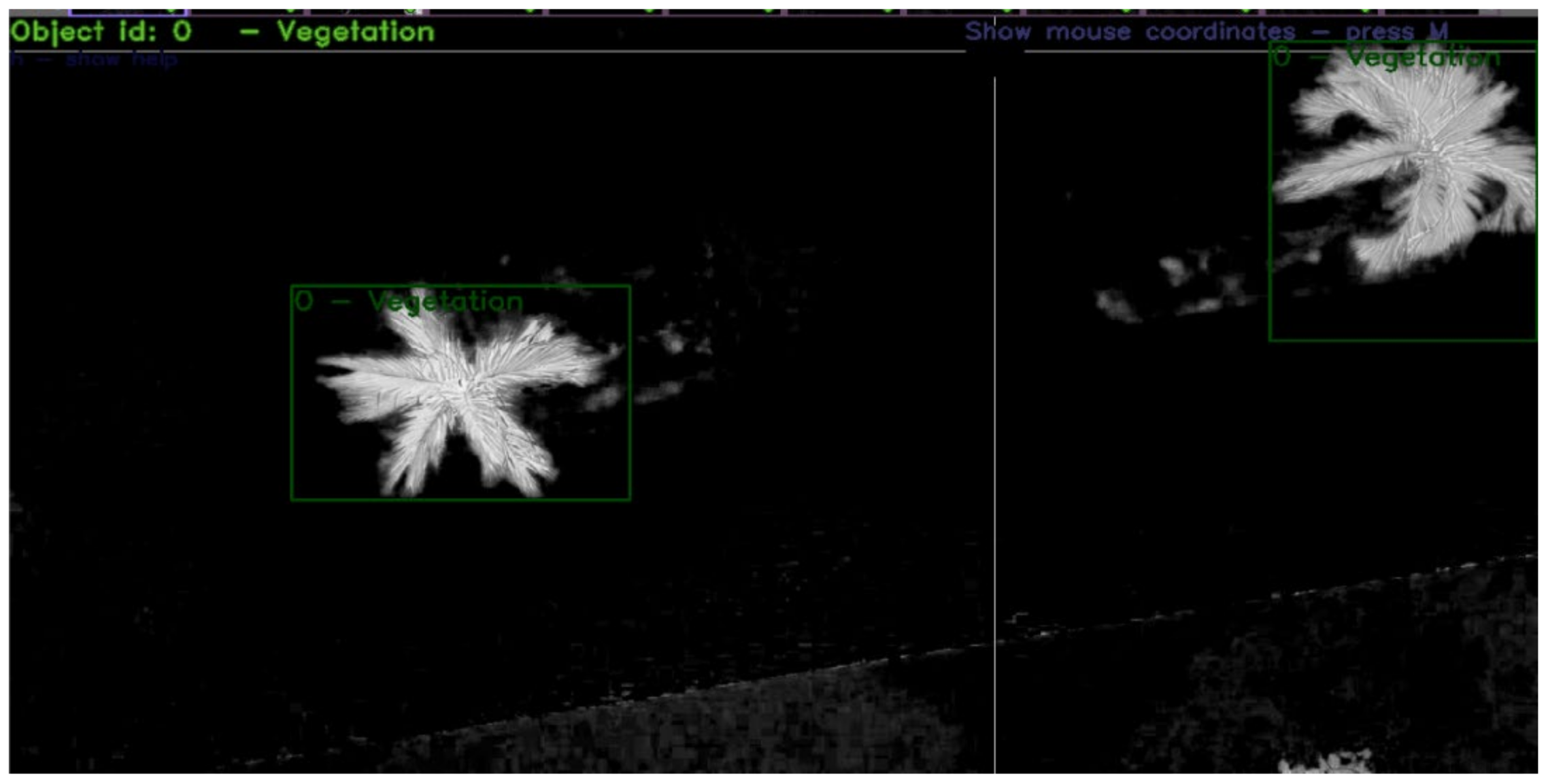
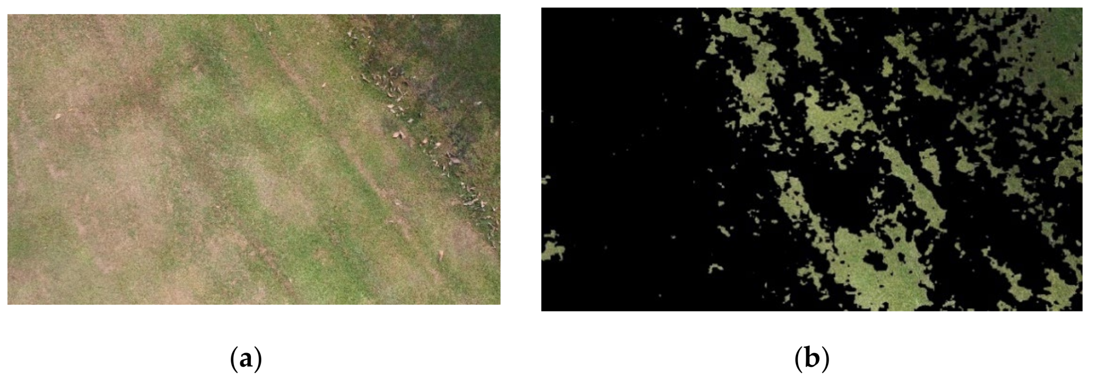
4.4. Image Processing
4.5. Training
4.6. Analysis
5. Results
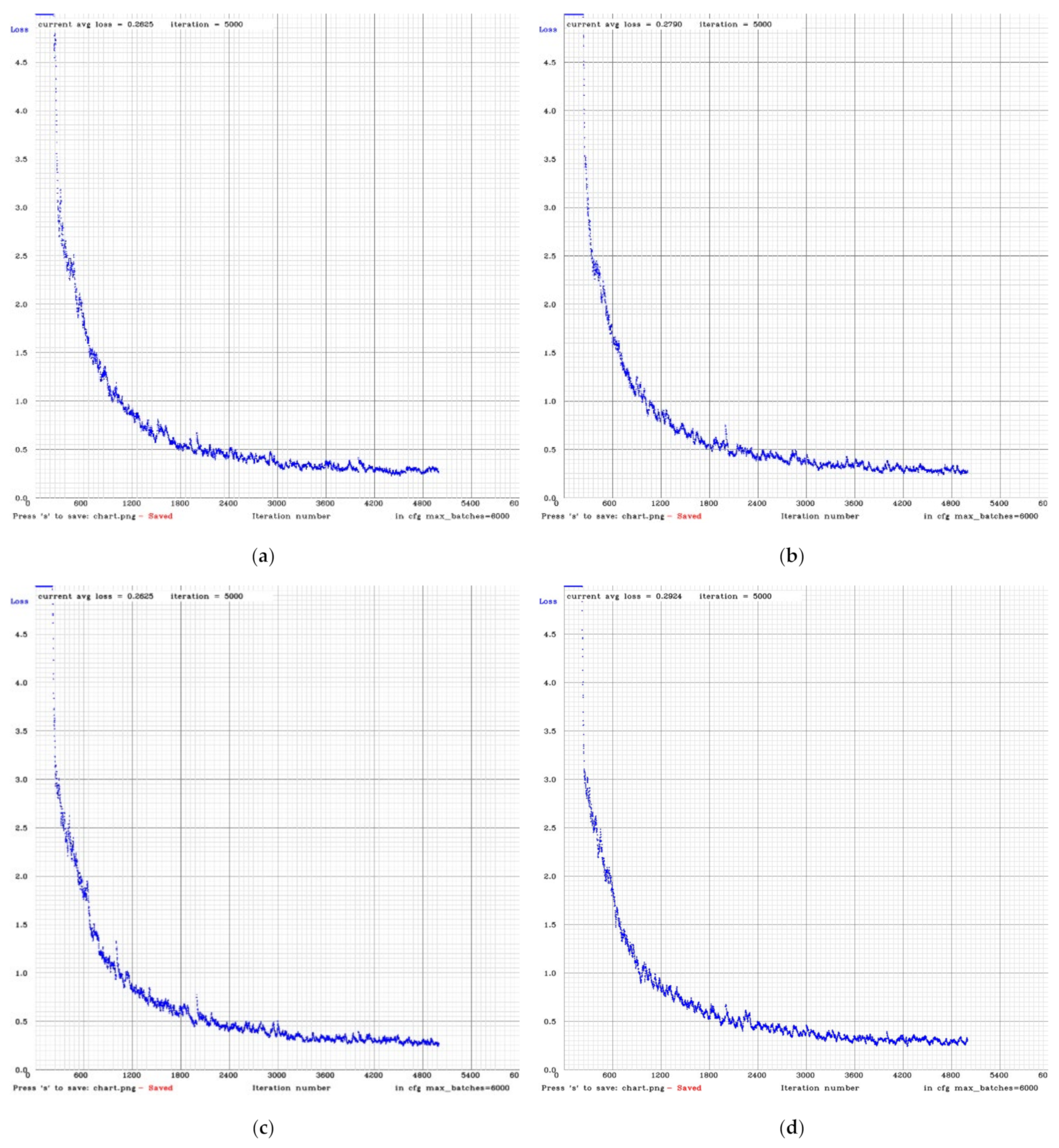
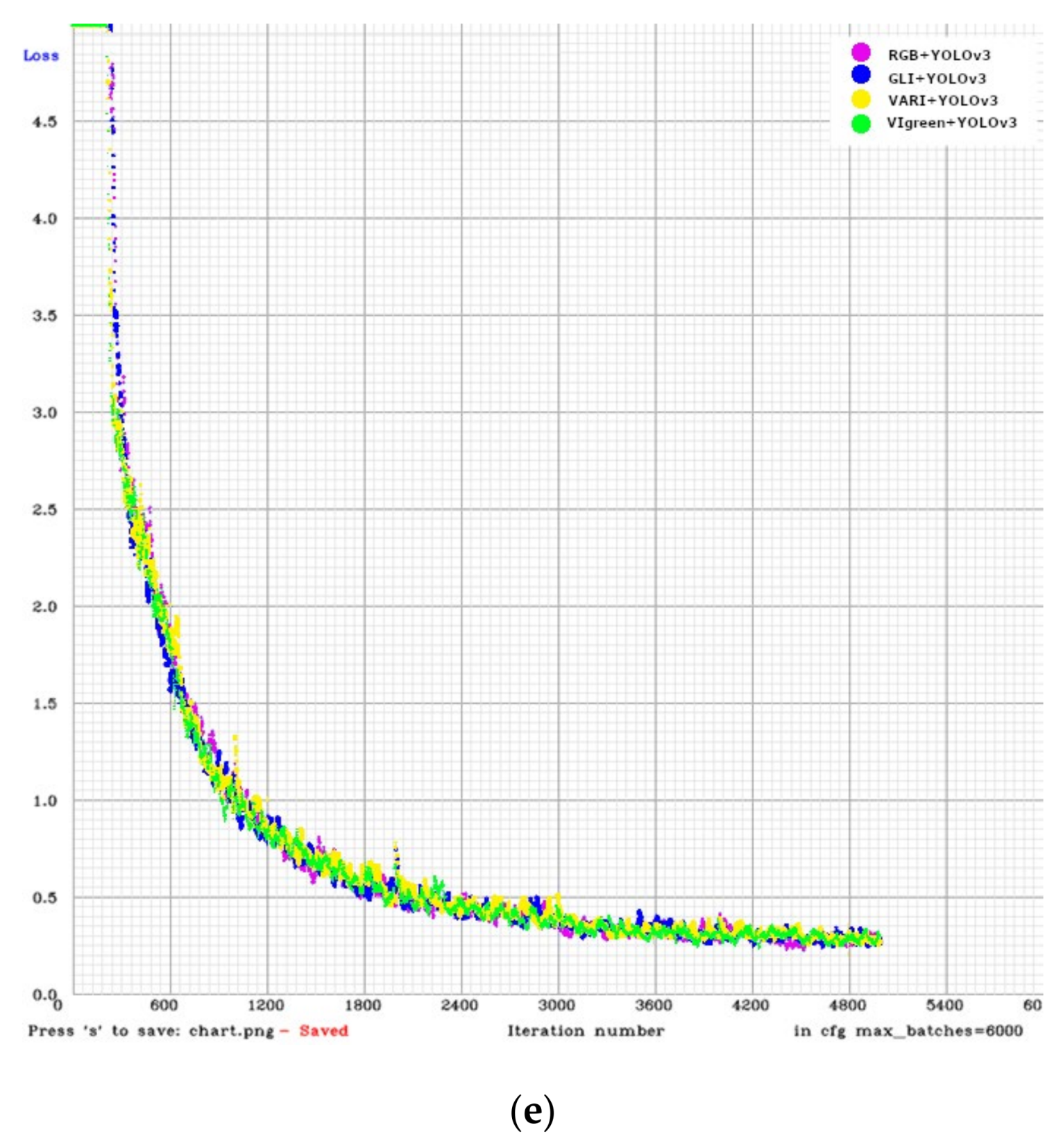
5.1. Convergence Graph Comparison
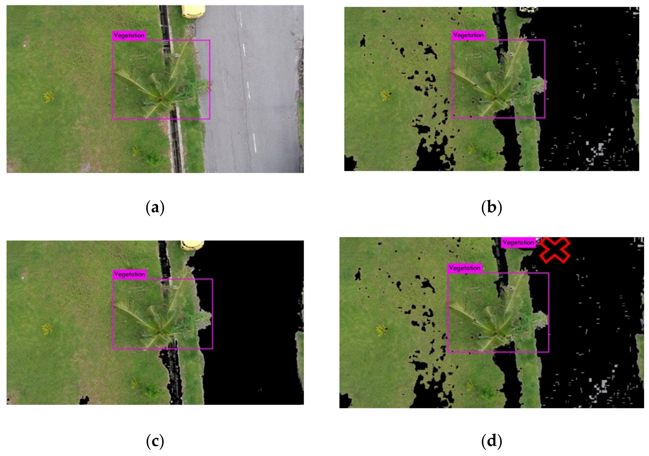
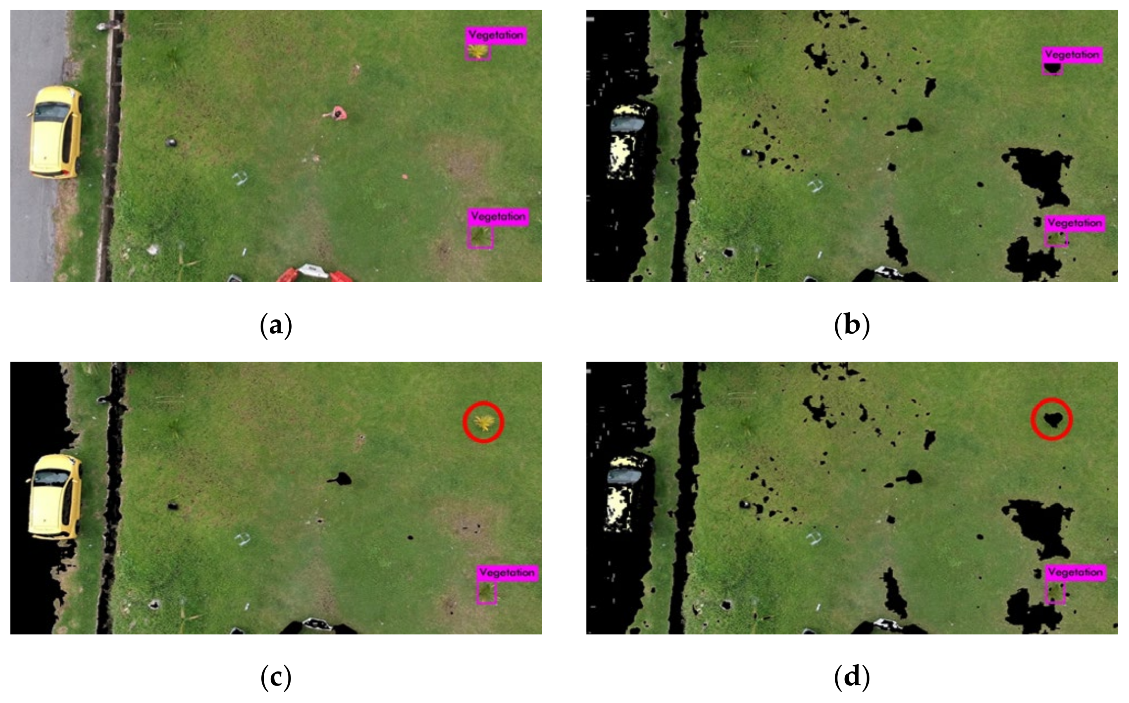
5.2. Confusion Matrix Analysis
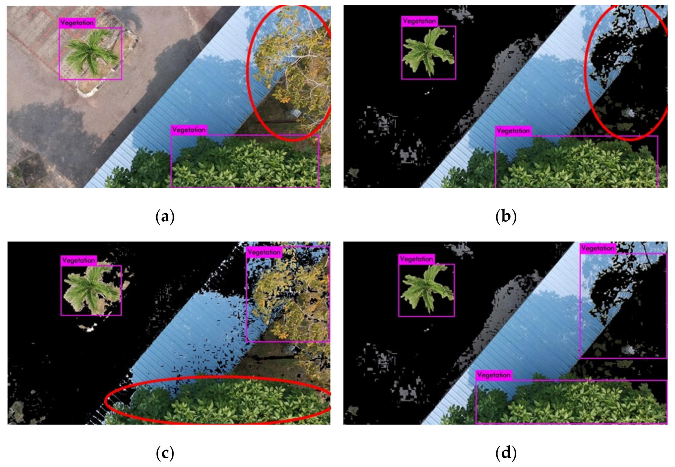
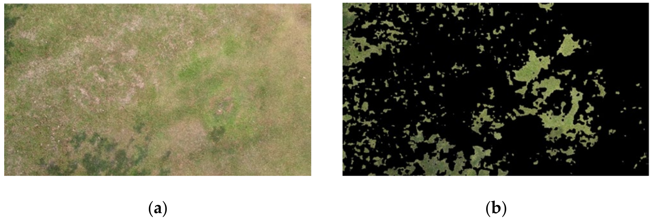
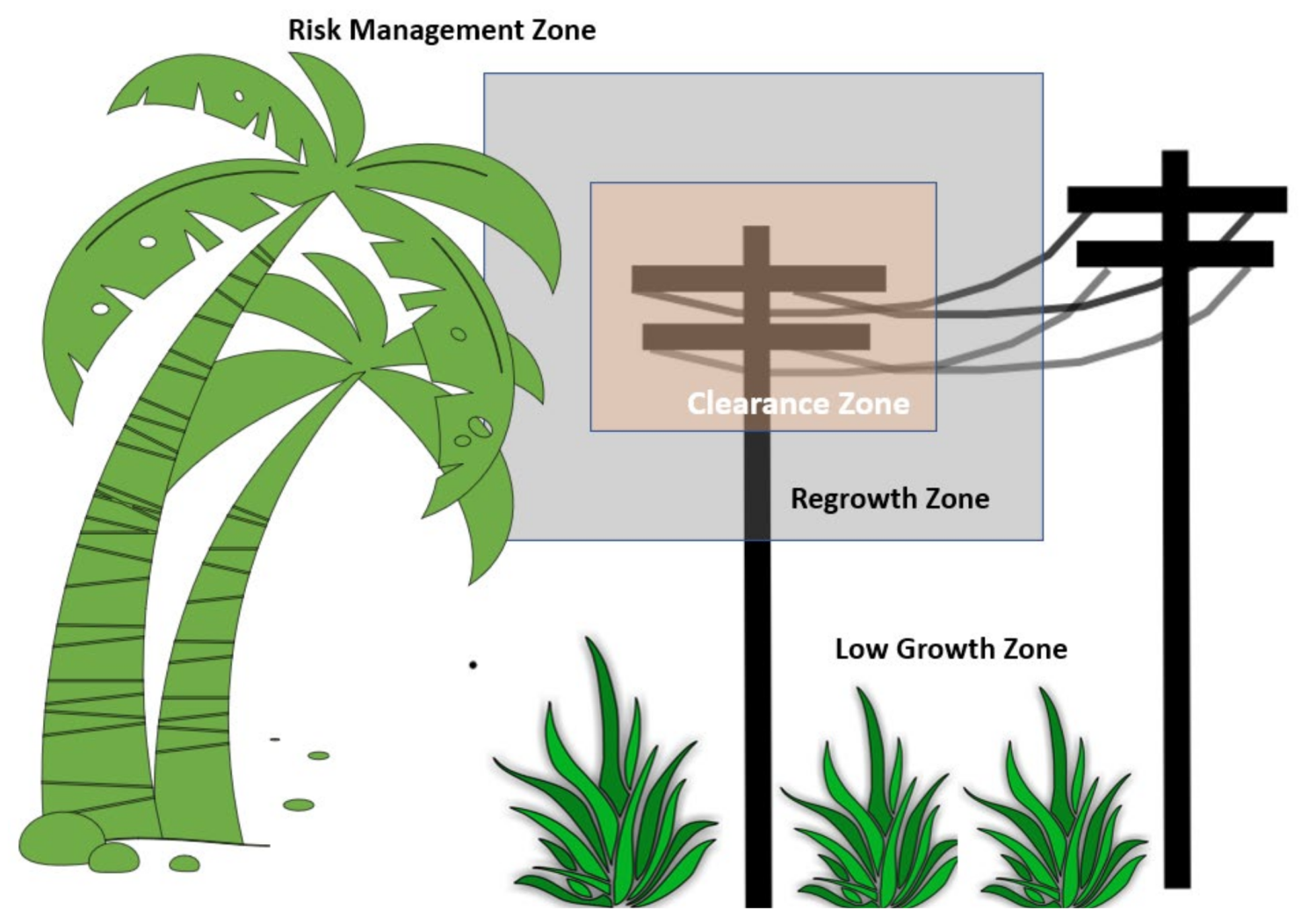
6. Discussion
7. Implications
8. Future Work
9. Conclusions
Author Contributions
Funding
Data Availability Statement
Acknowledgments
Conflicts of Interest
References
- Li, Z.; Walker, R.; Hayward, R.; Mejias, L. Advances in Vegetation Management for Power Line Corridor Monitoring Using Aerial Remote Sensing Techniques. In Proceedings of the 2010 1st International Conference on Applied Robotics for the Power Industry, Montreal, QC, Canada, 5–7 October 2010; pp. 1–6. [Google Scholar]
- Kalapala, M. Estimation of Tree Count from Satellite Imagery through Mathematical Morphology. Int. J. Adv. Res. Comput. Sci. Softw. Eng. 2014, 4, 490–495. [Google Scholar]
- Berni, J.A.J.; Zarco-Tejada, P.J.; Suárez, L.; González-Dugo, V.; Fereres, E. Remote Sensing of Vegetation From UAV Platforms Using Lightweight Multispectral and Thermal Imaging Sensors. Int. Arch. Photogramm. Remote Sens. Spat. Inform. Sci. 2009, 38, 6. [Google Scholar]
- Feng, Q.; Liu, J.; Gong, J. UAV Remote sensing for urban vegetation mapping using random forest and texture analysis. Remote Sens. 2015, 7, 1074–1094. [Google Scholar] [CrossRef] [Green Version]
- Kaneko, K.; Nohara, S. Review of Effective Vegetation Mapping Using the UAV (Unmanned Aerial Vehicle) Method. J. Geogr. Inf. Syst. 2014, 6, 733–742. [Google Scholar] [CrossRef] [Green Version]
- Watanabe, Y.; Kawahara, Y. UAV Photogrammetry for Monitoring Changes in River Topography and Vegetation. Procedia Eng. 2016, 154, 317–325. [Google Scholar] [CrossRef] [Green Version]
- Xue, J.; Su, B. Significant Remote Sensing Vegetation Indices: A Review of Developments and Applications. J. Sens. 2017, 2017, 1353691. [Google Scholar] [CrossRef] [Green Version]
- Gitelson, A.A.; Kaufman, Y.J.; Stark, R.; Rundquist, D. Novel algorithms for remote estimation of vegetation fraction. Remote Sens. Environ. 2002, 80, 76–87. [Google Scholar] [CrossRef] [Green Version]
- Louhaichi, M.; Borman, M.M.; Johnson, D.E. Spatially Located Platform and Aerial Photography for Documentation of Grazing Impacts on Wheat. Geocarto Int. 2001, 16, 65–70. [Google Scholar] [CrossRef]
- Harbaš, I.; Prentašić, P.; Subašić, M. Detection of roadside vegetation using Fully Convolutional Networks. Image Vis. Comput. 2018, 74, 1–9. [Google Scholar] [CrossRef]
- Li, L. The UAV intelligent inspection of transmission lines. In Proceedings of the 2015 International Conference on Advances in Mechanical Engineering and Industrial Informatics, Zhengzhou, China, 11–12 April 2015. [Google Scholar]
- Gopinath, G. Free data and Open Source Concept for Near Real Time Monitoring of Vegetation Health of Northern Kerala, India. Aquat. Procedia 2015, 4, 1461–1468. [Google Scholar] [CrossRef]
- Modzelewska, A.; Stereńczak, K.; Mierczyk, M.; Maciuk, S.; Bałazy, R.; Zawiła-Niedźwiecki, T. Sensitivity of vegetation indices in relation to parameters of Norway spruce stands. Folia For. Pol. Ser. A 2017, 59, 85–98. [Google Scholar] [CrossRef] [Green Version]
- Dustin, M.C. Monitoring Parks with Inexpensive UAVS: Cost Benefits Analysis for Monitoring and Maintaining Parks Facilities; University of Southern California: Los Angeles, CA, USA, 2015. [Google Scholar]
- Xiao, C.; Qin, R.; Huang, X. Treetop detection using convolutional neural networks trained through automatically generated pseudo labels. Int. J. Remote Sens. 2020, 41, 3010–3030. [Google Scholar] [CrossRef]
- Di Leo, E. Individual Tree Crown detection in UAV remote sensed rainforest RGB images through Mathematical Morphology. Remote Sens. 2019, 11, 1309. [Google Scholar]
- Mckinnon, T.; Hoff, P. Comparing RGB-Based Vegetation Indices with NDVI for Drone Based Agricultural Sensing. Agribotix. Com. 2017, 21, 1–8. [Google Scholar]
- Redmon, J.; Farhadi, A. YOLOv3: An Incremental Improvement. arXiv 2018, arXiv:1804.02767. [Google Scholar]
- Grivina, Y.; Andri, S.; Abdi, S. Analisis Pengunaan Saluran Visible Untuk Estimasi Kandungan Klorofil Daun Pade Dengan Citra Hymap. (Studi Kasus: Kabupaten Karawang, Jawa Barat). J. Geod. Undip. 2016, 5, 200–207. [Google Scholar]
- Barbosa, B.D.; Ferraz, G.A.; Gonçalves, L.M.; Marin, D.B.; Maciel, D.T.; Ferraz, P.F.; Rossi, G. RGB vegetation indices applied to grass monitoring: A qualitative analysis. Agron. Res. 2019, 17, 349–357. [Google Scholar]
- Tucker, C.J. Red and photographic infrared linear combinations for monitoring vegetation. Remote Sens. Environ. 1979, 8, 127. [Google Scholar] [CrossRef] [Green Version]
- Bassine, F.Z.; Errami, A.; Khaldoun, M. Vegetation Recognition Based on UAV Image Color Index. In Proceedings of the 2019 IEEE International Conference on Environment and Electrical Engineering and 2019 IEEE Industrial and Commercial Power Systems Europe, Genova, Italy, 10–14 June 2019; pp. 1–4. [Google Scholar]
- Motohka, T.; Nasahara, K.N.; Oguma, H.; Tsuchida, S. Applicability of Green-Red Vegetation Index for Remote Sensing of Vegetation Phenology. Remote Sens. 2010, 2, 2369–2387. [Google Scholar] [CrossRef] [Green Version]
- Sanseechan, P.; Saengprachathanarug, K.; Posom, J.; Wongpichet, S.; Chea, C.; Wongphati, M. Use of vegetation indices in monitoring sugarcane white leaf disease symptoms in sugarcane field using multispectral UAV aerial imagery. IOP Conf. Ser. Earth Environ. Sci. 2019, 301, 012025. [Google Scholar] [CrossRef]
- Mokarram, M.; Hojjati, M.; Roshan, G.; Negahban, S. Modeling The Behavior of Vegetation Indices in the Salt Dome of Korsia in North-East of Darab, Fars, Iran. Model. Earth Syst. Environ. 2015, 1, 27. [Google Scholar] [CrossRef] [Green Version]
- Mokarram, M.; Boloorani, A.D.; Hojati, M. Relationship Between Land Cover And Vegetation Indices. Case Study: Eghlid Plain, Fars Province, Iran. Eur. J. Geogr. 2016, 7, 48–60. [Google Scholar]
- Schneider, P.; Roberts, D.A.; Kyriakidis, P.C. A VARI-based Relative Greenness from MODIS Data for Computing the Fire Potential Index. Remote Sens. Environ. 2008, 112, 1151–1167. [Google Scholar] [CrossRef]
- Ancin-Murguzur, F.J.; Munoz, L.; Monz, C.; Hausner, V.H. Drones as a tool to monitor human impacts and vegetation changes in parks and protected areas. Remote Sens. Ecol. Conserv. 2020, 6, 105–113. [Google Scholar] [CrossRef]
- Larrinaga, A.R.; Brotons, L. Greenness Indices from a Low-Cost UAV Imagery as Tools for Monitoring Post-Fire Forest Recovery. Drones 2019, 3, 6. [Google Scholar] [CrossRef] [Green Version]
- Csillik, O.; Cherbini, J.; Johnson, R.; Lyons, A.; Kelly, M. Identification of Citrus Trees from Unmanned Aerial Vehicle Imagery Using Convolutional Neural Networks. Drones 2018, 2, 39. [Google Scholar] [CrossRef] [Green Version]
- Suarez, P.L.; Sappa, A.D.; Vintimilla, B.X.; Hammoud, R.I. Image vegetation index through a cycle generative adversarial network. In Proceedings of the IEEE/CVF Conference on Computer Vision and Pattern Recognition Workshops 2019, Long Beach, CA, USA, 16–17 June 2019. [Google Scholar]
- Li, W.; Fu, H.; Yu, L. Deep convolutional neural network based large-scale oil palm tree detection for high-resolution remote sensing images. In Proceedings of the 2017 IEEE International Geoscience and Remote Sensing Symposium (IGARSS), Fort Worth, TX, USA, 23–28 July 2017; pp. 846–849. [Google Scholar]
- Kestur, R.; Angural, A.; Bashir, B.; Omkar, S.N.; Anand, G.; Meenavathi, M.B. Tree Crown Detection, Delineation and Counting in UAV Remote Sensed Images: A Neural Network Based Spectral–Spatial Method. J. Indian Soc. Remote Sens. 2018, 46, 991–1004. [Google Scholar] [CrossRef]
- Weinstein, B.G.; Marconi, S.; Bohlman, S.; Zare, A.; White, E. Individual tree-crown detection in rgb imagery using semi-supervised deep learning neural networks. Remote Sens. 2019, 11, 1309. [Google Scholar] [CrossRef] [Green Version]
- Di Gennaro, S.F.; Toscano, P.; Cinat, P.; Berton, A.; Matese, A. A low-cost and unsupervised image recognition methodology for yield estimation in a vineyard. Front. Plant Sci. 2019, 10, 559. [Google Scholar] [CrossRef] [Green Version]
- Kamilaris, A.; Prenafeta-Boldú, F.X. Deep learning in agriculture: A survey. Comput. Electron. Agric. 2017, 147, 70–90. [Google Scholar] [CrossRef] [Green Version]
- Neupane, B.; Horanont, T.; Hung, N.D. Deep learning based banana plant detection and counting using high-resolution red-green-blue (RGB) images collected from unmanned aerial vehicle (UAV). PLoS ONE 2019, 14, e0223906. [Google Scholar] [CrossRef]
- Der Yang, M.; Tseng, H.H.; Hsu, Y.C.; Tsai, H.P. Semantic segmentation using deep learning with vegetation indices for rice lodging identification in multi-date UAV visible images. Remote Sens. 2020, 12, 633. [Google Scholar] [CrossRef] [Green Version]
- Redmon, J.; Divvala, S.; Girshick, R.; Farhadi, A. You Only Look Once: Unified, Real-Time Object Detection. In Proceedings of the IEEE conference on computer vision and pattern recognition, Las Vegas, NV, USA, 27–30 June 2016. [Google Scholar]
- Bayr, U.; Puschmann, O. Automatic detection of woody vegetation in repeat landscape photographs using a convolutional neural network. Ecol. Inform. 2019, 50, 220–233. [Google Scholar] [CrossRef]
- Haroun, F.M.E.; Deros, S.N.M.; Din, N.M. A review of vegetation encroachment detection in power transmission lines using optical sensing satellite imagery. Int. J. Adv. Trends Comput. Sci. Eng. 2020, 9, 618–624. [Google Scholar] [CrossRef]
- Ab Rahman, A.A.; Jaafar, W.S.; Maulud, K.N.; Noor, N.M.; Mohan, M.; Cardil, A.; Silva, C.A.; Che’Ya, N.N.; Naba, N.I. Applications of Drones in Emerging Economies: A case study of Malaysia. In Proceedings of the 2019 6th International Conference on Space Science and Communication (IconSpace), Johor Bahru, Malaysia, 28–30 July 2019. [Google Scholar]
- Noor, N.M.; Abdullah, A.; Hashim, M. Remote sensing UAV/drones and its applications for urban areas: A review. IOP Conf. Ser. Earth Environ. Sci. 2018, 169, 012003. [Google Scholar] [CrossRef]
- Zhang, X.; Zhang, F.; Qi, Y.; Deng, L.; Wang, X.; Yang, S. New research methods for vegetation information extraction based on visible light remote sensing images from an unmanned aerial vehicle (UAV). Int. J. Appl. Earth Obs. Geoinf. 2019, 78, 215–226. [Google Scholar] [CrossRef]


| Description | Specification |
|---|---|
| Backbone model | YOLO version 3 |
| Number of Iteration | 5000 Iterations |
| Learning Rate | 0.001% |
| Input Image Size | 1920 × 1080 |
| Total sample | 11,200 Images |
| Number of training samples | 7840 Images |
| Number of testing samples | 3360 Images |
| Batch | 64 |
| Subdivision | 32 |
| GPU specification | NVIDIA GeForce RTX 2070 8GB GDDR6 VRAM (x1) |
| CPU specification | Intel Core i7 8700 3.20 GHz, 6-Core Processor |
| RAM capacity | 16 GB |
| Confusion Matrix Evaluation | Requirement |
|---|---|
| TP | When trees are correctly expected and predicted. |
| FN | When trees are expected and predicted, and only one criteria is fulfilled. When trees are not expected, but are predicted. When trees are expected, but are not predicted. When trees are expected and predicted, but the boundary box is unable to locate them correctly. When trees are expected and predicted, but not all expected trees are detected. |
| TN | When trees are not expected or predicted. |
| Total Image = 3360 | Predicted | ||
|---|---|---|---|
| No | Yes | ||
| Actual | No | TN | |
| Yes | FN | TP | |
| Methods | RGB + YOLOv3 | GLI + YOLOv3 | VARI + YOLOv3 | VIgreen + YOLOv3 |
|---|---|---|---|---|
| 1000 Iteration | 1.0795 | 1.1015 | 0.971 | 1.0485 |
| Different Between 1000 and 2000 Iteration | −0.5869 | −0.5601 | −0.5069 | −0.4997 |
| 2000 Iteration | 0.4926 | 0.541 | 0.4642 | 0.548 |
| Different Between 2000 and 3000 Iteration | −0.1292 | −0.1932 | −0.0339 | 0.1707 |
| 3000 Iteration | 0.3634 | 0.3482 | 0.4303 | 0.3781 |
| Different Between 3000 and 4000 Iteration | −0.0983 | −0.0468 | −0.1445 | −0.0613 |
| 4000 Iteration | 0.2651 | 0.3014 | 0.2858 | 0.3168 |
| Different Between 4000 and 5000 Iteration | −0.0026 | −0.0224 | −0.0233 | −0.0244 |
| 5000 Iteration | 0.2625 | 0.279 | 0.2625 | 0.2924 |
| n = 3360 | RGB Method | n = 3360 | GLI + YOLOv3 (Segmentation) | ||||
|---|---|---|---|---|---|---|---|
| No | Yes | No | Yes | ||||
| Actual | No | 890 | Actual | No | 929 | ||
| Yes | 550 | 1920 | Yes | 605 | 1826 | ||
| Accuracy | 0.836 | Error Rate | 0.164 | Accuracy | 0.82 | Error Rate | 0.18 |
| n = 3360 | VARI + YOLOv3 (Segmentation) | n = 3360 | VIgreen + YOLOv3 (Segmentation) | ||||
| No | Yes | No | Yes | ||||
| Actual | No | 920 | Actual | No | 861 | ||
| Yes | 522 | 1918 | Yes | 721 | 1778 | ||
| Accuracy | 0.845 | Error Rate | 0.155 | Accuracy | 0.785 | Error Rate | 0.215 |
Publisher’s Note: MDPI stays neutral with regard to jurisdictional claims in published maps and institutional affiliations. |
© 2021 by the authors. Licensee MDPI, Basel, Switzerland. This article is an open access article distributed under the terms and conditions of the Creative Commons Attribution (CC BY) license (https://creativecommons.org/licenses/by/4.0/).
Share and Cite
Hashim, W.; Eng, L.S.; Alkawsi, G.; Ismail, R.; Alkahtani, A.A.; Dzulkifly, S.; Baashar, Y.; Hussain, A. A Hybrid Vegetation Detection Framework: Integrating Vegetation Indices and Convolutional Neural Network. Symmetry 2021, 13, 2190. https://doi.org/10.3390/sym13112190
Hashim W, Eng LS, Alkawsi G, Ismail R, Alkahtani AA, Dzulkifly S, Baashar Y, Hussain A. A Hybrid Vegetation Detection Framework: Integrating Vegetation Indices and Convolutional Neural Network. Symmetry. 2021; 13(11):2190. https://doi.org/10.3390/sym13112190
Chicago/Turabian StyleHashim, Wahidah, Lim Soon Eng, Gamal Alkawsi, Rozita Ismail, Ammar Ahmed Alkahtani, Sumayyah Dzulkifly, Yahia Baashar, and Azham Hussain. 2021. "A Hybrid Vegetation Detection Framework: Integrating Vegetation Indices and Convolutional Neural Network" Symmetry 13, no. 11: 2190. https://doi.org/10.3390/sym13112190
APA StyleHashim, W., Eng, L. S., Alkawsi, G., Ismail, R., Alkahtani, A. A., Dzulkifly, S., Baashar, Y., & Hussain, A. (2021). A Hybrid Vegetation Detection Framework: Integrating Vegetation Indices and Convolutional Neural Network. Symmetry, 13(11), 2190. https://doi.org/10.3390/sym13112190