Article

Habitat Modelling on the Potential Impacts of Shipping Noise on Fin Whales (Balaenoptera physalus) in Offshore Irish Waters off the Porcupine Ridge

Marine and Freshwater Research Centre, Galway-Mayo Institute of Technology, Old Dublin Road, H91 X4K8 Galway, Ireland
*
Author to whom correspondence should be addressed.
J. Mar. Sci. Eng. 2021, 9(11), 1207; https://doi.org/10.3390/jmse9111207
Submission received: 8 October 2021 / Revised: 25 October 2021 / Accepted: 29 October 2021 / Published: 2 November 2021
(This article belongs to the Special Issue Cetaceans Ecology: Diversity, Abundance and Distribution)

Abstract

:
Little is known about the ecological importance of fin whales found year-round in southwestern offshore Irish waters. Understanding their ecology is important to reduce potential harm through any spatio-temporal overlap with commercial shipping and fishing activities. This study explored the potential environmental drivers and impacts of low-frequency shipping noise on fin whale calling at Porcupine Ridge using the presence/absence of call detections as a proxy for observed changes due to possible masking. Acoustic call data was collected at a low sampling rate (2 ksps) from the end of March 2016 to June 2016 (97 days) using a bottom-moored autonomous acoustic recorder with an omni-directional hydrophone. The high zero-inflated and binary nature of the data was addressed using generalised linear models. The results of our habitat modelling predicted call detections to increase significantly during night-time (p ≤ 0.01) with sea surface height and chlorophyll-a concentration (p ≤ 0.01), implying higher prey availability may occur on Porcupine Ridge. It also indicated a significant decrease in call detections with increasing shipping noise (p ≤ 0.01). Unfortunately, the model had a type II error. To provide robust results, a longer study not limited by data on the prey, and oceanographic drivers including spatial and temporal parameters is required. This study provides the foundations on which further ecological data could be added to establish management and mitigation measures to minimize the effects of shipping noise on fin whales.

1. Introduction

Over the past 50 years, commercial shipping has doubled, increasing low-frequency background noise in contemporary oceans [1]. In the last four decades, an increase of 15–20 dB in the ambient noise has been reported in ocean basins off Ireland due to commercial shipping activities [2,3]. Low-frequency signals from shipping overlaps with the frequency bandwidths used by baleen whales, potentially causing masking (reduction in the hearing and communication range for marine mammals [4]) and behavioural disruptions that could negatively influence feeding and breeding behaviour [4,5,6,7]. Masking may cause a reduction in foraging capacity, increase calf mortality, or reduce breeding capabilities (through loss of contact between mothers and calves or between potential mates at greater ranges of distance) [8,9]. Increased noise may also lead to a reduction in the spatial utilization or even abandonment of biologically suitable habitats [10], risking the population viability if the habitat is an important breeding or foraging ground or an important route in the seasonal migratory paths [11].
Fin whales (Balaenoptera physalus) are usually present in regions of higher productivity that are directly linked to prey availability (e.g., euphausiid species) [8,12,13] and range in the northeast Atlantic to Icelandic waters east of Greenland [14]. In Irish waters, fin whales are regularly found in inshore waters at depths greater than 30 m and in offshore waters at around 1000–3500 m water depth during summer months [15,16,17,18]. As baleen whales use low-frequency (10–100 Hz) signals to communicate over long distances (over hundreds of kilometres), chronic exposure to low-frequency background noise could negatively impact their health and fitness [8,19,20]. Fin whales use 20 Hz frequency calls to attract the females to regions of high prey abundance [21] and 40 Hz call to hunt the prey portraying foraging dives as a group [13,22].
To monitor and address a knowledge gap on the habitat use of cetaceans, acoustic studies and statistical habitat modelling techniques have been developed and employed over the past decade [23,24,25]. Passive acoustic monitoring (PAM) provides a non-invasive and cost-efficient means of an autonomous collection of temporal data in adverse weather conditions and remote offshore environments [26,27,28]. Data collected using PAM from the ObSERVE Acoustic project were analysed to study the impacts of shipping noise on fin whale acoustic occurrence in a plausible ecologically important region. The study aimed to review noise management measures under the obligations of Descriptor 11 of the Marine Strategy Framework Directive (MSFD) [29] and to define critical habitats under the European Union Habitats Directive to monitor and protect cetaceans under annex II and IV for fin whales in Irish waters [17].

2. Materials and Methods

2.1. Data Collection

The acoustic data were collected during the ObSERVE Acoustic project from March to June 2016 at mooring 6 at Porcupine Ridge, as this was the only Autonomous Multichannel Acoustic Recorder (AMAR) with available shipping noise data and cetacean detections. The AMAR (M36-V35-100 omnidirectional hydrophone, GeoSpectrum, −165 dB re 1 V/μPa sensitivity) supplied by the JASCO Applied Sciences [30] was deployed at the canyon part of Porcupine Ridge (latitude 51.72257 and longitude −15.20771) in the offshore Irish waters (Figure 1). This data was used to test the hypothesis that shipping noise has an effect on the acoustic presence/absence of fin whales at Porcupine Ridge. The AMAR was deployed at a depth of 1765 m and rose approximately 16 m from the seafloor. The hydrophone was placed in a shrouded cage to reduce noise associated with current flow. Low-frequency baleen whales were recorded by the AMAR set to collect data at a low sampling rate of 2 ksps for 678 s, every 14.5 min with 24-bit resolution, a spectral noise floor of 29 dB re 1 μPa2/Hz, and a nominal ceiling of 165 dB re 1 μPa. An acoustic release (Edgetech PORT LF release and IXSEA OCEANO St release) was used to retrieve the mooring [31]. The data was stored in a solid-state flash memory card to conduct post-retrieval data processing on the audio files recovered.

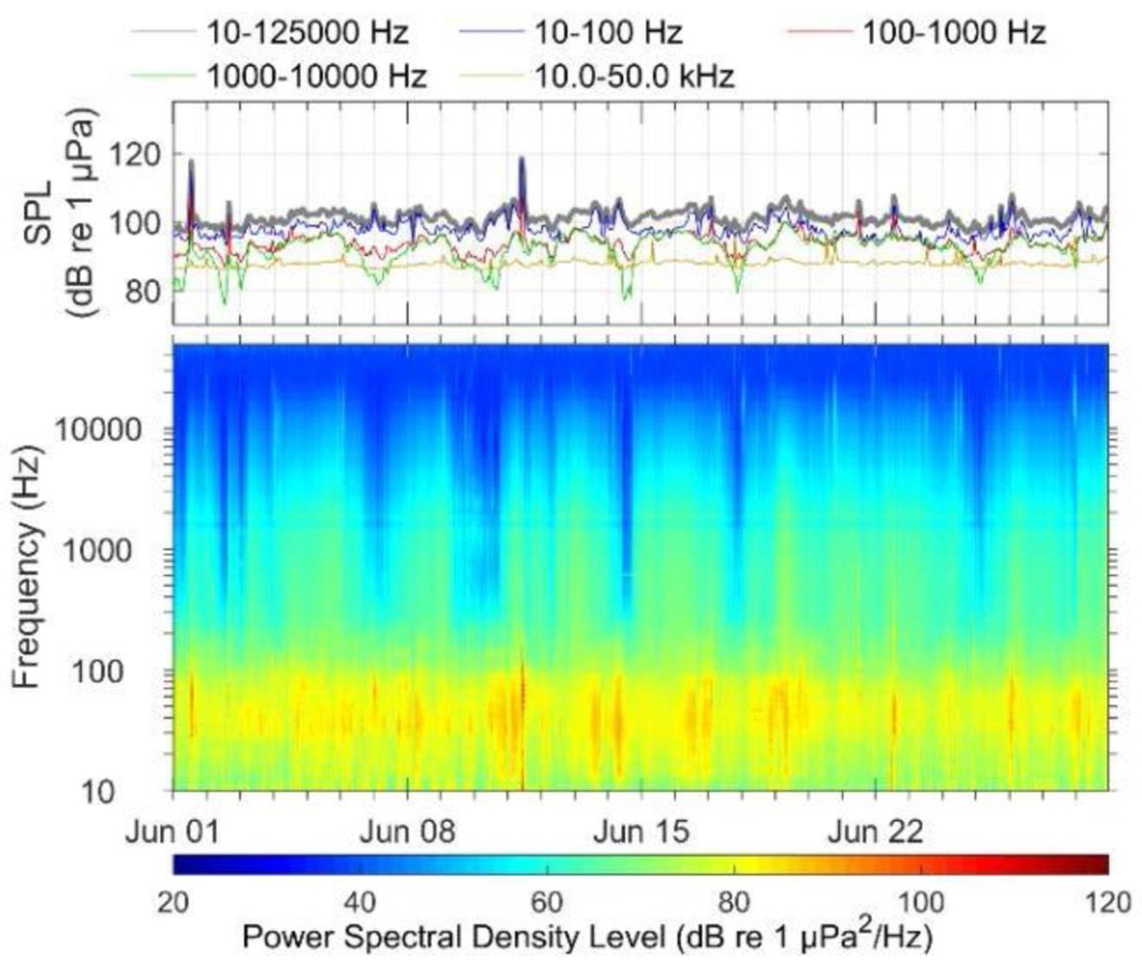
2.2. Acoustic Detections

2.2.1. Fin Whale Call Detections

Fin whale calls were identified using an automated detection algorithm and subsequently validated by experienced JASCO bio-acoustic experts. Cetacean tonal detectors were used to analyse moans and songs using predefined frequency bands for energy and contours. The spectrograms were analysed at 1 Hz resolution within a 0.2 s frame length and 0.05 s time step in a 5 s detection window with a detection threshold of 4. Fin whales were sorted from the data by recognizing call types between 17 and 40 Hz frequency range at 0.3–3 s duration and a bandwidth less than 6 including a minimum frequency of less than 17 Hz and sweep rate of −100 to 0 Hz/s. The maximum detection range for fin whale call detections was 200 km [26].
The automated detector performance and species occurrence were verified by JASCO bio-acoustic experts reviewing a selection of acoustic files visually and aurally. From each reviewed file, the presence or absence of identifiable moans of fin whales as well as shipping vessels was noted. The validation process was used to assess the performance of the automated detector to identify at least one moan in each file. Using the maximum likelihood estimator, the detection threshold (minimum number of automated detections in each file) was determined to optimise our results and maximise the F-score [31]:
F = ( 1 + β 2 )   P     R   ( β 2 ) P + R   ; P = T P T P + F P   ;   R = T P T P + F F
where the number of files with correctly detected calls (true positives; TP), incorrectly detected calls (false positive; FP), and missed calls (false negatives; FN) were used to compute the precision (P; proportion of correctly identified calls) and recall (the proportion of automatically detected calls) indices [26,31]. The significance of precision was emphasised over recall (β = 0.5) to increase the reliability of our results [26]. Therefore, the fin whale call presence/absence data used in this study represents the automated detections per acoustic file that equalled or exceeded the detection threshold as presence [31] and a failure to reach the threshold as absence [32].

2.2.2. Vessel Detections

In each minute of the data, dominant sound sources were classified as ‘ambient’ or ‘vessel’. Ambient sound levels were defined using one-minute average spectra of underwater sound data without anthropogenic detections for an hour on either side of the minute (using Hammond-windowed FFTs-120 times, 50% overlap window, and 1 Hz resolution). This led to more precise measurements from each source class for the daily sound exposure levels, cumulative distribution of sound pressure levels, and the exceedance spectra. Frequency bands of 10 Hz to 125 kHz, 10 to 100 Hz, 100 Hz to 1 kHz, 1 to 10 kHz, and 10 to 50 kHz were used to define the sound pressure level (SPL) of ambient noise over time. The one-minute sound exposure level (SEL) (linear sum of total received sound energy and detected shipping energy) values for shipping were multiplied by 60 s (duration) for linear one-minute squared SPL values. One-minute averaged broadband levels (dB re 1 μPa) were computed using one-minute averages of 1 Hz spectral density levels added over 1/3rd octave and decade bands [26].
The vessels in the region were detected in two steps. First, vessels were detected as tonals produced by the propulsion and other rotating systems (0.125 Hz resolution spectrogram window). Secondly, the root-mean-square (rms) of sound pressure levels (SPLs) evaluated for each minute in the 40–315 Hz frequency band (since mid- to large-sized vessels produce sounds in this range) were used as the received levels of shipping noise against the acoustic detections of fin whale calls as recommended by the MSFD (2008/56/EC) [2]. Vessel detections were confirmed if the SPL was 3 dB above the median but within 8 dB of the broadband SPL in the shipping band and at least 5 shipping tonals were present per minute (Figure 2) [26].

2.3. Environmental Data

To analyse habitat suitability, environmental data for the study site were downloaded from several online data archives. The mean values of sea surface salinity, sea bottom salinity, sea surface temperature, sea bottom temperature, mixed layer depth, and sea surface velocity for the duration of the study were accessed from the Marine Institute (Table 1). The European Union’s Copernicus Marine Environment Monitoring Service and NASA Ocean Colour Data provided information on sea surface height and chlorophyll-a concentration (as proxy for surface level phytoplankton biomass), respectively. Moderate Resolution Imaging Spectro-radiometer (MODIS) was used to generate data from the Aqua satellite. Temporal variables, such as the calendar month, day, hour, and partday (day-time (7 a.m.–7 p.m.)/night-time (7 p.m.–7 a.m.)), were also included in the habitat model.

2.4. Statistical Analysis

Using different exploratory graphs and analyses, normality, outliers, homogeneity, missing values, or collinearity between explanatory variables in the dataset were checked in R studio [33]. The dataset followed Bernoulli’s distribution (or binary distribution) as the independent response variable was the presence/absence data of fin whale call detections [34]. Presence-absence models were used as it has a higher explanatory and predictive power than presence-only models [35]. Generalized linear models (GLMs) in RStudio (RStudio Version 1.2.5042, Boston, MA, US) were used to account for the high zero inflation and binary nature of the data [36]. The logistic regression uses logit as the link function to determine the probability of the presence of fin whales in the region as shown below in Equation (1) [37]:
logit   p = log   o = log ( p / 1 p ) = β 0 + β 1   x 1 + β 2   x 2 + β 3   x 3 + β 4   x 4 + + β n x n  
Collinearity and correlations tests were used to remove variables with high collinearity using cor() and rcorr() from the “Hmisc” package. All the correlation coefficients were significant (p < 0.05) when tested with rcorr() function and the predictors with high correlation coefficients (>0.8) were dropped in this study (Figure 3).

2.5. Habitat Modelling

The model with significant variables (smallest p-value) was selected using forward selection, which tested each explanatory variable with the presence-absence data of fin whales to a null model. The final model with the lowest Akaike information criterion (AIC) was selected [24] and a chi-squared test was carried out to calibrate the significance of the variables in the final model. The variables ‘lat’, ‘lon’, ‘mld’, ‘sbs’, ‘sbt’, ‘sss’, ‘sst’, ‘ssxv’, and ‘ssyv’ (Table 1) were removed from the model after testing for its significance to avoid spatial correlation [38]. The final set of explanatory variables that contributed significantly towards the model were ‘rms’, ‘shptnl’, ‘month’, ‘day’, ‘hour’, ‘partday’, ‘ssh’, and ‘chlora’ (Table 1). An odds ratios table (97.5% CI) was generated to explain the effects of the per unit increase in the quantity of each variable on fin whale call detections as the coefficients from the summary() function only revealed if the detections were significantly different to the variables in the model.
The final habitat model with significant variables was validated with a repeated 10-fold (k-fold) cross-validation test to detect the prediction error rate [38]. The dataset was partitioned into 10 compartments and each time, a different compartment of data was trained using the model and the rest were tested for the effect to get a measure of accuracy and repeated 10 times [38]. Confusion matrices (confusionMatrix()) with a default probability threshold of 0.5 were used to tabulate the matrix with actual presence and absence data against predicted presence and absence data for the final model, predicting the probability of detection as absent below the threshold and the probability as present above it. Higher accuracy values (>0.5–1) imply the model fits the data better. False positives are when the model predicts the presence of a species when it was absent during observation (type I error) and true positives are when the model predicts the absence of a species when it was actually present during observation (type II error) [39]. The automated output from the R code for this data considered sensitivity (the ratio of correctly predicted presences by the total number of presences) value and specificity (ratio of correctly predicted absences to the total absences) value in an interchanged manner and hence were disregarded when evaluating the model [38,39]. Further, the model accuracy was estimated by calculating the area under the curve (AUC) value (ranges from 0–1, where a value > 0.5 implied higher accuracy) for a receiver operator curve (ROC) for the model [40]. The goodness of fit was calculated using McFadden’s pseudo r-squared where a value between 0.2 and 0.4 was considered extremely good [41]. Hypotheses tested in this study were that the temporal, environmental, and spatial variables have a significant effect on the presence of the fin whale species, thus testing if the habitat at the Irish shelf edge influences the presence of the fin whales and if shipping noise has an effect on the presence of the fin whale species.

3. Results

3.1. Detector Performance

The algorithm with the fixed validation effort was executed to automatically select around 1.6% of acoustic files, which was reviewed and manually validated by three experienced analysts. The automated detection results closely represent the acoustic occurrence of fin whales during periods of vocal activity with 81–100% correctly classified detections. The performance of the fin whale acoustic detectors was satisfactory with a 0.82 precision and 0.56 recall value with a classification threshold of 1 and an F-score threshold of 0.75 [26].

3.2. Observed Trends

Over the study period of 97 days, the average detection rate of fin whales was 46 detections per day and the detection positive minute (DPM) was 0.03194, i.e., the total number of minutes that detected fin whale calls in a day (Table 2). The highest percentage of fin whale call detections was observed during April (65.62%) and decreased from May (8.06%) through June (2.86%) (Table 3). On average, the number of shipping tonals was approximately 1365 per day and the shipping noise in the region during the study was 99.75 dB re 1 μPa/min (Table 3). Data indicates an increase in ambient noise between 99.75 dB (rms re 1 μPa/min) and 152.48 dB (rms re 1 μPa/min) due to high shipping activities in the offshore area and an increase in the number of fin whale call detections recorded from March to the end of April as well as an increase in shipping noise and a decrease in fin whale detections from May to July (Figure 4).

3.3. Habitat Modelling Results

The final habitat model had the lowest AIC compared to the other models and was considered a good fit for the data. All the variables included in this model, namely ‘rms’, ‘shptnl’, ‘day’, ‘hour’, ‘partdaynight’, ‘month’, ‘ssh’, and ‘chlora’ (Table 1), had a significant chi-squared (p ≤ 2.2 × 10⁻¹⁶), implying its importance in explaining the observed variability in fin whale call detections. Call detections varied significantly with temporal variables, such as months (p ≤ 2 × 10⁻¹⁶), days (p = 3.44 × 10⁻¹¹), hours (p = 5.59 × 10⁻⁸), and partday (p = 2.85 × 10⁻⁸), and the model showed that among all the temporal variables tested, the probability of detecting fin whale calls was higher during night-time (7 p.m.–7 a.m.) than day time (7 a.m.–7 p.m.) (partday (1.65)) (Table 4), indicating that fin whales were more acoustically active during the night.
Environmental variables, such as sea surface height (ssh) (p = 5.03 × 10⁻¹⁴) and chlorophyll-a concentration (chl-a) (p ≤ 2 × 10⁻¹⁶) (Table 4), had a significant effect on the fin whale calls. The call detections also significantly (p-value < 0.05) varied with the interaction of ssh and chl-a with the temporal variables (Table 4). The model predicted the probability of detecting fin whales was higher with every unit increase in ssh and chl-a in the region that depended on temporality. This means the probability of detecting whales was higher with increasing sea surface height, but an increase or decrease in detections was observed with varying sea surface height depending on temporality. Detections were predicted to decrease with sea surface height every night (0.33) but increase on an hourly basis (hour (0.92)) daily (day (0.94)) over the calendar months (month (0.75)) (Table 5). The results indicate a decrease in detections with a decrease in sea surface height every night but an increase in detection with an increase in sea surface height daily over the months. Similarly, the probability of detecting whales also increased with an increase in chlorophyll-a concentration on a daily temporal period (day (0.96)) but may decrease over the months (month (0.31)) (Table 5). This suggests the possibility of higher detections with an increase in chlorophyll-a concentration on a daily basis but decreases over the months.
Fin whale call detections significantly varied with shipping noise (rms dB re 1 μPa/min) (p ≤ 2 × 10⁻¹⁶) and the shipping tonals (p = 0.020) (Table 4). The odds ratios of these regressions (Table 4) suggested a strong decrease in the probability of detecting fin whales with every 1 dB re 1 μPa/min increase in noise levels (rms) (1.73) and with an increase in shipping tonal detections (0.95). The model predicted a gradual decrease in whale detections with increasing shipping noise over time, that is, the probability of detecting whales within increasing shipping noise during a day and over each week was higher (partday (1.06), hours (1.007), and days (0.99)) than the probability of detecting whales with increasing shipping noise over calendar months (months (0.88)) (Table 5). Overall, this indicated a possibility of lower fin whale call detections in the region with an increase in shipping noise over time.
Even though high model accuracy (0.95) was estimated using a repeated 10 stratified k-fold cross-validation method, a very high sensitivity (0.99), and a very low specificity (0.04) suggested the presence of a caveat in the model. The prediction worked better to accommodate absence of fin whale detections rather than presence, leading to a type II error [39]. Despite the type II error, the area under the curve (AUC) of the model was high (0.85) and significantly different from a random model (AUC = 0.5) under the receiver operator curve (ROC) (Figure 5), indicating high model accuracy. Further, McFadden’s pseudo-R squared of 0.25 also confirmed the model as an extremely well-fitting one. Hence, the habitat model was accepted to be a good fit, which indicated the acoustic presence of fin whales to be strongly influenced by shipping noise and primary productivity.

4. Discussion

This study provides insights into the acoustic presence of fin whales at Porcupine Ridge, keeping in mind that the spatial and temporal trends observed could be limited by the fact that the dataset only contributes information from the end of March 2016 to June 2016. Results of this study indicated the probability of higher acoustic activity of fin whales at night, potentially related to foraging. The call detections at Porcupine Ridge might be significantly influenced by specific environmental drivers like sea surface height and chlorophyll-a concentration. An important observation that addresses the hypothesis in this study is that the presence of shipping noise might have a significant impact on fin whale presence. However, the results must be interpreted cautiously as the final habitat model has a type II error, implying the model predicted the absence of species calls better than the presence. This could be rectified by increasing the effective sample size [42]. Possibly since presence/absence models do not take into account the migratory nature of long-ranging species like fin whales, it is difficult to state the presence of the species is limited to just one region [38].
Fin whales are known to occur year-round in the offshore Irish waters of the North Atlantic [43,44,45] and are sighted regularly, especially off the south coast along the Irish shelf edge according to study reports by the Irish Whale and Dolphin Group (2000–2009) [46]. A recent aerial study in 2018 reported overlap with prior evidence of interannual site fidelity through photo identification [47]. This is consistent with the fin whale occurrence on Porcupine Ridge. Usually, fin whale calls decrease from February to May through July as reported in previous literature [43,48]. Our study, however, revealed a trend of higher call detections in April decreasing from May to June. Some studies on baleen whales in the Azores showed similar peaks in April and speculated these regions may be ‘stop-over sites’ on the migratory route towards more productive northern regions during summer months [47,49]. Unfortunately, we do not have enough data or information to support this reasoning and would need interannual seasonal data to shed more light on this matter. The decreasing trend of fin whale call detections observed from May to June may be due to the auto detector having a lower detection success with song, resulting in a lower detection rate of calls [50]. Regular sightings of fin whales along the edges of the continental shelf during this period suggest the area might be an important foraging or migratory corridor [26,47], although long-term data with better habitat modelling techniques could be more revealing.
Fin whales have been observed to have a preference for shelf breaks, steep slopes, and ridges, most likely related to prey availability [51,52]. The steep elevated Porcupine Ridge marking a transition from a moderate depth (1000–2000 m) to deep waters (up to 4000m) along the southwestern Irish Atlantic Margin is part of the moderately productive Celtic-Biscay Shelf Large Marine Ecosystems (LME) influenced by the Shelf Slope Front (SSF) [53,54]. Topographical features like canyons and troughs along Porcupine Shelf causes instabilities in SSF [55], increasing the upwelling of nutrients influx from deep waters, and consequently, driving higher primary productivity coupled with higher prey availability in Porcupine Ridge, known to be preferred by baleen whales [56,57,58]. Baines et al. [12] confirmed that clusters of fin whales were sighted at Porcupine Seabight, presumably to exploit the seasonally abundant prey (northern krill).
Interestingly, our study revealed fin whales were more acoustically active during the night than the day due to prey availability, a common observation made in the Observe acoustic report [31] and other studies in the North Atlantic [59], Southern California Bight [60], and in the eastern North Pacific [13], associating higher fin whale calls during the night with foraging behaviour or social behaviour [50,61]. This higher acoustic activity of fin whales at night could be related to foraging dives due to the diurnal vertical migration (i.e., migration triggered by the change in light leading to the vertical movement of krill masses to the surface at night to feed and avoid predators) of their main prey, northern krill (Meganyctiphanes norvegica) [13,56,59,62]. Other baleen whales, such as the blue and sei whales, are also known to exhibit foraging dives at night [63,64,65]. An important note on this aspect is that since no data was collected on the northern krill in the region as a part of this study, we cannot pinpoint the biological link between higher vocal activities at night and foraging as it is beyond the scope of this study.
The findings of the present study demonstrated an increase in fin whale detections with increase in both sea surface height as well as chlorophyll-a concentration, which requires cautious interpretation as sea surface height and chlorophyll concentration are found to be inversely related, i.e., with increasing sea surface height, chlorophyll concentration decreased and vice versa [66]. Sea surface height might be an important factor in indicating the presence of fin whales as it is known to influence the oceanic fronts [57,58] like the SSF, which in turn promotes primary production and prey availability for fin whales to thrive in the region. Despite this, it is difficult to explain patterns of change observed in sea surface height with temporality and its link to call detections to any underlying biological significance with no comparable studies.
Chlorophyll-a concentration has been shown to be a good proxy to understand the prey availability [51,52,67] and hence could be considered as a strong predictor of fin whale presence [12,49]. As mentioned earlier, shelf breaks, such as the one at Porcupine Ridge with SSF, induce upwelling and downwelling of nutrients, boosting primary productivity due to the availability of chlorophyll-a in the water layers, leading to a higher abundance of northern krill as well as Clupea harengus (herring) and Sprattus sprattus (sprat) as alternate prey for fin whales present in the region [3,68]. Most likely, this could result in a spatial overlap between high densities of fishing vessels that target herring and sprat, and the baleen whales along the south and southwest coast of Ireland [3,45] that could lead to detrimental effects, such as higher noise in the region causing masking, entanglements, or bycatch of fin whales [8,69]. A catch in explaining the temporality observed in the results is the lag in the peaks of the chlorophyll-a concentration and zooplankton, which may take up to several weeks (up to 15) for fin whales to exploit as observed in previous literature [51,70]. Another possibility for the observed variation with temporality could be the fact that the SSF undergoes variation daily as well as seasonally, affecting the chlorophyll-a concentration [26,54]. Regardless, this study did not collect real-time data on prey species during the survey to provide conclusions on the complex predator–prey relationship in fin whales in the presence of chlorophyll concentration. We, therefore, recommend that to provide a better analysis, long-term data should be collected on the environmental drivers and prey species for fin whales [51].
Notable increases in ambient noise levels were seen as a result of shipping activities and exposures to sound pressure levels higher than 120 dB (rms re 1 μPa/min) may cause significant disturbance to cetaceans along the Irish shelf edge [71]. Our study suggests a decline in fin whale call detection rates with an increase in shipping noise over time, which has also been noted in previous studies [72]. Studies in the Azores highlight the possibility of an increase in masking of fin whale calls with higher vessel noise in the region [73,74]. Thus, indicating fin whales to be sensitive to changes in ambient noise. However, it cannot be concluded that the fin whale call detections were indeed very low only due to the presence of vessel noise as there might be several underlying factors. The exact direction and position of the whales and shipping vessels were unknown and the presence of variations due to natural sounds and sound propagation in water were unaccounted for in this study, which could have induced any observed variability of detections. The low detection of fin whale calls could be as a result of masking or voluntary cessation of vocalisations (triggering false absence, i.e., non-detection of species when they are actually present) by whales. Alternatively, it is likely that the whales temporarily abandoned the region to avoid vessels (true absence, i.e., non-detection of species as the whales are actually not present in the region). Future studies can also investigate the shadow effect of the continental slope on the shelf near the bottom where the AMAR was deployed as this was not accounted for in this study but could affect the detection ranges of fin whales.
Several studies in baleen whales, such as the fin, blue (Balaenoptera musculus), right (Eubalaena), Bryde’s (Balaenoptera brydei), and minke (Balaenoptera acutorostrata) whales, have shown a reduction and fragmentation in communication space as a consequence of masking potentially incurring detrimental impacts on communication and breeding activities [1,4,23,75,76]. Another impact is the abandonment of a preferred or critical habitat, such as the breeding ground as observed in gray whales (Eschrichtius robustus), to evade the high shipping and dredging activities [77] and returning only years after the industry closed [78,79]. Such compensations come with high energy costs, compromising the foraging and reproductive success, thus jeopardising the survival of the population [4,21,80]. Nonetheless, a study by Croll et al. [8] found that even with received levels of around 140 dB re 1 μPa, the presence of fin whales may not be affected but could strongly be driven by prey availability in the region. Therefore, it is essential to explore the importance of Porcupine Ridge as a suitable habitat for fin whales to set up noise monitoring and impact management in Irish waters.
Habitat modelling in a regional scope to predict accurate space use is strongly influenced by the availability of cetacean data making it challenging to conclude the complex interconnections between the physical, temporal, spatial, and biological distributions from the environmental data [81]. The modelling approach in this study may have missed a few unknown predictors and might have simplified the intricate relationship between cetaceans and their environment. To increase the statistical robustness, other approaches, such as GAMMs, can be used with long-term data to understand the extent of habitat use, and GEEs to correct for temporal autocorrelation in the data instead of just using k-fold partitioning to assess the accuracy of the model [32]. With the known occurrence of fin whales in the region from this and previous studies and the presence of high commercial interests, it is safe to suggest further monitoring of fin whales and vessels over time to understand the biological importance of Porcupine Ridge as a habitat. Consequently, understanding the habitat preferences over temporal and spatial scales is crucial in recognizing ‘critical habitats’ for these vulnerable species that migrate long distances to forage and breed [82]. Future research aimed at exploring this connectivity between complex anthropogenic and ecological interactions should include visual monitoring, shipping and fishing vessel data (AIS), as well as all the environmental with spatio-temporal predictors to establish an ecosystem-based management plan [83,84,85]. Information from this study can be used as a baseline to gather appropriate data required to inform the impacts of increasing underwater noise monitored under the MSFD guidelines and to identify critical habitats to help in the management and conservation of fin whale species under the EU Habitat Directive.

Author Contributions

Conceptualization, S.B., R.M. and J.O.; methodology, S.B., R.M. and J.O.; software, J.O.; validation, J.O.; formal analysis, K.R.; investigation, K.R.; resources, K.R.; data curation, S.B., R.M., J.O. and K.R.; writing—original draft preparation, K.R. and J.O.; writing—review and editing, K.R., S.B., R.M. and J.O.; visualization, K.R.; supervision, J.O.; project administration, S.B., R.M. and J.O.; funding acquisition, S.B. and J.O. All authors have read and agreed to the published version of the manuscript.

Funding

This research was funded by the Department of Communications, Climate Action and Environment in partnership with the Department of Culture, Heritage, and the Gaeltacht under Ireland’s ObSERVE Programme.

Institutional Review Board Statement

Not applicable.

Informed Consent Statement

Not applicable.

Data Availability Statement

Restrictions apply to the availability of these data. Data is owned by the Irish Department of Communications, Climate Action and Environment and requests for access to the raw acoustic data can be submitted to [email protected].

Acknowledgments

We would like to thank the captains and crews of RV Celtic Voyager and RV Celtic Explorer for providing support to deploy and retrieve the AMARs. Many thanks to John Barry, Jessica Ridge and Anthony English of P&O Maritime Ireland and Michael Marrinan for providing support during the Static Acoustic Monitoring deployments and recoveries. Many thanks to the team from JASCO for the initial analysis of the AMAR data. We would like to thank Sharon Creaton, Aoife Tuohy, Deirdre Duffy-Carthy, Noreen Kelly, Fionnuala Kelly and Maura Gilligan of the Galway-Mayo Institute of Technology for their administrative support throughout the project. Oceanographic data was provided by the Marine Institute, Copernicus and the Ocean Biology Processing Group at NASA.

Conflicts of Interest

The authors declare no conflict of interest.

References

  1. Hatch, L.T.; Clark, C.W.; Van Parijs, S.M.; Frankel, A.S.; Ponirakis, D.W. Quantifying Loss of Acoustic Communication Space for Right Whales in and around a U.S. National Marine Sanctuary. Conserv. Biol. 2012, 26, 983–994. [Google Scholar] [CrossRef]
  2. André, M.; Van der Schaar, M.; Zaugg, S.; Houégnigan, L.; Sánchez, A.M.; Castell, J.V. Listening to the Deep: Live monitoring of ocean noise and cetacean acoustic signals. Mar. Pollut. Bull. 2011, 63, 18–26. [Google Scholar] [CrossRef] [PubMed] [Green Version]
  3. Beck, S.; O’Brien, J.; Berrow, S.; O’Connor, I.; Wall, D. Assessment of Impulsive and Continuous Low-Frequency Noise in Irish Waters. In The Effects of Noise on Aquatic Life II; Popper, A.N., Hawkins, A., Eds.; Springer: New York, NY, USA, 2016; pp. 73–81. Available online: http://link.springer.com/10.1007/978-1-4939-2981-8_9 (accessed on 24 May 2020).
  4. Clark, C.W.; Ellison, W.T.; Southall, B.L.; Hatch, L.; Van Parijs, S.M.; Frankel, A.; Ponirakis, D. Acoustic masking in marine ecosystems: Intuitions, analysis, and implication. Mar. Ecol. Progress Ser. 2009, 395, 201–222. [Google Scholar] [CrossRef]
  5. Southall, B.; Bowles, A.; Ellison, W.; Finneran, J.; Gentry, R.; Greene, C., Jr.; Kastak, D.; Ketten, D.; Miller, J.; Nachtigall, P.; et al. Marine Mammal Noise Exposure Criteria: Initial Scientific Recommendations. Bioacoustics 2008, 17, 273–275. [Google Scholar] [CrossRef]
  6. Studds, G.E.; Wright, A.J. A Brief Review of Anthropogenic Sound in the Oceans. Int. J. Comp. Psychol. 2007, 20, 14. [Google Scholar]
  7. Wright, A.J.; Deak, T.; Parsons, E.C.M. Concerns related to chronic stress in marine mammals. Int. Whal. Comm. 2009, 2, 1–7. [Google Scholar]
  8. Croll, D.A.; Clark, C.W.; Calambokidis, J.; Ellison, W.T.; Tershy, B.R. Effect of anthropogenic low-frequency noise on the foraging ecology of Balaenoptera whales. Anim. Conserv. 2001, 4, 13–27. [Google Scholar] [CrossRef] [Green Version]
  9. Tennessen, J.; Parks, S. Acoustic propagation modeling indicates vocal compensation in noise improves communication range for North Atlantic right whales. Endang. Species Res. 2016, 30, 225–237. [Google Scholar] [CrossRef] [Green Version]
  10. Nowacek, D.P.; Thorne, L.H.; Johnston, D.W.; Tyack, P.L. Responses of cetaceans to anthropogenic noise. Mammal Rev. 2007, 37, 81–115. [Google Scholar] [CrossRef]
  11. Tyack, P.L. Implications for marine mammals of large-scale changes in the marine acoustic environment. J. Mammal. 2008, 89, 549–558. [Google Scholar] [CrossRef] [Green Version]
  12. Baines, M.; Reichelt, M.; Griffin, D. An autumn aggregation of fin (Balaenoptera physalus) and blue whales (B. musculus) in the Porcupine Seabight, southwest of Ireland. Deep Sea Res. Part II Top. Stud. Oceanogr. 2017, 141, 168–177. [Google Scholar] [CrossRef]
  13. Širović, A.; Williams, L.N.; Kerosky, S.M.; Wiggins, S.M.; Hildebrand, J.A. Temporal separation of two fin whale call types across the eastern North Pacific. Mar. Biol. 2013, 160, 47–57. [Google Scholar] [CrossRef] [Green Version]
  14. Víkingsson, G.A.; Pike, D.G.; Desportes, G.; Øien, N.; Gunnlaugsson, T.; Bloch, D. Distribution and abundance of fin whales (Balaenoptera physalus) in the Northeast and Central Atlantic as inferred from the North Atlantic Sightings Surveys 1987–2001. NAMMCO Sci. Publ. 2009, 7, 49–72. [Google Scholar] [CrossRef] [Green Version]
  15. Hammond, P.S.; Macleod, K.; Berggren, P.; Borchers, D.L.; Burt, L.; Cañadas, A.; Desportes, G.; Donovan, G.P.; Gilles, A.; Gillespie, D.; et al. Cetacean abundance and distribution in European Atlantic shelf waters to inform conservation and management. Biol. Conserv. 2013, 164, 107–122. [Google Scholar] [CrossRef] [Green Version]
  16. McCauley, R.D. Offshore Irish Noise Logger Program (March to September 2014): Analysis of Cetacean Presence, and Ambient and Anthropogenic Noise Sources. Centre for Marine Science and Technology (CMST), Curtin University For RPS MetOcean/Woodside Energy (Ireland) Pty Ltd. 2015. Available online: https://cmst.curtin.edu.au/wp-content/uploads/sites/4/2015/06/CMST-2015-01-1296-Ireland-DRIMS_10574111.pdf (accessed on 14 August 2020).
  17. O’Brien, J.; Berrow, S.; McGrath, D.; Evans, P. Cetaceans In Irish Waters: A Review of Recent Research. Biol. Environ. Proc. R. Ir. Acad. 2009, 109B, 63–88. [Google Scholar] [CrossRef] [Green Version]
  18. Wall, D.; O’Brien, J.; Meade, J.; Allen, B.M. Summer Distribution and Relative Abundance of Cetaceans off the West Coast of Ireland. Biol. Environ. Proc. R. Ir. Acad. 2006, 106, 135–142. [Google Scholar] [CrossRef] [Green Version]
  19. Clapham, P.J.; Young, S.B.; Brownell, R.L. Baleen whales: Conservation issues and the status of the most endangered populations. Mammal Rev. 1999, 29, 37–62. [Google Scholar] [CrossRef] [Green Version]
  20. Payne, R.; Webb, D. Orientation by means of long range acoustic signalling in baleen whales. Ann. N. Y. Acad. Sci. 1971, 188, 110–141. [Google Scholar] [CrossRef]
  21. Castellote, M.; Clark, C.W.; Lammers, M.O. Acoustic and behavioural changes by fin whales (Balaenoptera physalus) in response to shipping and airgun noise. Biol. Conserv. 2012, 147, 115–122. [Google Scholar] [CrossRef]
  22. Romagosa, M.; Pérez-Jorge, S.; Cascão, I.; Mouriño, H.; Lehodey, P.; Pereira, A.; Marques, T.A.; Matias, L.; Silva, M.A. Food talk: 40-Hz fin whale calls are associated with prey biomass. Proc. R. Soc. B 2021, 288, 20211156. [Google Scholar] [CrossRef]
  23. Cholewiak, D.; Clark, C.W.; Ponirakis, D.; Frankel, A.; Hatch, L.T.; Risch, D.; Stanistreet, J.E.; Thompson, M.; Vu, E.; Van Parijs, S.M. Communicating amidst the noise: Modeling the aggregate influence of ambient and vessel noise on baleen whale communication space in a national marine sanctuary. Endang. Species Res. 2018, 36, 59–75. [Google Scholar] [CrossRef] [Green Version]
  24. Praca, E.; Gannier, A.; Das, K.; Laran, S. Modelling the habitat suitability of cetaceans: Example of the sperm whale in the northwestern Mediterranean Sea. Deep Sea Res. Part I Oceanogr. Res. Pap. 2009, 56, 648–657. [Google Scholar] [CrossRef]
  25. Redfern, J.V.; Ferguson, M.C.; Becker, E.A.; Hyrenbach, K.D.; Good, C.; Barlow, J.; Kaschner, K.; Baumgartner, M.F.; Forney, K.A.; Ballance, L.T.; et al. Techniques for cetacean–habitat modeling. Mar. Ecol. Progress Ser. 2006, 310, 271–295. [Google Scholar] [CrossRef]
  26. Berrow, S.; O’Brien, J.; Meade, R.; Delarue, J.; Kowarski, K.; Martin, B.; Moloney, J.; Wall, D.; Gillespie, D.; Leaper, R.; et al. Acoustic Surveys of Cetaceans in the Irish Atlantic Margin in 2015–2016: Occurrence, Distribution and Abundance; Department of Communication, Climate Action and Environment: Dublin, Ireland, 2018; 354p. [Google Scholar]
  27. Mellinger, D.; Barlow, J. Future Directions for Acoustic Marine Mammal Surveys: Stock Assessment and Habitat Use: Report of a workshop Held in La Jolla, California, 20-22 November 2002; NOAA Pacific Marine Environmental Laboratory: Seattle, WA, USA, 2003; p. 45, Report No.: Technical contribution No. 2557. [Google Scholar]
  28. O’Brien, J.; Beck, S.; Wall, D.; Pierini, A. Marine Mammals and Megafauna in Irish Waters—Behaviour, Distribution and Habitat Use-WP 2: Developing Acoustic Monitoring Techniques; Marine Institute: Galway, Ireland, 2013. [Google Scholar]
  29. Van der Graaf, A.; Ainslie, M.; André, M.; Brensing, K.; Dalen, J.; Dekeling, R.P.; Robinson, S.; Tasker, M.L.; Thomsen, F.; Werner, S. 2012, p. 27. Available online: https://ec.europa.eu/environment/marine/pdf/MSFD_reportTSG_Noise.pdf (accessed on 15 July 2021).
  30. Moloney, J.; Hillis, C.; Mouy, X.; Urazghildiiev, I.; Dakin, T. Autonomous Multichannel Acoustic Recorders on the VENUS Ocean Observatory. In 2014 Oceans—St John’s; IEEE: St. John’s, NL, Canada, 2014; pp. 1–6. Available online: http://ieeexplore.ieee.org/document/7003201/ (accessed on 30 October 2019).
  31. Kowarski, K.; Delarue, J.; Martin, B.; O’Brien, J.; Meade, R.; Ó Cadhla, O.; Berrow, S. Signals from the deep: Spatial and temporal acoustic occurrence of beaked whales off western Ireland. PLoS ONE 2018, 13, e0199431. [Google Scholar] [CrossRef] [PubMed]
  32. Barile, C.; Berrow, S.; O’Brien, J. Oceanographic Drivers of Cuvier’s (Ziphius cavirostris) and Sowerby’s (Mesoplodon bidens) Beaked Whales Acoustic Occurrence along the Irish Shelf Edge. J. Mar. Sci. Eng. 2021, 9, 1081. [Google Scholar] [CrossRef]
  33. R Core Team. R: A Language and Environment for Statistical Computing (Computer Software). Vienna, Austria. 2020. Available online: https://www.R-project.org (accessed on 15 July 2021).
  34. James, G.; Witten, D.; Hastie, T.; Tibshirani, R. An Introduction to Statistical Learning; Springer: New York, NY, USA, 2013; Springer Texts in Statistics; Volume 103, Available online: http://link.springer.com/10.1007/978-1-4614-7138-7 (accessed on 12 May 2020).
  35. Brotons, L.; Thuiller, W.; Araújo, M.B.; Hirzel, A.H. Presence-absence versus presence-only modelling methods for predicting bird habitat suitability. Ecography 2004, 27, 437–448. [Google Scholar] [CrossRef] [Green Version]
  36. Zuur, A.F.; Ieno, E.N.; Smith, G.M. Analysing Ecological Data; Statistics for Biology and Health; Springer: New York, NY, USA; London, UK, 2007; 672p. [Google Scholar]
  37. Manning, C. Logistic regression (with R). Changes 2007, 4, 1–15. [Google Scholar]
  38. Fielding, A.H.; Bell, J.F. A review of methods for the assessment of prediction errors in conservation presence/absence models. Environ. Conserv. 1997, 24, 38–49. [Google Scholar] [CrossRef]
  39. Jiménez-Valverde, A.; Lobo, J.M. Threshold criteria for conversion of probability of species presence to either–or presence–absence. Acta Oecol. 2007, 31, 361–369. [Google Scholar] [CrossRef]
  40. Hjort, J.; Luoto, M. Can abundance of geomorphological features be predicted using presence–absence data? Earth Surf. Process. Landforms 2008, 33, 741–750. [Google Scholar] [CrossRef]
  41. Louviere, J.J.; Hensher, D.A.; Swait, J.D.; Adamowicz, W. Stated Choice Methods: Analysis and Applications, 1st ed.; Cambridge University Press: Cambridge, UK, 2000; Available online: https://www.cambridge.org/core/product/identifier/9780511753831/type/book (accessed on 18 May 2020).
  42. Prajapati, B.; Dunne, M.; Armstrong, R. Sample size estimation and statistical power analyses. Optom. Today 2010, 16, 10–18. [Google Scholar]
  43. Delarue, J.; Todd, S.K.; Van Parijs, S.M.; Di Iorio, L. Geographic variation in Northwest Atlantic fin whale (Balaenoptera physalus) song: Implications for stock structure assessment. J. Acoust. Soc. Am. 2009, 125, 1774–1782. [Google Scholar] [CrossRef] [PubMed]
  44. Morano, J.L.; Salisbury, D.P.; Rice, A.N.; Conklin, K.L.; Falk, K.L.; Clark, C.W. Seasonal and geographical patterns of fin whale song in the western North Atlantic Ocean. J. Acoust. Soc. Am. 2012, 132, 1207–1212. [Google Scholar] [CrossRef] [PubMed]
  45. Whooley, P.; Berrow, S.; Barnes, C. Photo-identification of fin whales (Balaenoptera physalus L.) off the south coast of Ireland. Mar. Biodivers. Rec. 2011, 4, e8. [Google Scholar] [CrossRef]
  46. Berrow, S.; Whooley, P.; Irish Whale and Dolphin Group, Irish Scheme for Cetacean Observation and Public Education. Irish Cetacean Review (2000–2009): A Review of All Cetacean Sighting and Stranding Records Made during the Period 2000–2009 by the IWDG through ISCOPE, the Irish Scheme for Cetacean Observation and Public Education; IWDG: Kilrush, Ireland, 2010. [Google Scholar]
  47. Rogan, E.; Breen, P.; Mackey, M.; Cañadas, A.; Scheidat, M.; Geelhoed, S.C.V.; Jessopp, M. Aerial Surveys of Cetaceans and Seabirds in Irish waters: Occurrence, distribution and abundance in 2015–2017; Department of Communications, Climate Action & Environment: Dublin, Ireland, 2018. [Google Scholar]
  48. Chariff, R.A.; Clark, C.W. Acoustic Monitoring of Large Whales in Deep Waters North and West of the British Isles: 1996–2005. Cornell Laboratory of Ornithology. 2009; p. 40. Available online: https://assets.publishing.service.gov.uk/government/uploads/system/uploads/attachment_data/file/196484/OES_UK_SOSUS_10year_report.pdf (accessed on 4 August 2020).
  49. Prieto, R.; Tobeña, M.; Silva, M.A. Habitat preferences of baleen whales in a mid-latitude habitat. Deep Sea Res. Part II Top. Stud. Oceanogr. 2017, 141, 155–167. [Google Scholar] [CrossRef]
  50. Watkins, W.A.; Tyack, P.; Moore, K.E.; Bird, J.E. The 20-Hz signals of finback whales (Balaenoptera physalus). J. Acoust. Soc. Am. 1987, 82, 1901–1912. [Google Scholar] [CrossRef]
  51. Panigada, S.; Zanardelli, M.; MacKenzie, M.; Donovan, C.; Mélin, F.; Hammond, P.S. Modelling habitat preferences for fin whales and striped dolphins in the Pelagos Sanctuary (Western Mediterranean Sea) with physiographic and remote sensing variables. Remote. Sens. Environ. 2008, 112, 3400–3412. [Google Scholar] [CrossRef]
  52. Scales, K.L.; Schorr, G.S.; Hazen, E.L.; Bograd, S.J.; Miller, P.I.; Andrews, R.D.; Zerbini, A.N.; Falcone, E.A. Should I stay or should I go? Modelling year-round habitat suitability and drivers of residency for fin whales in the California Current. Divers. Distrib. 2017, 23, 1204–1215. [Google Scholar] [CrossRef] [Green Version]
  53. Dransfeld, L.; Maxwell, H.W.; Moriarty, M.; Nolan, C.; Kelly, E.; Pedreschi, D.; Slattery, N.; Connolly, P. North Western Waters Atlas, 3rd ed.; Marine Institute: Galway, Ireland, 2015; Available online: https://oar.marine.ie/handle/10793/1075 (accessed on 4 June 2020).
  54. White, M.; Bowyer, P. The Shelf-Edge Current North-West of Ireland. In Annales Geophysicae; Springer: Berlin/Heidelberg, Germany, 1997; Volume 15, pp. 1076–1083. [Google Scholar]
  55. Belkin, I.M.; Cornillon, P.C. Fronts in the World Ocean’s Large Marine Ecosystems. ICES CM 2007, 500, 21–33. [Google Scholar]
  56. Baines, M.E.; Reichelt, M. Upwellings, canyons and whales: An important winter habitat for balaenopterid whales off Mauritania, northwest Africa. J. Cetacean Res. Manag. 2014, 14, 57–67. [Google Scholar]
  57. Shabangu, F.W.; Findlay, K.P.; Yemane, D.; Stafford, K.M.; Van den Berg, M.; Blows, B.; Andrew, R.K. Seasonal occurrence and diel calling behaviour of Antarctic blue whales and fin whales in relation to environmental conditions off the west coast of South Africa. J. Mar. Syst. 2019, 190, 25–39. [Google Scholar] [CrossRef]
  58. Shabangu, F.W.; Yemane, D.; Stafford, K.M.; Ensor, P.; Findlay, K.P. Modelling the effects of environmental conditions on the acoustic occurrence and behaviour of Antarctic blue whales. PLoS ONE 2017, 12, e0172705. [Google Scholar] [CrossRef] [PubMed]
  59. Víkingsson, G.A. Feeding of fin whales (Balaenoptera physalus) off Iceland—Diurnal and seasonal variation and possible rates. J. Northwest Atl. Fish. Sci. 1997, 77–89. [Google Scholar] [CrossRef]
  60. Keen, E.M.; Falcone, E.A.; Andrews, R.D.; Schorr, G.S. Diel Dive Behavior of Fin Whales (Balaenoptera physalus) in the Southern California Bight. Aquat. Mamm. 2019, 45, 233–243. [Google Scholar] [CrossRef]
  61. Simon, M.; Stafford, K.M.; Beedholm, K.; Lee, C.M.; Madsen, P.T. Singing behavior of fin whales in the Davis Strait with implications for mating, migration and foraging. J. Acoust. Soc. Am. 2010, 128, 3200–3210. [Google Scholar] [CrossRef] [Green Version]
  62. Christie, A.E.; Yu, A.; Pascual, M.G. Circadian signaling in the Northern krill Meganyctiphanes norvegica: In silico prediction of the protein components of a putative clock system using a publicly accessible transcriptome. Mar. Genomics 2018, 37, 97–113. [Google Scholar] [CrossRef]
  63. Baumgartner, M.F.; Fratantoni, D.M. Diel periodicity in both sei whale vocalization rates and the vertical migration of their copepod prey observed from ocean gliders. Limnol. Oceanogr. 2008, 53, 2197–2209. [Google Scholar] [CrossRef] [Green Version]
  64. Stafford, K.M.; Moore, S.E.; Fox, C.G. Diel variation in blue whale calls recorded in the eastern tropical Pacific. Anim. Behav. 2005, 69, 951–958. [Google Scholar] [CrossRef]
  65. Wiggins, S.; Oleson, E.; Mcdonald, M.; Hildebrand, J. Blue Whale (Balaenoptera musculus) Diel Call Patterns Offshore of Southern California. Aquat. Mamm. 2005, 31, 161–168. [Google Scholar] [CrossRef]
  66. Pastor, M.V.; Palter, J.B.; Pelegrí, J.L.; Dunne, J.P. Physical drivers of interannual chlorophyll variability in the eastern subtropical North Atlantic: Interannual Chlorophyll Variability. J. Geophys. Res. Oceans 2013, 118, 3871–3886. [Google Scholar] [CrossRef] [Green Version]
  67. Druon, J.N.; Panigada, S.; David, L.; Gannier, A.; Mayol, P.; Arcangeli, A.; Cañadas, A.; Laran, S.; Di Méglio, N.; Gauffier, P. Potential feeding habitat of fin whales in the western Mediterranean Sea: An environmental niche model. Mar. Ecol. Progress Ser. 2012, 464, 289–306. [Google Scholar] [CrossRef] [Green Version]
  68. Ryan, C.; Berrow, S.D.; McHugh, B.; O’Donnell, C.; Trueman, C.N.; O’Connor, I. Prey preferences of sympatric fin (Balaenoptera physalus) and humpback (Megaptera novaeangliae) whales revealed by stable isotope mixing models. Mar. Mamm. Sci. 2014, 30, 242–258. [Google Scholar] [CrossRef]
  69. Thomas, P.O.; Reeves, R.R.; Brownell, R.L. Status of the world’s baleen whales. Mar. Mamm. Sci. 2016, 32, 682–734. [Google Scholar] [CrossRef] [Green Version]
  70. Visser, F.; Hartman, K.; Pierce, G.; Valavanis, V.; Huisman, J. Timing of migratory baleen whales at the Azores in relation to the North Atlantic spring bloom. Mar. Ecol. Progress Ser. 2011, 440, 267–279. [Google Scholar] [CrossRef] [Green Version]
  71. NRC (Ed.) Marine Mammal Populations and Ocean Noise: Determining when Noise Causes Biologically Significant Effects; National Academies Press: Washington, DC, USA, 2005; 126p. [Google Scholar]
  72. Sciacca, V.; Caruso, F.; Beranzoli, L.; Chierici, F.; De Domenico, E.; Embriaco, D.; Favali, P.; Giovanetti, G.; Larosa, G.; Marinaro, G. Annual Acoustic Presence of Fin Whale (Balaenoptera physalus) Offshore Eastern Sicily, Central Mediterranean Sea. PLoS ONE 2015, 10, e0141838. [Google Scholar] [CrossRef] [PubMed] [Green Version]
  73. Romagosa, M.; Cascão, I.; Silva, M.A. Underwater noise levles and shipping off the Faial–Pico Channel, Azores, in relation to the acoustic presence of baleen whales. Acústica 2020, 23, 1–9. [Google Scholar]
  74. Romagosa, M.; Cascão, I.; Merchant, N.D.; Lammers, M.O.; Giacomello, E.; Marques, T.A.; Silva, M.A. Underwater Ambient Noise in a Baleen Whale Migratory Habitat Off the Azores. Front. Mar. Sci. 2017, 4, 109. [Google Scholar] [CrossRef] [Green Version]
  75. Aulanier, F.; Simard, Y.; Roy, N.; Bandet, M.; Gervaise, C. Groundtruthed probabilistic shipping noise modeling and mapping: Application to blue whale habitat in the Gulf of St. Lawrence. Proc. Mtgs. Acoust. 2016, 070006. Available online: http://asa.scitation.org/doi/abs/10.1121/2.0000258 (accessed on 28 May 2020).
  76. Gabriele, C.M.; Ponirakis, D.W.; Clark, C.W.; Womble, J.N.; Vanselow, P.B.S. Underwater Acoustic Ecology Metrics in an Alaska Marine Protected Area Reveal Marine Mammal Communication Masking and Management Alternatives. Front. Mar. Sci. 2018, 5, 270. [Google Scholar] [CrossRef]
  77. Dahlheim Marilyn, E.; Dean Fisher, H.; Schempp, J.D. The Gray Whale: Eschrichtius Robustus, 1st ed.; Academic Press: Cambridge, MA, USA, 1984; pp. 511–541. Available online: https://www.elsevier.com/books/the-gray-whale-eschrichtius-robustus/jones/978-0-08-092372-7 (accessed on 17 August 2020).
  78. Bryant, P.J.; Lafferty, C.M.; Lafferty, S.K. Reoccupation of Laguna Guerrero Negro, Baja California, Mexico, by Gray Whales. In The Gray Whale: Eschrichtius Robustus; Elsevier: Amsterdam, The Netherlands, 1984; pp. 375–387. Available online: https://linkinghub.elsevier.com/retrieve/pii/B9780080923727500212 (accessed on 17 August 2020).
  79. Jones, M.L.; Swartz, S.L.; Leatherwood, S. The Gray Whale: Eschrichtius Robustus; Academic Press: Cambridge, MA, USA, 2012; 625p. [Google Scholar]
  80. Beale, C.M. The Behavioral Ecology of Disturbance Responses. Int. J. Comp. Psychol. 2007, 20, 11. [Google Scholar]
  81. Scales, K.L.; Hazen, E.L.; Jacox, M.G.; Edwards, C.A.; Boustany, A.M.; Oliver, M.J.; Bograd, S.J. Scale of inference: On the sensitivity of habitat models for wide-ranging marine predators to the resolution of environmental data. Ecography 2017, 40, 210–220. [Google Scholar] [CrossRef]
  82. Pirotta, E.; Matthiopoulos, J.; MacKenzie, M.; Scott-Hayward, L.; Rendell, L. Modelling sperm whale habitat preference: A novel approach combining transect and follow data. Mar. Ecol. Progress Ser. 2011, 436, 257–272. [Google Scholar] [CrossRef] [Green Version]
  83. Daly, E.; White, M. Bottom trawling noise: Are fishing vessels polluting to deeper acoustic habitats? Mar. Pollut. Bull. 2021, 162, 111877. [Google Scholar] [CrossRef] [PubMed]
  84. Katsanevakis, S.; Stelzenmüller, V.; South, A.; Sørensen, T.K.; Jones, P.J.; Kerr, S.; Badalamenti, F.; Anagnostou, C.; Breen, P.; Chust, G.; et al. Ecosystem-based marine spatial management: Review of concepts, policies, tools, and critical issues. Ocean Coast. Manag. 2011, 54, 807–820. [Google Scholar] [CrossRef] [Green Version]
  85. Merchant, N.D.; Pirotta, E.; Barton, T.R.; Thompson, P.M. Monitoring ship noise to assess the impact of coastal developments on marine mammals. Mar. Pollut. Bull. 2014, 78, 85–95. [Google Scholar] [CrossRef] [PubMed] [Green Version]
Figure 1. Map showing the position of mooring 6 (latitude 51.72257 and longitude −15.20771) at Porcupine Ridge along the Irish Shelf Edge off western Ireland of the study site.
Jmse 09 01207 g001
Figure 2. In-band SPL (top) and spectrogram (bottom) of underwater sound in June 2016 at Mooring 6 (reproduced from ObSERVE Programme Report [26], with permission from Department of Communication, Climate Action and Environment, 2018).
Jmse 09 01207 g002
Figure 3. This correlogram was plotted using the corrplot() function (“corrplot” package). The size of the circle is directly proportional to the correlation coefficients while blue represents the positive correlations and red the negative. This figure indicates the measure of collinearity between the different variables used in the modelling.
Jmse 09 01207 g003
Figure 4. Time series graph showing variation of fin whale detections (FW) and shipping detections (shptnl) recorded over the period of study.
Jmse 09 01207 g004
Figure 5. The graph depicts the ROC curve for the final fin whale model. The blue-coloured line depicts a better fit with an AUC = 0.85 than the red line, which represents the model with only shipping noise as an explanatory variable with a much lower AUC = 0.68. The diagonal black line indicates the chance model shows no discrimination with AUC = 0.5.
Jmse 09 01207 g005
Table 1. Description of variables used in the analysis along with its sources where applicable.
VariableDescriptionUnitSourcesVariable Type
FWbiFin whale detection presence/absencepresence/absence per minRecorded from AMARIndependent
shptnlNumber of shipping tonal detectionsDetections/minRecorded from AMARDependent
rmsRoot mean square of sound pressure leveldB re 1microPaRecorded from AMARDependent
sssSea Surface SalinityPSUMarine InstituteDependent
sbtSea Bottom SalinityPSUMarine InstituteDependent
mldMixed Layer DepthmetersMarine InstituteDependent
ssxvSea surface current east-westm/sMarine InstituteDependent
ssyvSea Surface current north-southm/sMarine InstituteDependent
sshSea Surface heightmetersEuropean Union’s Copernicus Marine Environment Monitoring ServiceDependent
chloraChlorophyll-a concentrationmg m−3NASA Ocean Colour DataDependent
monthCalendar Month of Sampling Dependent
dayDay of the month during sampling Dependent
hourHour of the samplingmins Dependent
partdayDay or NightFactor Dependent
latLatitude of the mooringCoordinates Dependent
lonLongitude of the mooringCoordinates Dependent
Table 2. Average number of fin whale and shipping tonal detections across months, days, hours, and minutes of the study period.
Acoustic DetectionsAverage/MonthAverage/DayAverage/hourAverage/min
Fin whales
Shipping tonals
1487.33
4,0945.05
46
1364.80
1.92
56.87
0.03
0.95
Table 3. Average rate of rms and average number of detections per species per month from March to June 2016.
MonthsAverage Shipping Noise
(rms dB re 1 μPa/min)
Fin Whale Detections (Percentage)
24 March–31 March102.411046 (23.44%)
1 April–30 April100.242928 (65.62%)
1 May–31 May99.21360 (8.07%)
1 June–29 June99.12128 (2.87%)
Total99.754462 (100%)
Table 4. Results of the logistic regression with significant explanatory variables for fin whale detections.
CovariatesOdds RatioStd. Error
Shipping noise levels (rms) *1.73±0.044
Shipping tonal detections *0.95±0.020
Days *1.59±0.070
Hour *0.47±0.067
Daytime *0.00±4.427
Night-time *0.00±0.990
Months *96,248.35±0.880
Sea Surface height (ssh) *22.69±0.415
Chlorophyll-a Concentration (chl-a) *402.86±0.451
* indicates significant p-value (p < 0.01).
Table 5. Results of the logistic regression with significant interaction terms between explanatory variables for fin whale detections.
Variables with InteractionsOdds RatioStd. Error
ssh with months *0.75±0.087
ssh with days *0.94±0.006
ssh with hours *0.92±0.006
ssh with night *0.33±0.093
chl-a with months *0.31±0.092
chl-a with days *0.96±0.006
Shipping noise with months *0.88±0.009
Shipping noise with days *0.99±0.001
Shipping noise with hours *1.01±0.001
Shipping noise with night *1.06±0.010
Shipping tonals with days *1.01±0.0009
Shipping tonals with nights *1.06±0.0168
* indicates significant p-value (p < 0.01).
Publisher’s Note: MDPI stays neutral with regard to jurisdictional claims in published maps and institutional affiliations.

