
Extensive Marine Heatwaves at the Sea Surface in the Northwestern Pacific Ocean in Summer 2021


1
Fisheries Resources Institute (Kushiro), Japan Fisheries Research and Education Agency, Kushiro 085-0802, Hokkaido, Japan
2
Fisheries Resources Institute (Yokohama), Japan Fisheries Research and Education Agency, Yokohama 236-8648, Kanagawa, Japan
*
Author to whom correspondence should be addressed.
Remote Sens. 2021, 13(19), 3989; https://doi.org/10.3390/rs13193989
Submission received: 6 September 2021
/
Revised: 1 October 2021
/
Accepted: 3 October 2021
/
Published: 5 October 2021
(This article belongs to the Special Issue Remote Sensing Applications in Ocean Observation)
Abstract
:In July–August 2021, intense marine heatwaves (MHWs) occurred at the sea surface over extensive areas of the northwestern Pacific Ocean, including the entire Sea of Japan and part of the Sea of Okhotsk. In extent and intensity, these MHWs were the largest since 1982, when satellite measurements of global sea surface temperatures started. The MHWs in summer 2021 were observed at the sea surface and occurred concomitantly with a stable shallow oceanic surface boundary layer. The distribution of the MHWs was strongly related to heat fluxes at the sea surface, indicating that the MHWs were generated mainly by atmospheric forcing. The MHWs started to develop after around 10 July, concurrent with an extreme northward shift of the atmospheric westerly jet. The MHWs developed rapidly under an atmospheric high-pressure system near the sea surface, associated with a northwestward expansion of the North Pacific Subtropical High. The MHWs exhibited peaks around 30 July to 1 August. Subsequently, following the southward displacement of the westerly jet, the MHWs weakened and then shrank abruptly, synchronously with rapid deepening of the oceanic surface boundary layer. By 18 August, the MHWs had disappeared.
1. Introduction
As generally defined, an extreme event occurs when the values of a weather or climate variable either exceed a threshold near the upper end of an observed range, or are lower than a threshold near the lower end [1]. Many extreme weather and climate events result from natural climate variability, but some extreme events have occurred as a result of anthropogenic climate change and ongoing global warming (e.g., [2,3,4]). Marine heatwaves (MHWs) are an example of an extreme climate in an oceanic system [5,6,7]. In the last century, from 1925 to 2016, the global average frequency and duration of MHWs increased by 34% and 17% respectively, resulting in a 54% increase in annual marine heatwave days [8]. According to Oliver [9], an increase in mean sea surface temperature (SST), rather than its variability, has been the dominant driver of the increasing frequency of MHW days over approximately two-thirds of the world’s ocean, and it has been the dominant driver of changes in MHW intensity over approximately one-third of the ocean. Moreover, it has been projected that these historical trends in MHW properties will continue over the coming decades under global warming caused by anthropogenic climate change [10]. Furthermore, MHWs have devastatingly affected marine ecosystems in the past, and they are expected to do so in the future, through abrupt changes in biological habitat, mortality, reproduction, community structure, and so on [10,11,12,13,14,15].
Most published studies of MHWs in the North Pacific Ocean have investigated conditions in northeastern waters. A MHW known as “the blob,” which occurred persistently in 2014–2016 in the northeastern Pacific, is especially famous (e.g., [16]). In contrast, a search for studies conducted in the northwestern Pacific, particularly east of Japan, with the keyword “MHW,” yielded only three scientific studies [17,18,19]: one conducted in subtropical waters [17] and the others in subarctic waters [18,19]. Miyama et al. [18] reported the occurrence of MHWs in summer during 2010–2016 near Hokkaido, northern Japan, which they attributed to warm mesoscale eddies that had become detached from the subtropical Kuroshio Extension and had been advected into the subarctic Oyashio region every summer of that period. These MHWs, which were localized off Hokkaido, also affected the social economy through their effects on fisheries, at least, for instance, fishing grounds of Pacific saury shifted farther offshore [20], and the catch of yellowtail in coastal waters by fixed fishing nets increased [18].
Extensive and intense MHWs occurred in July–August 2021 over the northwestern Pacific, including the entire Sea of Japan and part of the Sea of Okhotsk. In extent and intensity, these MHWs were the largest since 1982, when satellite measurements of global sea surface temperatures (SSTs) started. As the first scientific report, this study aims to describe features of these MHWs together with the accompanying atmospheric conditions and to promote future studies.
2. Materials and Methods
We analyzed gridded “Merged satellite and in situ data Global Daily Sea Surface Temperature” (MGDSST) datasets, comprising data from 1 January 1982 to 31 August 2021. These datasets, which were compiled by the Japan Meteorological Agency, have a spatial resolution of 0.25° (latitude) × 0.25° (longitude) and a daily temporal resolution [21].
We also used the “Roemmich-Gilson Argo Climatology,” a global monthly dataset of seawater temperature in the subsurface created by the Scripps Institute of Oceanography [22] with a horizontal resolution of 1° (latitude) × 1° (longitude). We included data from January 2004 to July 2021 in our analysis.
We also used global atmospheric products at multiple vertical levels from the Japanese 55-year Reanalysis dataset (JRA-55), the second global atmospheric reanalysis project of the Japan Meteorological Agency [23]. These data have a horizontal resolution of 1.25° (latitude) × 1.25° (longitude). In our analysis, we used 3-hourly or 6-hourly outputs for the period from 1 January 1990 to 31 August 2021.
To infer the oceanic surface boundary layer conditions during the period of MHWs in 2021, numerical experiments were conducted with realistic ocean circulation models that are part of the operational ocean forecast system of the Japan Fisheries Research and Education Agency, “FRA-ROMS” [24]. The ocean circulation models, which are based on the Regional Ocean Modeling System (ROMS) [25,26,27], consist of a 1/2° resolution parent model for the North Pacific and a 1/10° resolution child model for the northwestern Pacific, connected by one-way nesting to simulate dominant basin-scale and mesoscale variations around Japan [28]. Daily mean reanalysis data for 1 July 2021, assimilated by using a three-dimensional variational scheme, were utilized for the initial conditions of 2-month hindcast and sensitivity experiments conducted without further data assimilation. To sequentially estimate momentum and heat fluxes at the sea surface during each model run, 31 sets of atmospheric elements near the sea surface (i.e., wind vectors at 10 m, air temperature and specific humidity at 2 m above the sea surface, air pressure, precipitation, and net shortwave and downward longwave radiation at the sea surface) were derived from the 3-hourly outputs of the JRA-55 system for July–August of 1990–2019 and 2021.
Climatological daily means were estimated for each element (e.g., SST, air temperature, sea level pressure), except subsurface ocean temperature, by averaging their data for 1990–2019. This 30-year averaging period, which was selected by referring to Hobday et al. [5], does not include the 1980s, during which a typical cold SST regime prevailed around Japan. Therefore, because the climatological averaging period excluded data from the 1980s, MHWs in recent years were less frequently detected than would have been the case had the selected climatological period included the 1980s. Further, because of limited data availability, climatological monthly means of the Argo-based subsurface ocean temperature were estimated by averaging data over just 15 years (2004–2018) instead of 30 years. Throughout this study, an anomaly was defined as a difference from the climatological mean.
The MHWs were detected from daily SST data and categorized according to intensity following Hobday et al. [6]. Intensity categories were defined based on the SST difference, Tdiff, between the 30-year climatological average (Tavg) and the 90th percentile value for each grid point. If the SST on a given day was ≥(Tavg + N × Tdiff) and <(Tavg + (N + 1) × Tdiff), it was categorized into intensity category N. In addition, the MHW index was defined as (SST – Tavg)/Tdiff. Note that in this paper, the duration of MHWs is referred to as their age.
3. Results
3.1. Surface Ocean Conditions
3.1.1. Sea Surface Temperatures
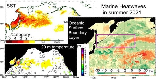
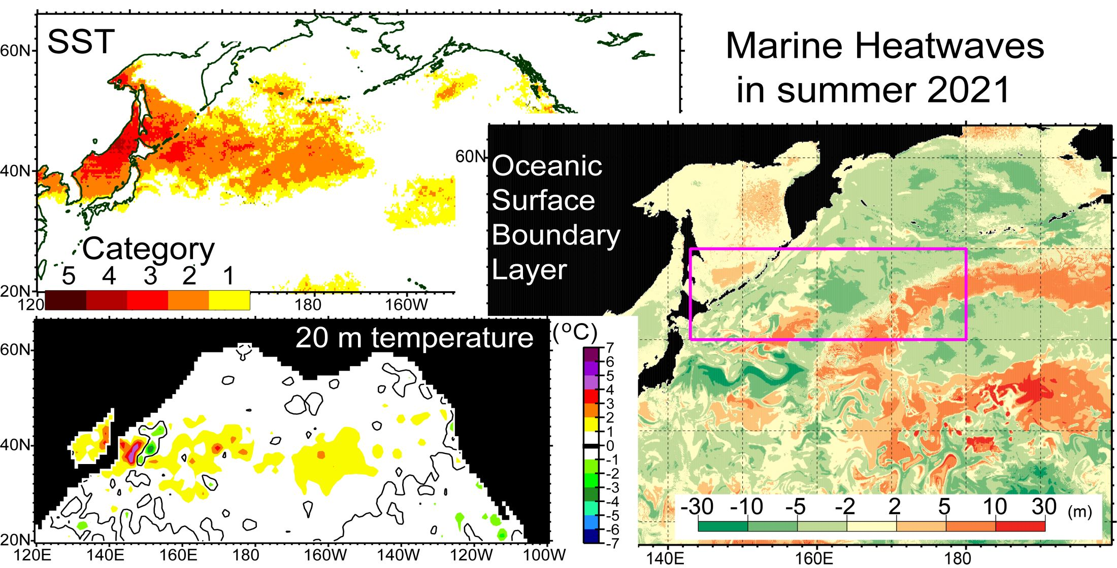
Figure 1a,b show intensity and age respectively, of MHWs on 30 July 2021, when the MHWs were at their maximum strength and extent, as explained later. The MHWs in the northwestern Pacific occurred within a zonal band, between 38°N and 50°N and extending from 120°E to 170°W, including the marginal seas, that is, the northern part of the Yellow Sea, the whole of the Sea of Japan, and the southern half of the Sea of Okhotsk. The MHW intensity on 30 July was classified into categories 1–4. Some areas of the MHWs corresponded to large SST anomalies > 6 °C (Figure 1d). The MHWs exhibited maximum intensity (i.e., category 4) on 30 July in the northern part of the Sea of Japan and tended to weaken gradually toward the east. The age of the MHWs in the northwestern Pacific on 30 July was within 1–30 days: it was longest (~30 days) in the northern part of the Sea of Japan and tended to be shorter further east.
It is worth noting that intense MHWs appeared to start on the northwestern shelf of the Sea of Okhotsk around 10 July 2021 and subsequently expand from there (Figure 1c,d). However, the SST data analyzed in this study did not strictly discriminate between SSTs in the presence or absence of sea ice; thus, if sea ice remained on the northwestern shelf at the beginning of summer, the estimated MHWs would include large uncertainties. Therefore, whether the above feature is a real phenomenon is questionable.
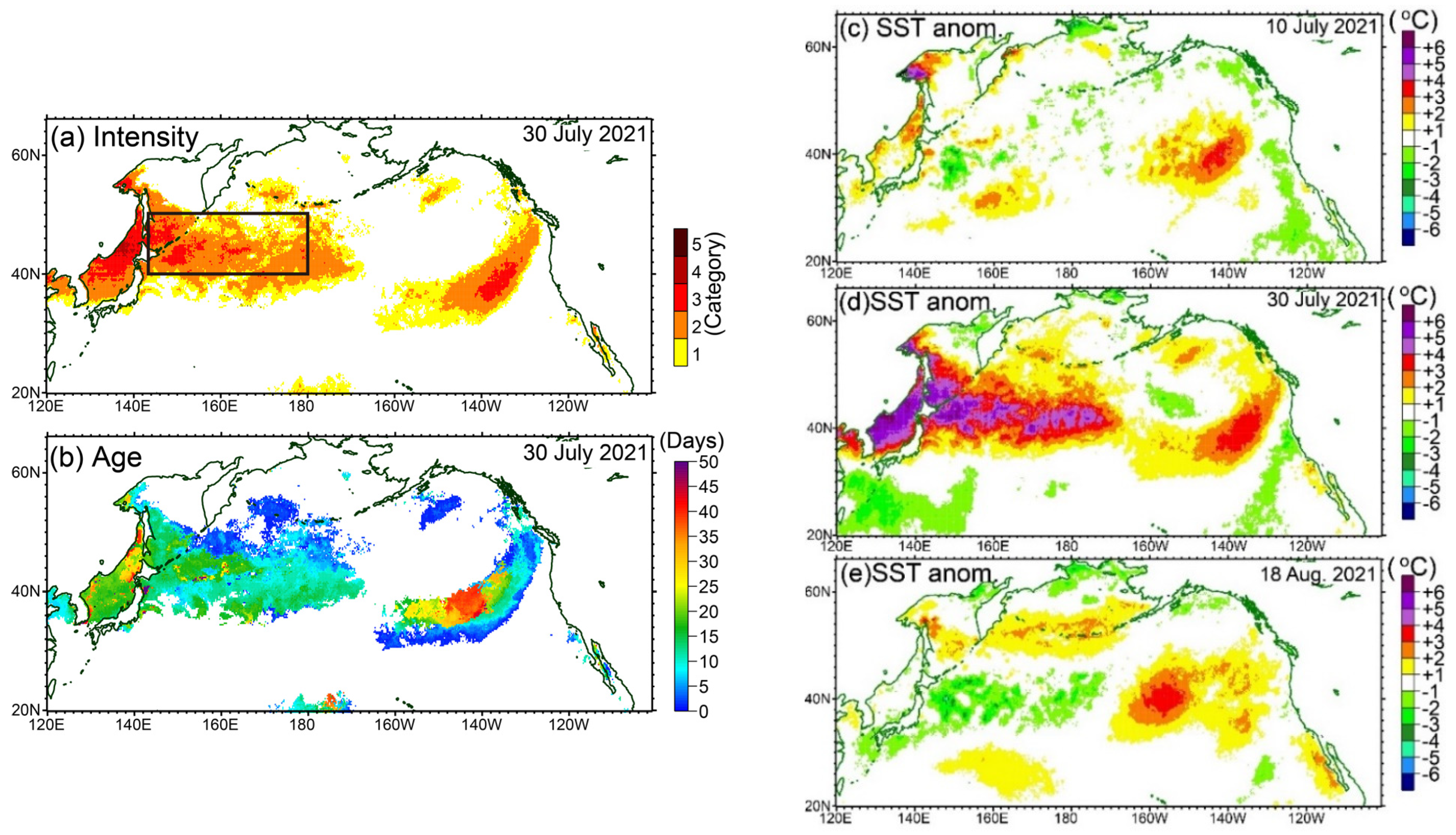
We focused on MHWs east of Japan in the northwestern Pacific and excluded from our analysis the Sea of Japan, where MHWs that were more intensive than those in 2021 occurred locally after 1982 (e.g., January 2020). Thus, we estimated daily time series of SST anomalies and the MHW index averaged over the rectangular area within 143°E–180° and 40°–50°N (Figure 2). Both time series show historical maxima in July–August 2021 (Figure 2a). The spatial mean of the daily MHW index exceeded 1.0 on a total of 207 days during 1982–2021, and 23 of these days were in July–August 2021. The spatial mean also exceeded 1.5 on 15 days during 1982–2021, of which 14 were in July–August 2021. These results indicate that the MHWs in summer 2021 were the most intense and extensive in the northwestern Pacific during the last four decades.
The transition to MHWs in summer 2021 can be interpreted as follows (Figure 2b). The MHWs started to develop on around 10 July 2021 (Figure 1c), when the spatial mean SST anomaly was close to zero (Figure 2b). The MHWs reached maximum intensity and extent around 30 July to 1 August (Figure 1d), and then immediately started to weaken. By 18 August (Figure 1e), the spatial mean SST anomaly was again near zero (Figure 2b) and the MHWs had almost entirely disappeared.
3.1.2. Heat Fluxes at the Sea Surface
Net heat flux anomalies at the sea surface during 10–30 July 2021 were mostly positive within the focal area, that is, the central area of MHWs (Figure 3a); thus, the sea surface was heated by the atmosphere, relative to the climatology. The distribution of net heat flux anomalies (Figure 3a) also correlated with that of SST anomaly differences between 10 and 30 July (Figure 3b) (r = 0.69), suggesting that the MHWs were attributable primarily to increased net heat fluxes at the sea surface over the northwestern Pacific.
The net heat fluxes were decomposed into four components: net shortwave radiation, net longwave radiation, latent heat, and sensible heat (Figure 4). Within our focal area, net shortwave radiation anomalies exhibited three positive maxima, centered around (145°E, 40°N), (170°E, 40°N), and (160°E, 45°N) (Figure 4b). These three positive maxima corresponded spatially to three negative minima of the total cloud cover and low cloud cover anomalies (see Section 3.3.1). Further, the spatial patterns of positive and negative net shortwave radiation anomalies in the focal area (Figure 4b) were roughly opposite to those of the other three components (Figure 4d,f,h), indicating that negative net shortwave radiation anomalies in the focal area were compensated by positive anomalies of the other three components. As a result, net heat flux anomalies at the sea surface were positive over the area of MHWs (Figure 3a).
Note that positive anomalies of net longwave radiation and sensible heat around the focal area (Figure 4d,h) corresponded to positive values of the respective components (Figure 4c,g). The positive values thus indicate that the sea surface was actually heated. Although MHWs with high SSTs were expected to cause large upward longwave radiation (i.e., negative heat fluxes), the net longwave radiation was nevertheless positive in some areas within the MHW area, for example, around the northwestern corner of the focal area (Figure 4c). This result suggests that strong downward longwave radiation from clouds exceeded the large upward longwave radiation from the sea surface. In fact, as described in Section 3.3.1, dense clouds tended to cover areas with positive net longwave radiation (Figure 4c). In any case, it should be emphasized that there were inter-regional differences in the origin of positive net heat flux anomalies over the area of MHWs; that is, the SST heating process differed inter-regionally within the area of MHWs.
3.2. Subsurface Ocean Conditions
3.2.1. Subsurface Sea Temperatures
In July 2021, temperatures in the subsurface at 20 m depth, just below the oceanic surface boundary layer, exhibited positive anomalies, mostly over the whole of the focal area (Figure 5c), although relatively large positive anomalies (>1 °C) were limited to its southern half. These relatively large positive anomalies were also distributed continuously after March 2021 (e.g., Figure 5a–c). In addition, subsurface temperatures at 20 m depth spatially averaged over the focal area reached a local maximum not in July 2021 but in May 2021 (Figure 5d), after which they decreased slightly until July 2021. Moreover, the positive anomalies in July 2021 were not the largest during 2004–2021. These features of the subsurface temperature were thus clearly different from the corresponding SST features. Hence, the main factors controlling the positive temperature anomalies in July 2021 seemed to differ between 20 m depth and the sea surface, and the MHWs that developed dramatically in summer 2021 were mostly limited to the sea surface (<20 m depth). With respect to this point, however, the positive subsurface temperature anomalies apparent after March 2021 might have contributed to the formation or maintenance of stratified conditions in the oceanic surface boundary layer in July 2021, as described in the next section.
3.2.2. Oceanic Surface Boundary Layer
In this study, the depth of the oceanic surface boundary layer, defined as the shallowest depth where the bulk Richardson number is equal to its critical value, was derived from model simulations instead of the more conventional mixed layer depth (i.e., the depth at which the water density in the upper layer exceeds a threshold value, typically 0.125 kg m−3, relative to the 10 m density), primarily because the mixed layer was very thin during summer 2021 and could not be accurately evaluated by the conventional mixed layer depth.
Hindcast and sensitivity experiments conducted with realistic ocean circulation models revealed that thickness anomalies of the oceanic surface boundary layer during 10–30 July 2021 were mainly negative within the focal area, except for an area of positive anomalies that extended southwest–northeast, from (165°E, 40°N) to (180°, 46°N) (Figure 6a). The thickness of the oceanic surface boundary layer remained small in the focal area during the period from 13 July to 5 August 2016 (Figure 6b), during most of which MHWs were rapidly developing (Figure 2b). From 7 August, however, the thickness increased abruptly, at the same time that the MHWs were weakening rapidly (Figure 2b). These results suggest that positive net heat fluxes (Figure 3a) and relatively weak wind stress (as explained in Section 3.3.1) near the sea surface stably maintained strong stratification, suppressed vertical convection, and accelerated the SST increase, that is, the rapid development of MHWs.
3.3. Atmospheric conditions
3.3.1. Conditions Near the Sea Surface
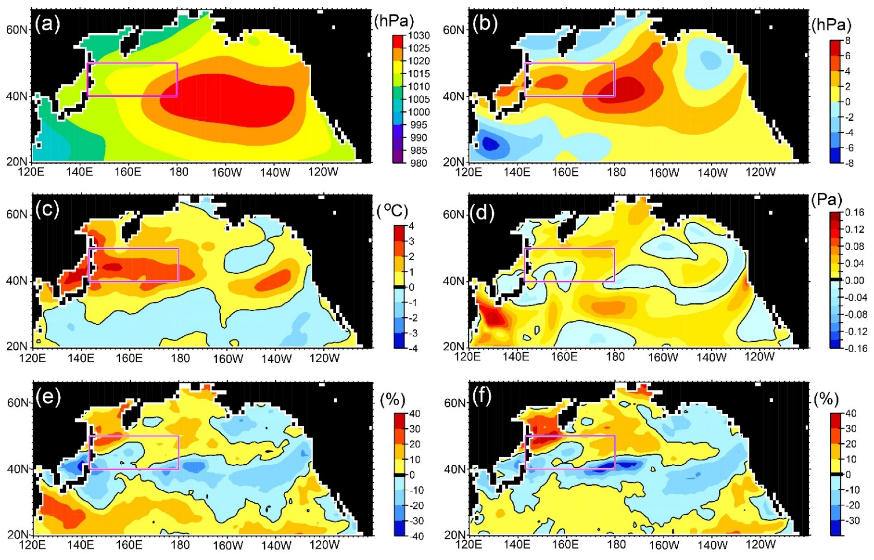
Sea level pressure anomalies during 10–30 July 2021 were widely positive in the northwestern Pacific, except in the northern Sea of Okhotsk and the western Bering Sea (Figure 7b). These positive anomalies were attributable to a northwestward expansion of the North Pacific Subtropical High (Figure 7a). The distribution of sea level pressure anomalies was also similar to MHW distribution (Figure 1a), although the distribution of air temperature anomalies near the sea surface (Figure 7c) more closely resembled the MHW distribution (Figure 1a). Local maxima of the air temperature anomalies exceeded 3 °C.
As mentioned in Section 3.1.2, the distributions of positive and negative anomalies of total and low cloud cover (Figure 7e,f) were almost opposite to those of positive and negative net shortwave radiation anomalies (Figure 4b). In addition, in the focal area, the positive anomalies of total and low cloud cover (Figure 7e,f) corresponded to both positive values and positive anomalies of net longwave radiation (Figure 4c,d), where strong downward longwave radiation from clouds to the sea surface exceeded the large upward longwave radiation attributed to MHWs. Moreover, as mentioned in Section 3.2.2, negative or small positive (<0.02 Pa) wind stress magnitude anomalies were distributed in the western half of the focal area (Figure 7d). In contrast, in the eastern half of the focal area, relatively large positive anomalies (0.02–0.06 Pa) were distributed in an area extending from southwest to northeast, corresponding to the area of positive oceanic surface boundary layer anomalies (Figure 6a).
3.3.2. Variation of the Westerly Jet at 200 hPa
Here, we focus on the westerly jet variation at 200 hPa as a potential driver or trigger of the atmospheric variations and MHWs in summer 2021. Maps of eastward wind velocity at 200 hPa averaged over 10–30 July (Figure 8a) revealed that the strong eastward wind (>20 m s−1) associated with the westerly jet [29] migrated northward, largely to the north of Japan, and skirted the focal area. The position of the velocity maximum reached 55°N at around 140°E. The velocity maximum between 120°E and 180° during 10–30 July 2021 was clearly located north of the climatological mean position (Figure 8b).
The northward shift of the westerly jet began suddenly at the beginning of July: large northward shifts of the westerly jet to the north of 50°N started at 70°E on 5 July, propagated eastward, and reached 120°–140°E around Japan on 11–15 July (Figure 9a). After 15 July, the meridional position of the jet in 143°E–180° stayed north of 50°N until the beginning of August, although it was intermittently disturbed (e.g., by typhoon events in late July): 50°N corresponded to the northern boundary of the MHWs in the northwestern Pacific (Figure 1a). After around 1–8 August, the axial position of the jet was displaced to the south. Simultaneously, the MHWs in the northwestern Pacific started to weaken and shrink.
The large northward shift of the westerly jet identified in early to mid-July exceeded the climatological mean plus 3 standard deviations (Figure 9b); therefore, it was interpreted as a rare event. This result suggests that the abnormally large northward shift of the westerly jet triggered warm atmospheric conditions near the sea surface and thus caused the strongest, most extensive MHWs yet recorded over the northwestern Pacific.
4. Discussion
In this article, we reported on the most extensive and intense MHWs in the historical record of the last 40 years, which occurred in the northwestern Pacific during July–August 2021. However, we mainly limited our explanation to certain features: SST, the oceanic surface boundary layer, heat flux at the sea surface, and atmospheric conditions. We only briefly mentioned the redistribution of heat from the sea surface to the ocean subsurface by ocean advection and diffusion. In addition, although differences in SST anomalies were positively correlated with net heat flux anomalies (r = 0.69, Figure 3), anomalies of SST and net heat flux were not strongly correlated with each other. In considering these problems, the uncertainties of the SST and heat flux data should first of all be meticulously validated by comparing different datasets with each other and with in situ data (e.g., surface buoy and vessel data). Moreover, it should be noted that the core area of the MHWs was at 43°–46°N (not shown), whereas the net heat flux anomalies did not show corresponding maxima at 43°–46°N. Additionally, as described in Section 3.1.2, SST heating processes differed inter-regionally within the area of MHWs. Hence, we anticipate that a feedback process from the ocean to the atmosphere contributed to localized enhancement of MHWs. Air–sea processes that might be involved in the enhancement of MHWs at mid-latitudes include SST–cloud feedback (e.g., [30,31,32]), surface heat flux feedback dominated by turbulent flux (e.g., [33]), or an air–sea process related to the imbalance between incoming and outgoing fluxes through the sea surface (e.g., [34]). A useful first step to clarify such processes would be to conduct numerical experiments with a coupled air–sea model.
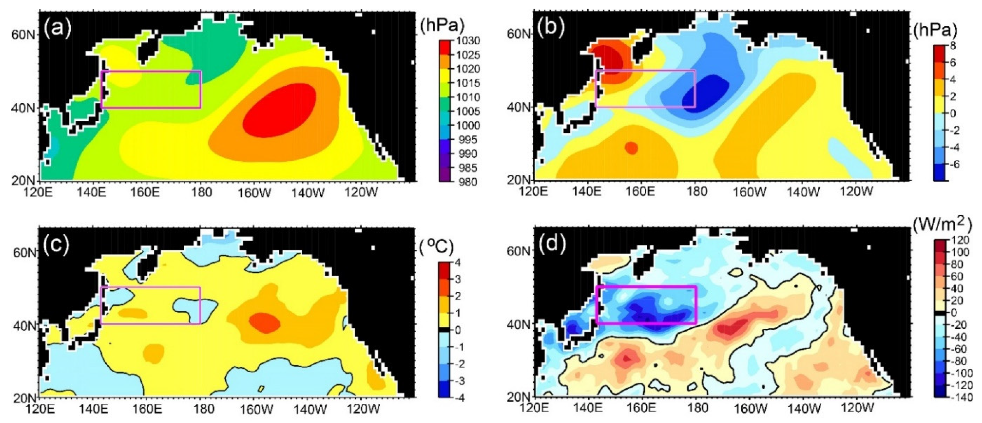
In this article, we also focused mainly on the development of MHWs in the northwestern Pacific, but the MHWs also decayed rapidly after the westerly jet was displaced southward at the beginning of August 2021. Therefore, we provide here a brief description of atmospheric conditions near the sea surface during 1–18 August 2021. In this period, the North Pacific Subtropical High retreated southward, and the Okhotsk High strengthened (Figure 10a). The sea level pressure valley between the two high-pressure systems was located in the southeastern half of the focal area (143°E–180°, 40°–50°N) (Figure 10a,b). Air temperature greatly decreased over the northwestern Pacific after 1 August (Figure 10c), and the negative net heat flux anomalies at the sea surface in the focal area (Figure 10d) contributed to sea surface cooling. Simultaneously, as shown by hindcast experiments, the oceanic surface boundary layer deepened (Figure 6b), and this deepening implies that entrainment of subsurface water into the surface boundary layer accelerated cooling at the sea surface. As a consequence, the extensive and intense MHWs had disappeared by 18 August.
5. Conclusions
In July–August 2021, the largest and most intense MHWs of the satellite era occurred at the sea surface over extensive areas of the northwestern Pacific Ocean. These were observed at the sea surface and were accompanied by a stable shallow oceanic surface boundary layer. Their spatial relationship to heat fluxes at the sea surface indicates that the MHWs were generated mainly by atmospheric forcing associated with northwestward expansion of the North Pacific Subtropical High and northward displacement of the westerly jet. Additional air–sea studies are needed to understand inter-regional differences in SST heating processes within the area of MHWs.
Moreover, the MHWs in summer 2021 were limited to the vicinity of the sea surface (<20 m depth), where primary production is especially high (e.g., [35,36,37]). In fact, some studies have reported impacts of MHWs on lower trophic levels of marine ecosystems (e.g., [38,39]). Commercially important fisheries’ resources include Japanese sardine Sardinops melanostictus and Pacific saury Cololabis saira, which utilize the northwestern Pacific waters around the focal area as a nursery ground in summer (e.g., [40,41]). Hence, for sustainable management of ecosystems in the northwestern Pacific Ocean, physical and biological studies are essential, not only to evaluate influences of the 2021 MHWs but also to project the influences of future MHWs on marine ecosystems.
Author Contributions
Conceptualization, H.K.; methodology, H.K. and T.S.; software, H.K. and T.S.; validation, H.K and T.S.; investigation, H.K.; writing—original draft preparation, H.K.; writing—review and editing, T.S.; visualization, H.K.; funding acquisition, H.K. All authors have read and agreed to the published version of the manuscript.
Funding
This research was supported by KAKENHI, Grant Number 19K06216, from the Ministry of Education, Culture, Sports, Science and Technology, and by the Environment Research and Technology Development Fund (4-2102) of the Environmental Restoration and Conservation Agency of Japan. This work was also partially supported by the Fisheries Agency (promotion project to precisely estimate fish stock size around Japan (no grant number)), but the contents of this study do not necessarily reflect the views of the Fisheries Agency.
Data Availability Statement
All the data analyzed in this study are publicly available. SST data were collected from a data server of NEAR-GOOS (https://ds.data.jma.go.jp) (accessed on 2 September 2021). JRA-55 data were downloaded from the University Corporation for Atmospheric Research data server (https://rda.ucar.edu) (accessed on 4 September 2021). Gridded Argo-based seawater temperatures in the subsurface were obtained from Scripps Institute of Oceanography (http://sio-argo.ucsd.edu/RG_Climatology.html) (accessed on 17 August 2021). Daily reanalysis data from FRA-ROMS are available at http://fm.dc.affrc.go.jp/fra-roms after user registration (accessed on 15 August 2021). The source code of the ocean circulation models based on Rutgers University’s ROMS is available at https://www.myroms.org (accessed on 15 August 2021).
Acknowledgments
Numerical experiments based on FRA-ROMS were conducted using the Scientific Computing System in the Agriculture, Forestry and Fisheries Research Information Technology Center. We extend a special thanks to associate editors, special issue editors, and three reviewers for many constructive and fruitful comments.
Conflicts of Interest
The authors declare no conflict of interest.
References
- Seneviratne, S.I.; Nicholls, N.; Easterling, D.; Goodess, C.M.; Kanae, S.; Kossin, J.; Luo, Y.; Marengo, J.; McInnes, K.; Rahimi, M.; et al. Changes in Climate Extremes and their Impacts on the Natural Physical Environment. In Managing the Risks of Extreme Events and Disasters to Advance Climate Change Adaptation, 1st ed.; Field, C.B., Barros, V., Stocker, T.F., Qin, D., Dokken, D.J., Ebi, K.L., Mastrandrea, M.D., Mach, K.J., Plattner, G.-K., Allen, S.K., et al., Eds.; A Special Report of Working Groups I and II of the Intergovernmental Panel on Climate Change (IPCC); Cambridge University Press: Cambridge, UK; New York, NY, USA, 2012; pp. 109–230. Available online: https://www.ipcc.ch/site/assets/uploads/2018/03/SREX-Chap3_FINAL-1.pdf (accessed on 5 September 2021).
- Fischer, E.M.; Knutti, R. Anthropogenic contribution to global occurrence of heavy-precipitation and high-temperature extremes. Nat. Clim. Chang. 2015, 5, 560–564. [Google Scholar] [CrossRef]
- Easterling, D.R.; Kunkel, K.E.; Wehner, M.F.; Sun, L. Detection and attribution of climate extremes in the observed record. Weather. Clim. Extrem. 2016, 11, 17–27. [Google Scholar] [CrossRef] [Green Version]
- Mitchell, J.F.B.; Lowe, J.; Wood, R.A.; Vellinga, M. Extreme events due to human-induced climate change. Phil. Trans. R. Soc. A 2006, 364, 2117–2133. [Google Scholar] [CrossRef]
- Hobday, A.J.; Alexander, L.V.; Perkins, S.E.; Smale, D.A.; Straub, S.C.; Oliver, E.C.J.; Benthuysen, J.A.; Burrows, M.T.; Donat, M.G.; Feng, M.; et al. A hierarchical approach to defining marine heatwaves. Prog. Oceanogr. 2016, 141, 227–238. [Google Scholar] [CrossRef] [Green Version]
- Hobday, A.J.; Oliver, E.C.J.; Sen Gupta, A.; Benthuysen, J.A.; Burrows, M.T.; Donat, M.G.; Holbrook, N.J.; Moore, P.J.; Thomsen, M.S.; Wernberg, T.; et al. Categorizing and naming marine heatwaves. Oceanography 2018, 31, 162–173. [Google Scholar] [CrossRef] [Green Version]
- Holbrook, N.J.; Scannell, H.A.; Sen Gupta, A.; Benthuysen, J.A.; Feng, M.; Oliver, E.C.J.; Alexander, L.V.; Burrows, M.T.; Donat, M.G.; Hobday, A.J.; et al. A global assessment of marine heatwaves and their drivers. Nat. Commun. 2019, 10, 2624. [Google Scholar] [CrossRef]
- Oliver, E.C.J.; Donat, M.G.; Burrows, M.T.; Moore, P.J.; Smale, D.A.; Alexander, L.V.; Benthuysen, J.A.; Feng, M.; Sen Gupta, A.; Hobday, A.J.; et al. Longer and more frequent marine heatwaves over the past century. Nat. Commun. 2018, 9, 1324. [Google Scholar] [CrossRef]
- Oliver, E.C.J. Mean warming not variability drives marine heatwave trends. Clim. Dyn. 2019, 53, 1653–1659. [Google Scholar] [CrossRef]
- Oliver, E.C.J.; Burrows, M.T.; Donat, M.G.; Sen Gupta, A.; Alexander, L.V.; Perkins-Kirkpatrick, S.E.; Benthuysen, J.A.; Hobday, A.J.; Holbrook, N.J.; Moore, P.J.; et al. Projected marine heatwaves in the 21st century and the potential for ecological impact. Front. Mar. Sci. 2019, 6, 734. [Google Scholar] [CrossRef] [Green Version]
- Straub, S.C.; Wernberg, T.; Thomsen, M.S.; Moore, P.J.; Burrows, M.T.; Harvey, B.P.; Smale, D.A. Resistance, extinction, and everything in between—The diverse responses of seaweeds to marine heatwaves. Front. Mar. Sci. 2019, 6, 763. [Google Scholar] [CrossRef]
- Jacox, M.G.; Alexander, M.A.; Bograd, S.J.; Scott, J.D. Thermal displacement by marine heatwaves. Nature 2020, 584, 82–86. [Google Scholar] [CrossRef] [PubMed]
- Piatt, J.F.; Parrish, J.K.; Renner, H.M.; Schoen, S.K.; Jones, T.T.; Arimitsu, M.L.; Kuletz, K.J.; Bodenstein, B.; García-Reyes, M.; Duerr, R.S.; et al. Extreme mortality and reproductive failure of common murres resulting from the northeast Pacific marine heatwave of 2014-2016. PLoS ONE 2020, 15, e0226087. [Google Scholar] [CrossRef] [Green Version]
- Cheung, W.W.L.; Frölicher, T.L. Marine heatwaves exacerbate climate change impacts for fisheries in the northeast Pacific. Sci. Rep. 2020, 10, 6678. [Google Scholar] [CrossRef]
- Gómez-Gras, D.; Linares, C.; Dornelas, M.; Madin, J.S.; Brambilla, V.; Ledoux, J.-B.; López-Sendino, P.; Bensoussan, N.; Garrabou, J. Climate change transforms the functional identity of Mediterranean coralligenous assemblages. Ecol. Lett. 2021, 24, 1038–1051. [Google Scholar] [CrossRef]
- Di Lorenzo, E.; Mantua, N. Multi-year persistence of the 2014/15 North Pacific marine heatwave. Nat. Clim. Chang. 2016, 6, 1042–1047. [Google Scholar] [CrossRef]
- Hayashi, M.; Shiogama, H.; Emori, S.; Ogura, T.; Hirota, N. The northwestern Pacific warming record in August 2020 occurred under anthropogenic forcing. Geophys. Res. Lett. 2021, e2020GL090956. [Google Scholar] [CrossRef]
- Miyama, T.; Minobe, S.; Goto, H. Marine heatwave of sea surface temperature of the Oyashio region in summer in 2010–2016. Front. Mar. Sci. 2021, 7, 576240. [Google Scholar] [CrossRef]
- Kuroda, H.; Taniuchi, Y.; Kasai, H.; Nakanowatari, T.; Setou, T. Co-occurrence of marine extremes induced by tropical storms and an ocean eddy in summer 2016: Anomalous hydrographic conditions in the Pacific shelf waters off southeast Hokkaido, Japan. Atmosphere 2021, 12, 888. [Google Scholar] [CrossRef]
- Kuroda, H.; Yokouchi, K. Interdecadal decrease in potential fishing areas for Pacific saury off the southeastern coast of Hokkaido, Japan. Fish. Oceanogr. 2017, 26, 439–454. [Google Scholar] [CrossRef]
- Kurihara, Y.; Sakurai, T.; Kuragano, T. Global daily sea surface temperature analysis using data from satellite microwave radiometer, satellite infrared radiometer and in-situ observations. Weather. Serv. Bull. 2006, 73, S1–S18. (In Japanese) [Google Scholar]
- Roemmich, D.; Gilson, J. The 2004-2008 mean and annual cycle of temperature, salinity, and steric height in the global ocean from the Argo Program. Prog. Oceanogr. 2009, 82, 81–100. [Google Scholar] [CrossRef]
- Kobayashi, S.; Ota, Y.; Harada, Y.; Ebita, A.; Moriya, M.; Onoda, H.; Onogi, K.; Kamahori, H.; Kobayashi, C.; Endo, H.; et al. The JRA-55 reanalysis: General specifications and basic characteristics. J. Meteor. Soc. Jpn. 2016, 93, 5–48. [Google Scholar] [CrossRef] [Green Version]
- Kuroda, H.; Setou, T.; Kakehi, S.; Ito, S.; Taneda, T.; Azumaya, T.; Inagake, D.; Hiroe, Y.; Morinaga, K.; Okazaki, M.; et al. Recent advances in Japanese fisheries science in the Kuroshio-Oyashio region through development of the FRA-ROMS ocean forecast system: Overview of the reproducibility of reanalysis products. Open J. Mar. Sci. 2017, 7, 62–90. [Google Scholar] [CrossRef] [Green Version]
- Shchepetkin, A.F.; McWilliams, J.C. A method for computing horizontal pressure-gradient force in an oceanic model with a nonaligned vertical coordinate. J. Geophys. Res. 2003, 108, 3090. [Google Scholar] [CrossRef]
- Shchepetkin, A.F.; McWilliams, J.C. The regional oceanic modeling system (ROMS): A split-explicit, free-surface, topography-following-coordinate oceanic model. Ocean Modell. 2005, 9, 347–404. [Google Scholar] [CrossRef]
- Haidvogel, D.B.; Arango, H.; Budgell, W.P.; Cornuelle, B.D.; Curchitser, E.; Di Lorenzo, E.; Fennel, K.; Geyer, W.R.; Hermann, A.J.; Lanerolle, L.; et al. Ocean forecasting in terrain-following coordinates: Formulation and skill assessment of the Regional Ocean Modeling System. J. Comput. Phys. 2008, 227, 3595–3624. [Google Scholar] [CrossRef]
- Kuroda, H.; Setou, T.; Aoki, K.; Takahashi, D.; Shimizu, M.; Watanabe, T. A numerical study of the Kuroshio-induced circulation in Tosa Bay, off the southern coast of Japan. Cont. Shelf Res. 2013, 53, 50–62. [Google Scholar] [CrossRef]
- Schiemann, R.; Lüthi, D.; Schär, C. Seasonality and interannual variability of the westerly jet in the Tibetan Plateau region. J. Clim. 2009, 22, 2940–2957. [Google Scholar] [CrossRef]
- Clement, A.M.; Burgman, R.; Norris, J.R. Observational and model evidence for positive low-level cloud feedback. Science 2009, 325, 460–464. [Google Scholar] [CrossRef] [Green Version]
- Wu, R.; Kinter, J.L. Atmosphere-ocean relationship in the midlatitude North Pacific: Seasonal dependence and east-west contrast. J. Geophys. Res. 2010, 115, D06101. [Google Scholar] [CrossRef]
- Schmeisser, L.; Bond, N.A.; Siedlecki, S.A.; Ackerman, T.P. The role of clouds and surface heat fluxes in the maintenance of the 2013–2016 Northeast Pacific marine heatwave. J. Geophys. Res. Atmos. 2019, 124, 10772–10783. [Google Scholar] [CrossRef]
- Frankignoul, C.; Kestenare, E. The surface heat flux feedback. Part I: Estimates from observations in the Atlantic and the North Pacific. Clim. Dyn. 2002, 19, 633–647. [Google Scholar] [CrossRef]
- Pinault, J.-L. Modulated response of subtropical gyres: Positive feedback loop, subharmonic modes, resonant solar and orbital forcing. J. Mar. Sci. Eng. 2018, 6, 107. [Google Scholar] [CrossRef] [Green Version]
- Shiomoto, A.; Sasaki, K.; Shimoda, T.; Matsumura, S. Primary Productivity in the Offshore Oyashio in the Spring and Summer 1990. J. Oceanogr. 1994, 50, 209–222. [Google Scholar] [CrossRef]
- Shiomoto, A.; Ishida, Y.; Tamaki, T.; Yamanaka, Y. Primary production and chlorophyll a in the northwestern Pacific Ocean in summer. J. Geophys. Res. 1998, 103, 24651–24661. [Google Scholar] [CrossRef]
- Kameda, T.; Matsumura, S. Chlorophyll biomass off Sanriku, northwestern Pacific estimated by Ocean Color and Temperature Scanner (OCTS) and a vertical distribution model. J. Oceanogr. 1998, 54, 509–516. [Google Scholar] [CrossRef]
- Hayashida, H.; Matear, R.J.; Strutton, P.G. Background nutrient concentration determines phytoplankton bloom response to marine heatwaves. Glob Change Biol. 2020, 26, 4800–4811. [Google Scholar] [CrossRef] [PubMed]
- Montie, S.; Thomsen, M.; Rack, W.; Broady, P. Extreme summer marine heatwaves increase chlorophyll a in the Southern Ocean. Antarct. Sci. 2020, 32, 508–509. [Google Scholar] [CrossRef]
- Okunishi, T.; Ito, S.; Ambe, D.; Takasuka, A.; Kameda, T.; Tadokoro, K.; Setou, T.; Komatsu, K.; Kawabata, A.; Kubota, H.; et al. A modeling approach to evaluate growth and movement for recruitment success of Japanese sardine (Sardinops melanostictus) in the western Pacific. Fish. Oceanogr. 2012, 21, 44–57. [Google Scholar] [CrossRef]
- Miyamoto, H.; Vijai, D.; Kidokoro, H.; Tadokoro, K.; Watanabe, T.; Fuji, T.; Suyama, S. Geographic variation in feeding of Pacific saury Cololabis saira in June and July in the North Pacific Ocean. Fish. Oceanogr. 2020, 29, 558–571. [Google Scholar] [CrossRef]
Figure 1.
(a) Intensity and (b) age of marine heatwaves (MHWs) on 30 July 2021. In (a), the rectangle indicates the area within 143°E–180° and 40°–50°N, the focal area of our analysis. SST anomalies are shown on (c) 10 July, (d) 30 July, and (e) 18 August 2021.
Figure 1.
(a) Intensity and (b) age of marine heatwaves (MHWs) on 30 July 2021. In (a), the rectangle indicates the area within 143°E–180° and 40°–50°N, the focal area of our analysis. SST anomalies are shown on (c) 10 July, (d) 30 July, and (e) 18 August 2021.

Figure 2.
Time series of the daily SST anomaly (blue lines, corresponding to the right blue axes) and MHW index (red lines, corresponding to the left red axes) during (a) 1982–2021 and (b) June–August 2021. The SST anomaly and MHW index were estimated at each grid point and then spatially averaged over 143°E–180° and 40°–50°N (rectangle in Figure 1a). As indices for evaluating the variability of the daily SST anomaly, the +3 standard deviation line (dashed blue line) is shown in (a), and the daily SST anomaly normalized by the standard deviation at each grid point and spatially averaged over the focal area (green line, corresponding to the right green axis) is shown in (b).

Figure 3.
(a) Net heat flux anomalies (Qnet′) at the sea surface during 10–30 July 2021. (b) SST anomaly differences between 10 and 30 July 2021 (ΔSST′). The pink rectangle indicates the focal area (143°E–180°, 40°–50°N).
Figure 3.
(a) Net heat flux anomalies (Qnet′) at the sea surface during 10–30 July 2021. (b) SST anomaly differences between 10 and 30 July 2021 (ΔSST′). The pink rectangle indicates the focal area (143°E–180°, 40°–50°N).
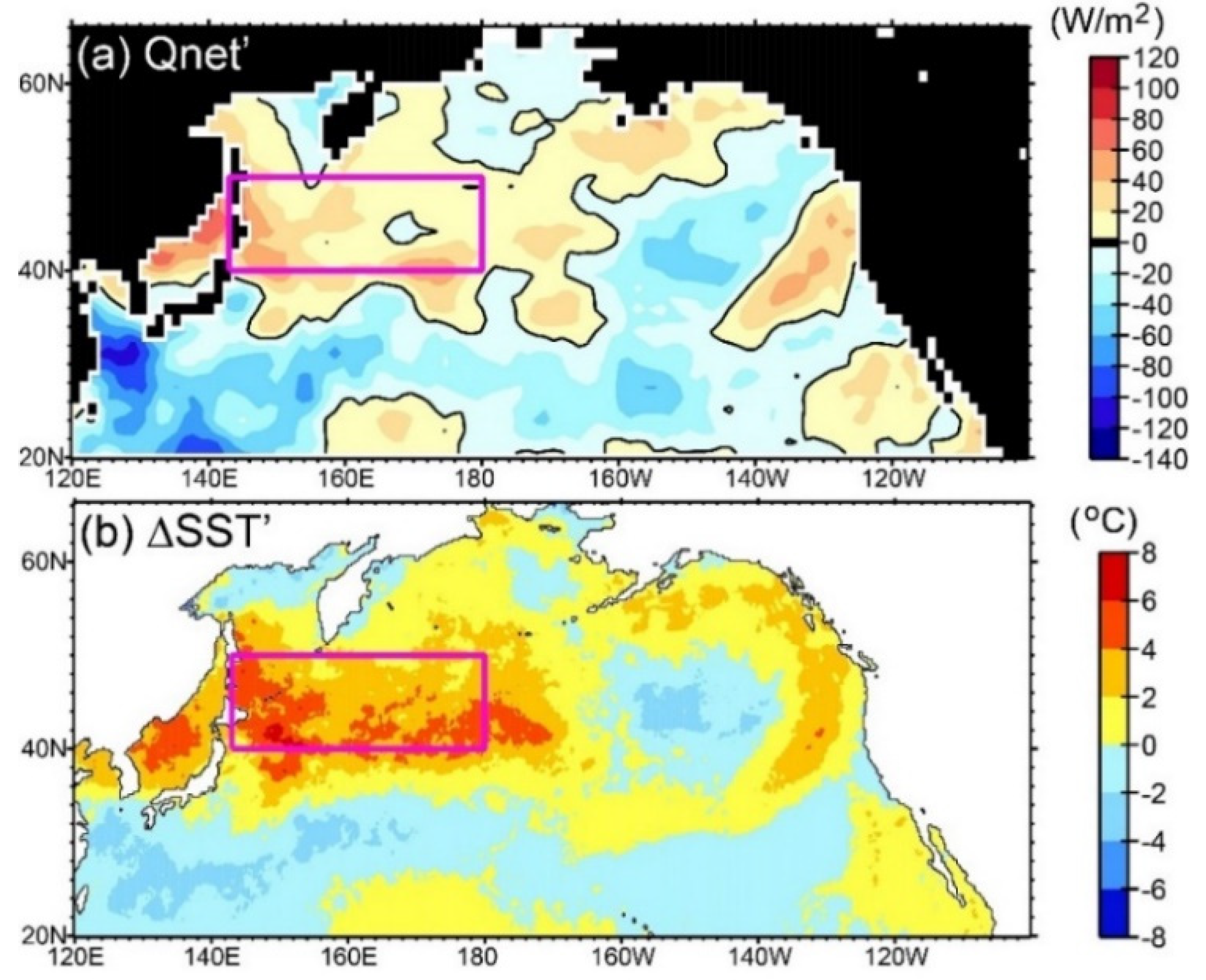
Figure 4.
(a) Net shortwave radiation, (c) net longwave radiation, (e) latent heat, and (g) sensible heat flux averaged over 10–30 July 2021. Anomalies of (b) net shortwave radiation, (d) net longwave radiation, (f) latent heat, and (h) sensible heat flux.
Figure 4.
(a) Net shortwave radiation, (c) net longwave radiation, (e) latent heat, and (g) sensible heat flux averaged over 10–30 July 2021. Anomalies of (b) net shortwave radiation, (d) net longwave radiation, (f) latent heat, and (h) sensible heat flux.
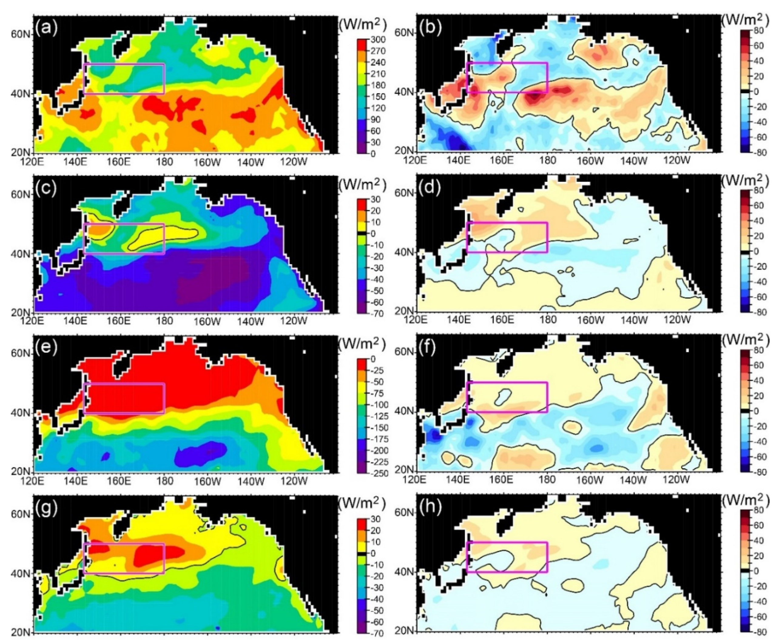
Figure 5.
Monthly seawater temperature anomalies at 20 m below the sea surface in (a) May, (b) June, and (c) July 2021. (d) Monthly time series of the temperature anomalies averaged over the focal area (143°E–180°, 40°–50°N). In (d), the scale of the horizontal axis for the year 2021 has been enlarged. The monthly subsurface temperature anomalies in 2021 are depicted by closed circles connected by a bold line.
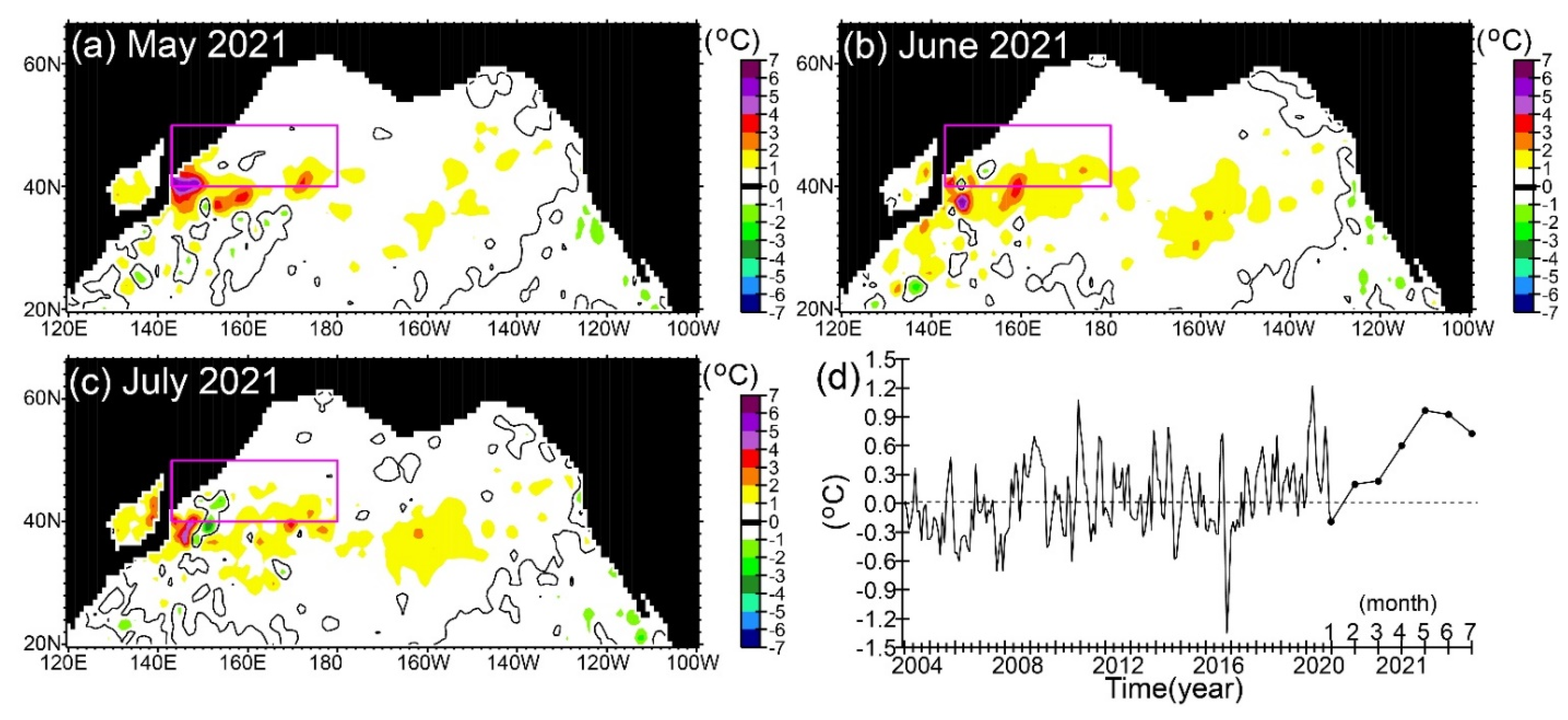
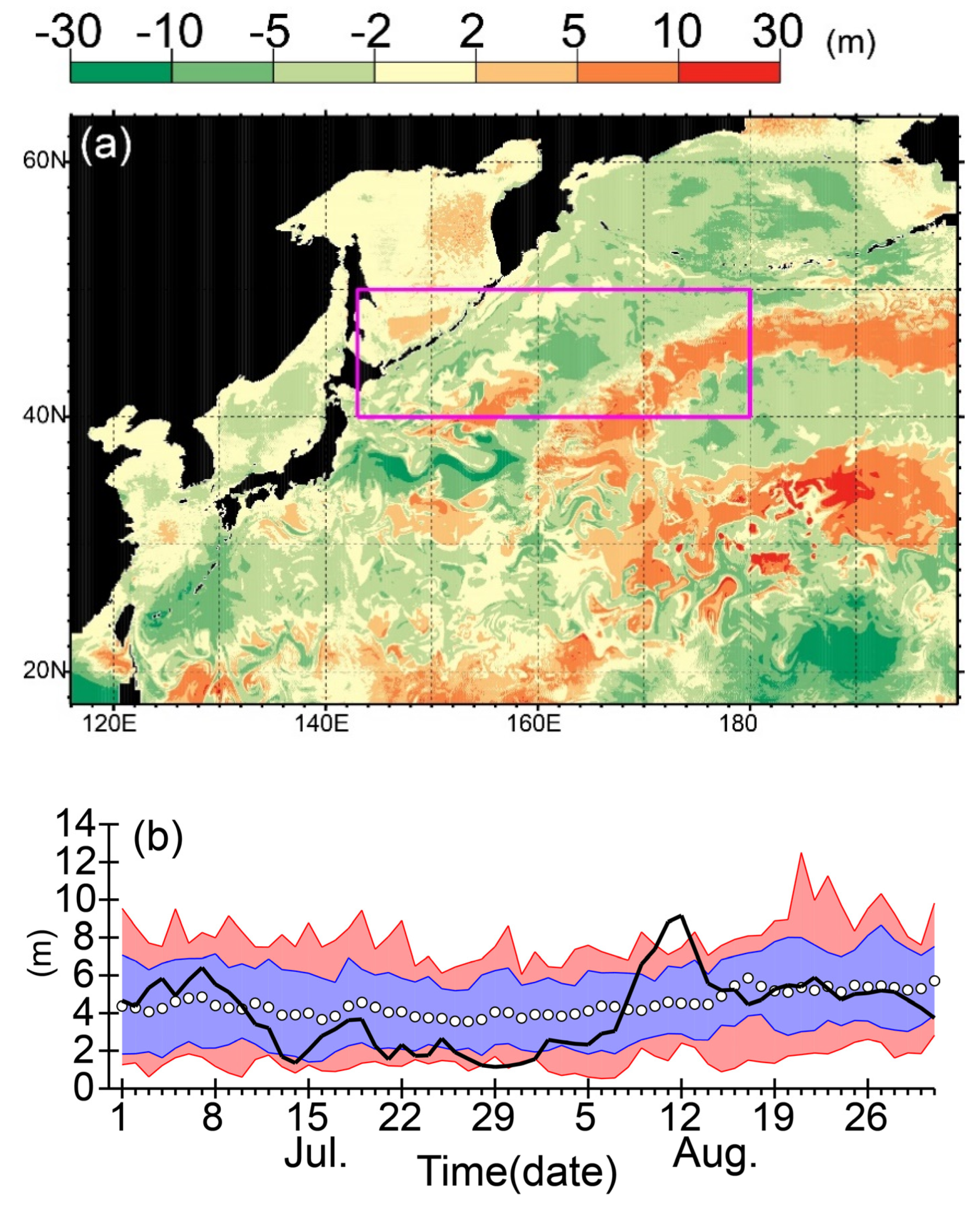
Figure 6.
(a) Thickness anomalies of the oceanic surface boundary layer during 10–30 July 2021, estimated by a mixed layer model based on K-profile parameterization in the 1/10° ocean circulation model. Climatological means were estimated by averaging the thickness over 30 sensitivity simulations based on external forcings in 1990–2019. (b) Time series of oceanic surface boundary layer thickness spatially averaged over the focal area (143°E–180° and 40°–50°N; the purple rectangle in (a)). The bold black line shows the daily time series in 2021. Open circles denote daily means of the 30 simulations. Blue shading shows the 10th to 90th percentile range. Red shading shows the range, beyond these percentiles, between the minimum and maximum.

Figure 7.
(a) Sea level pressure during 10–30 July 2021. Anomalies during 10–30 July 2021: (b) sea level pressure, (c) air temperature at 2 m above the sea surface, (d) magnitude of wind stress at 10 m above the sea surface, (e) total cloud cover, and (f) low cloud cover.
Figure 7.
(a) Sea level pressure during 10–30 July 2021. Anomalies during 10–30 July 2021: (b) sea level pressure, (c) air temperature at 2 m above the sea surface, (d) magnitude of wind stress at 10 m above the sea surface, (e) total cloud cover, and (f) low cloud cover.

Figure 8.
Eastward wind velocity at 200 hPa averaged over 10–30 July (a) in 2021 and (b) 1990–2019. The purple rectangle indicates the focal area (143°E–180°, 40°–50°N). Strong velocities of >20 m s−1 are associated with the westerly jet.
Figure 8.
Eastward wind velocity at 200 hPa averaged over 10–30 July (a) in 2021 and (b) 1990–2019. The purple rectangle indicates the focal area (143°E–180°, 40°–50°N). Strong velocities of >20 m s−1 are associated with the westerly jet.
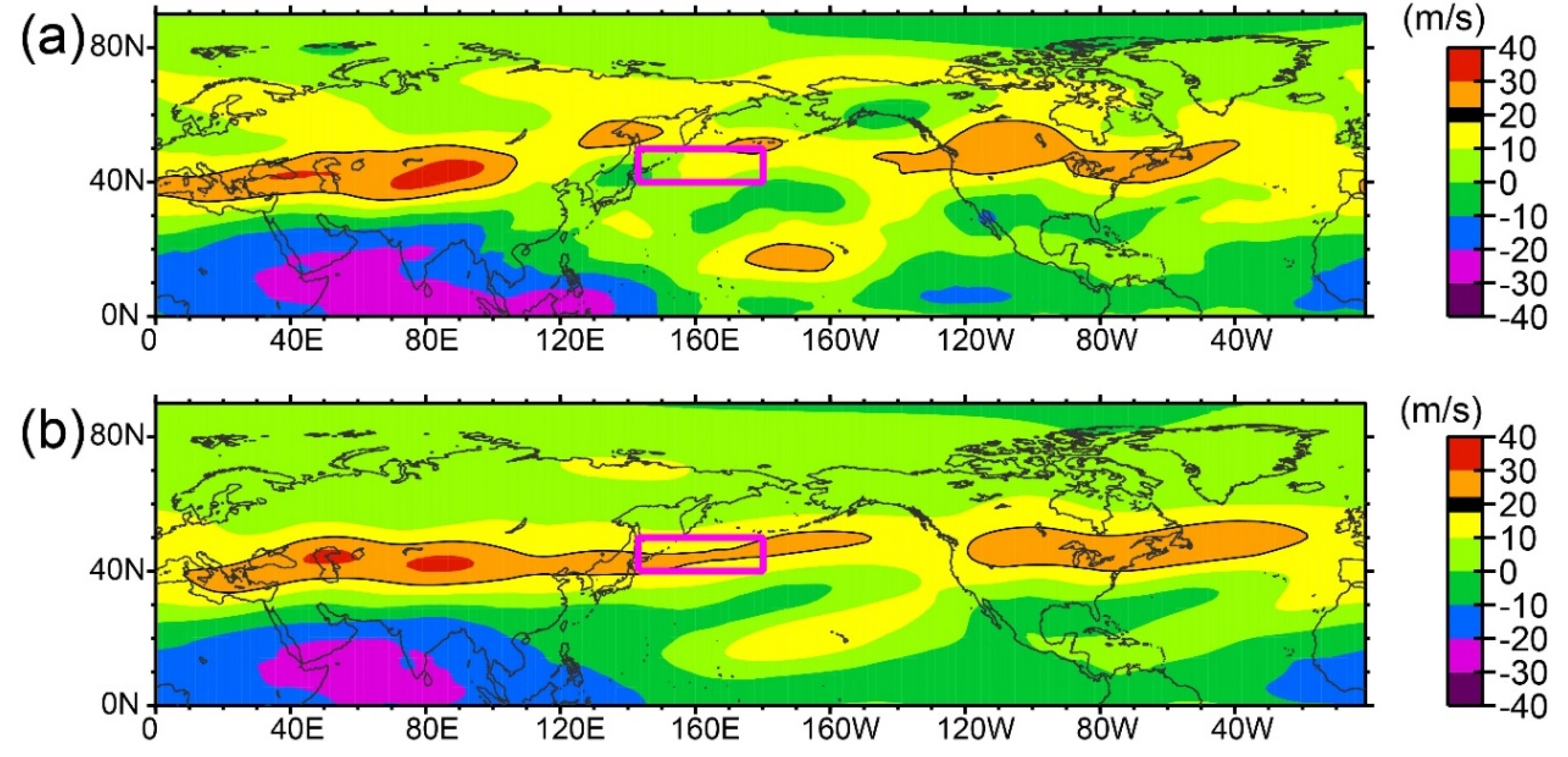
Figure 9.
(a) Daily meridional position of the westerly jet axis during June–August 2021. The jet axis was defined as the velocity maximum at 200 hPa between 30°N and 60°N. When the velocity maximum was at either 30°N or 60°N, the axis position was not specified (i.e., white areas). (b) Normalized anomalies of the axis position. The daily mean axis position (Y) was normalized by the 30-year daily mean (M) and the standard deviation (S): i.e., (Y – M)/S. The values of 50°N in panel (a) and 3 in panel (b) are emphasized by bold contours. The red dashed rectangle denotes the area within 143°E–180°.
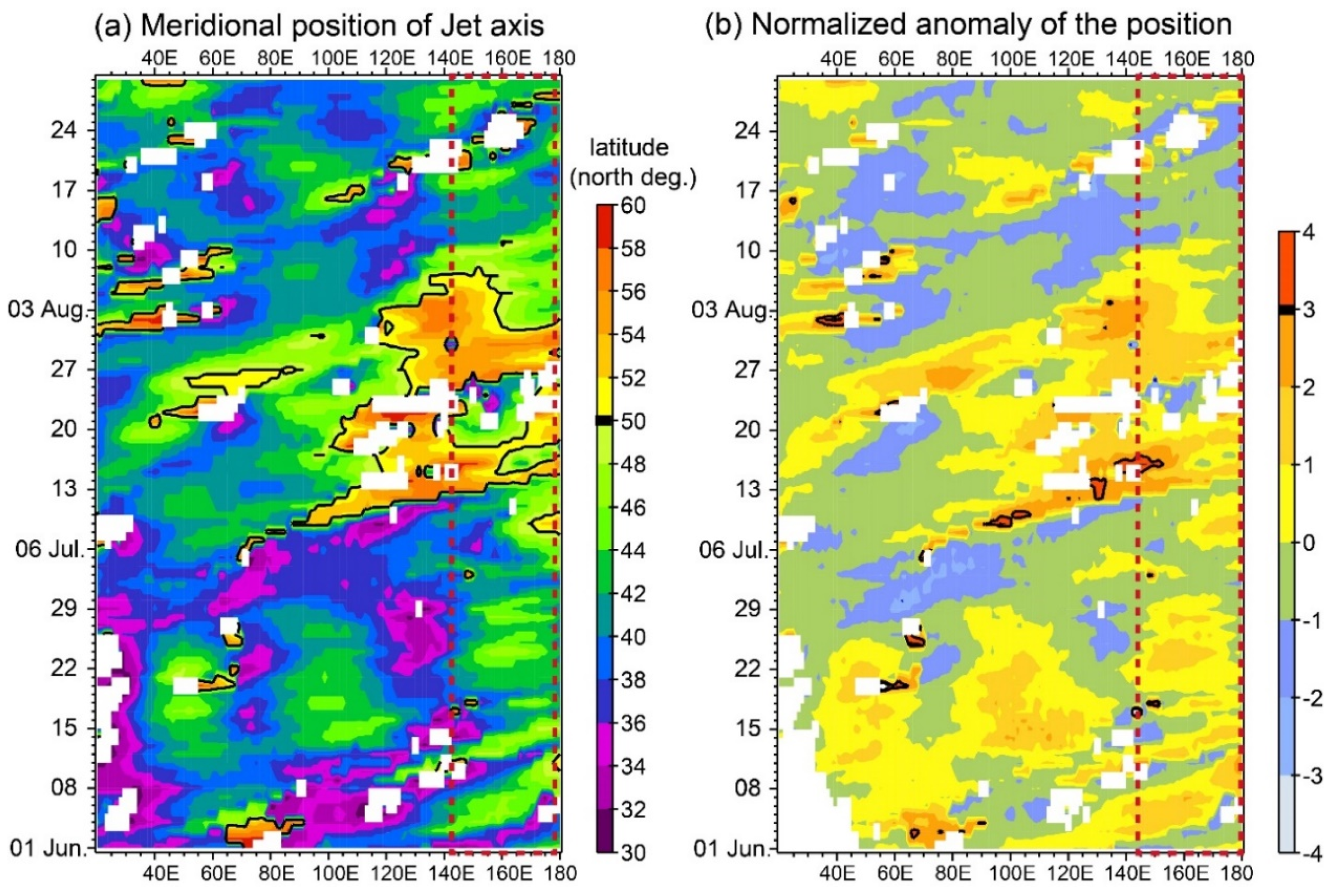
Figure 10.
(a) Sea level pressure during 1–18 August 2021. Anomalies during the same period: (b) sea level pressure, (c) air temperature at 2 m above the sea surface, and (d) net heat flux at the sea surface.
Figure 10.
(a) Sea level pressure during 1–18 August 2021. Anomalies during the same period: (b) sea level pressure, (c) air temperature at 2 m above the sea surface, and (d) net heat flux at the sea surface.
Publisher’s Note: MDPI stays neutral with regard to jurisdictional claims in published maps and institutional affiliations. |
© 2021 by the authors. Licensee MDPI, Basel, Switzerland. This article is an open access article distributed under the terms and conditions of the Creative Commons Attribution (CC BY) license (https://creativecommons.org/licenses/by/4.0/).
Share and Cite
MDPI and ACS Style
Kuroda, H.; Setou, T. Extensive Marine Heatwaves at the Sea Surface in the Northwestern Pacific Ocean in Summer 2021. Remote Sens. 2021, 13, 3989. https://doi.org/10.3390/rs13193989
AMA Style
Kuroda H, Setou T. Extensive Marine Heatwaves at the Sea Surface in the Northwestern Pacific Ocean in Summer 2021. Remote Sensing. 2021; 13(19):3989. https://doi.org/10.3390/rs13193989
Chicago/Turabian StyleKuroda, Hiroshi, and Takashi Setou. 2021. "Extensive Marine Heatwaves at the Sea Surface in the Northwestern Pacific Ocean in Summer 2021" Remote Sensing 13, no. 19: 3989. https://doi.org/10.3390/rs13193989
Note that from the first issue of 2016, this journal uses article numbers instead of page numbers. See further details here.