Development of a Hybrid Artificial Neural Network-Particle Swarm Optimization Model for the Modelling of Traffic Flow of Vehicles at Signalized Road Intersections

Abstract

The tremendous increase in vehicular navigation often witnessed daily has elicited constant and continuous traffic congestion at signalized road intersections. This study focuses on applying an artificial neural network trained by particle swarm optimization (ANN-PSO) to unravel the problem of traffic congestion. Traffic flow variables, such as the speed of vehicles on the road, number of different categories of vehicles, traffic density, time, and traffic volumes, were considered input and output variables for modelling traffic flow of non-autonomous vehicles at a signalized road intersection. Four hundred and thirty-four (434) traffic datasets, divided into thirteen (13) inputs and one (1) output, were obtained from seven roadsites connecting to the N1 Allandale interchange identified as the busiest road in Southern Africa. The results obtained from this research have shown a training and testing performance of 0.98356 and 0.98220. These results are indications of a significant positive correlation between the inputs and output variables. Optimal performance of the ANN-PSO model was achieved by tuning the number of neurons, accelerating factors, and swarm population sizes concurrently. The evidence from this research study suggests that the ANN-PSO model is an appropriate predictive model for the swift optimization of vehicular traffic flow at signalized road intersections. This research extends our knowledge of traffic flow modelling at a signalized road intersection using metaheuristics algorithms. The ANN-PSO model developed in this research will assist traffic engineers in designing traffic lights and creation of traffic rules at signalized road intersections.

1. Introduction

With the increase in urbanization, traffic congestion is becoming a serious issue, which is equally considered catastrophic to road users [1,2,3,4,5]. Traffic congestions are an essential part of daily human activities, such as driving to the workplace, shopping malls, etc. There is a consistent and systemic trend of experiencing a delay in traffic flow on highways, freeways, and road intersections. At pedestrians, there is a likelihood of a stop process before crossing the road at any given time, until a point where traffic must have cleared from all directions. Other busy areas are places like international airports. Passengers struggle at the point of entry. In recent times, the observable queues at most airports are alarming.

There is an urgent need to develop an intelligent approach to address traffic congestion at signalized road intersections. Researchers in the field of transport systems and traffic control [6,7,8] have suggested that autonomous vehicles are the future of transportation. As much as that statement has been suggested to be accurate, some developing and developed countries are still far from achieving a fully autonomous vehicle. Traffic congestion has become a widely acknowledged issue challenging to solve. This societal problem has spread majorly in the urban area of the world. The primary objectives of transportation researchers and Government administrators nowadays are to eliminate traffic congestion and assist urban planners with solutions to traffic congestion problems. Although efforts have been made and incentives and strategies have been implemented to reduce traffic congestion in megacities, new traffic congestion problems kept re-occurring and with a high level of unpredictability, especially in developing countries even though pre-existing traffic problems have been ameliorated. Sometimes, it is difficult to comprehend if the traffic congestion measures that have been put in place by urban planners and transportation engineers will either work or not. Intelligent transportation systems provide efficient transportation in terms of vehicles’ reduced traffic flow time on the road. It also improves transportation safety and increases global connectivity in the road transportation network. As a result of the energy crisis the world is currently experiencing because of severe carbon monoxide from vehicles’ exhaust pipes, the need for artificial intelligence techniques cannot be underemphasized. The revolution of the transportation sector and the fast-rising interest in intelligent transportation systems are due to the persistent traffic congestion on highways and freeways and the synergy of new information technology needed for real-time traffic simulation. Reinvigorating road transportation systems is crucial for implementing the fourth industrial revolution in road transportation networks.

This research study used the South African Road transportation network as a case study. A holistic approach is needed to tackle traffic flow congestion at a signalized road intersections in Gauteng province, South Africa. Gauteng is vital to the South African economy; therefore, there is a need for an advanced and well-managed transportation system [9]. The population of urban cities in South Africa has increased rapidly over the last ten years [10]. According to documented reports on vehicular navigation, the total traffic flow between Johannesburg and Pretoria during on-peak days on the N1 freeway is over 160,000 vehicles per day [11]. This research study focuses on the South African Road transportation system, especially the busiest N1 Allandale interchange road, which has the highest traffic volume in Southern Africa. The novelty of this study is in the application of a hybrid artificial neural network trained by a particle swarm optimization model for modelling traffic flow at signalized road intersections. Also, transportation researchers to date have focused majorly on road intersections rather than on signalized road intersections. This study aimed to address the following research questions:

• Can a hybrid artificial intelligence algorithm such as an artificial neural network trained by particle swarm optimization (ANN-PSO) be used as a predictive approach in modeling traffic flow at a signalized road intersection?
• Can traffic flow parameters such as speed of vehicles, traffic density, time, number of different classes of vehicles on the road, and traffic volume be used to model vehicular traffic flow at a road intersection?

This paper is divided into five parts. The first section introduces the research study and outlines the primary aim and significance of this research study. The second section discusses prior research related to the engineering application of Artificial neural network-particle swarm optimization (ANN-PSO) and the theoretical framework of the model. The third section concerns the methodology used for this research study, including location, collection of the traffic datasets, and how the model was developed. The fourth section presents the findings of this research study. The final section comprises the conclusion and implications of this study on the road transportation system.

2. Literature Review

Related Studies

In recent years, there has been a growing body of literature review on particle swarm optimization (PSO) and its application in the field of engineering. Prior studies have stated that the application of particle swarm optimization in engineering applications is broad. However, its application to the best of authors’ knowledge in the area of road intersections is limited. The importance of particle swarm optimization cannot be underemphasized due to its hybrid properties and its superior artificial intelligence. Wu et al. propose various applications of particle swarm optimization for the scheduling of railway operations and planning of the railway network layout [12]. They used PSO to find the best optimal railway schedules. AlRashidi et al. [12] Implemented PSO in the effective electric power system. Jain et al. [13] used different forms of objectives to solve a multi-objective load problem by applying PSO. Furthermore, additional related studies on particle swarm optimization are its application in determining the optimal performance of power flow [14,15], load flow [16,17], and the design of a proportional integral derivative (PID) controller in a system that uses an automatic voltage regulator (AVR) [18] and finally in the decreasing of power loss [19]. In civil engineering, especially in construction, [20] came up with a PSO algorithm to design a rectangular flow in the form of a beam slab. Mac et al. [21] suggested an efficient hierarchical global path planning technique for non-stagnant robots in a chaotic engineering environment by applying particle swarm optimization. Islam et al. [22] proposed a function called time-varying transfer, which can be found in binary particle swarm optimization (BPSO). This BPSO is called time-varying transfer function-based binary PSO (TVT-BPSO). The aim was to use this BPSO to evaluate its exploration and exploitation abilities critically. Suresh et al. [23] used PSO in the medical field to predict the duration of stay of sick patients in the hospital, and the key finding of this research was that PSO was efficient compared to other predictive models. Some other applications of PSO over the years have expanded to other engineering applications such as source seeking problem [24], elevator door conceptual framework [25], the problem of quad assignment [26], determining the quantity of equipment in possession [27], and the problem of job shop scheduling [28].

Table 1. Types of particle swarm optimization (PSO).

Author(s)	Types of PSO	Aims	Key Findings
[29]	Particle swarm optimization and firefly algorithm (FFA)	This paper aimed to compare the performance of PSO and the firefly algorithm by using almost ten non-linear functions. The time and mean values of the non-linear functions were used as the input and output variables.	The result showed that the non-linear functions and time value is smaller compared with the firefly algorithm.
[30]	Particle swarm optimization PSO	The aim was to apply PSO on four test functions to achieve an adequate selection of particles.	The study implied that not all test functions were improved in terms of performance.
[31]	Particle swarm optimization-recombination and dynamic linkage discovery (PSO-RDL)	The aim was to use this hybrid PSO-RDL to solve economic dispatch in the power system.	They discovered that the performance of PSO-RDL was similar to a modified particle swarm optimization (MPSO)

below shows previous research been done by researchers on different types of particle swarm optimization (PSO).

There are also different types of PSO that various researchers have used; they are:

• Multi-objective optimization by implementing PSO.

Researchers have used this approach in solving various optimization problems by using a combination of PSO and discrete multi-objective PSO [32]. In addition to multi-objective methods such as competitive cooperative and co-evolutionary approaches [33] and a PSO evaluation by a vector [34].

• Modified Particle swarm optimization.

There have been many modifications to PSO to improve its optimization performance and applicability. Notable among these modified PSOs are memory enhanced PSO [35], predator-prey PSO [36]. However, there are newer modified PSOs such as comprehensive learning particle swarm optimizer (CLPSO) [37], self-learning particle swarm optimization (SLPSO) [38], and orthogonal learning particle swarm optimization (OLPSO) [39]. The unique thing about this newer variant of PSO is that they do not need tuning of parameters, and their structure is quite different from an older generation of PSOs. Another significant feature about them is that they only use information that is current and not past information. A considerable number of researchers have used different types of PSO in solving real-life problems. Researchers such as [40] used different kinds of PSO variants on dixian-szego testing. Liu et al. [41] came up with an evolutionary game particle swarm optimization (EGPSO) to model particle behaviours and patterns by applying replicator dynamics and multi-start methods. Hossen et al. [42] used an adaptive PSO that is dependent on spider behaviour. Benmessahel et al. [43] explained the implications of removing obsolete particles from a current PSO iteration. Ji et al. [44] used the combination of gradient and PSO to eliminate immature convergence.

For the validation and predictions of different types of data, there are various pre-existing models such as artificial neural networks (ANNs) [45,46], finite element method (FEM), and finite strip method (FSM) [47,48]. The finite element method is a common technique created by ABAQUS and ANSYS. They have been applied to different types of experimental investigations to either validate or predict the structural properties of certain specimens [49]. Even though the finite element has been widely applied over the years for prediction, it still has disadvantages such as significant time executions, a different variation of outputs, and a high number of data requisitions [50]. In recent years, artificial intelligence (AI) methods have performed significant functions advancing various engineering aims and objectives [51]. Artificial neural networks are a sub-branch of Artificial intelligence techniques. They can solve three distinct types of issues such as (1) approximation of functions, (2) classification, and (3) prediction of time series [52]. However, considering these issues, an ANN model is commonly trained and developed by using optimization approaches. Conventional algorithms such as but not limited to backpropagation algorithms have been used so many times in training artificial neural networks [52]. However, the major setback of using conventional algorithms is that they are usually stuck in local extremums and exhibiting difficulties in crossing plateaus of the error function associated with the landscape. The error landscape is the deficiencies of the conventional algorithms. To address these deficiencies, metaheuristic optimization algorithms such as genetic algorithm (GA), particle swarm optimization (PSO) [53], and imperialist competitive algorithm [54] can be applied to trained artificial neural networks to address these deficiencies. The global search, a significant characteristic of these algorithms, can improve the ANN model performance in some situations.

ANN-PSO was used in this study because many researchers have used particle swarm optimization modelling to develop a predictive approach in different areas of studies, notably among them is [55], who used the ANN-PSO model to predict thermal properties [56] used different types of particle swarm optimization algorithms such as basic particle swarm optimization (PSO), the second generation of particle swarm optimization (SGPSO) and a new model of PSO (NMPSO) to find solutions to three primary aspects (synaptic weights, architecture, and transfer functions neurons) of an ANN network. During this research study, it was discovered that a hybrid ANN-PSO model has never been used before to predict the traffic flow performance of vehicles at road intersections. Celtek et al. [57] used another form of hybrid particle swarm optimization called social learning particle swarm optimization (SL-PSO) to solve real-time traffic signal control. The primary reason why a hybrid ANN-PSO was used in this study was that [57] stated that PSO is an algorithm that performs a fast convergence to optimal solutions. This characteristic is desirable when evaluating different traffic conditions (traffic flow, traffic density, and vehicular speed). Besides, a PSO algorithm is easy to use and requires very few adjustment parameters. The results of this research have proven that the ANN-PSO model is far more accurate, easy to use, and efficient than other predictive models when it comes to traffic flow prediction of vehicles at a signalized road intersection.

3. Methodology

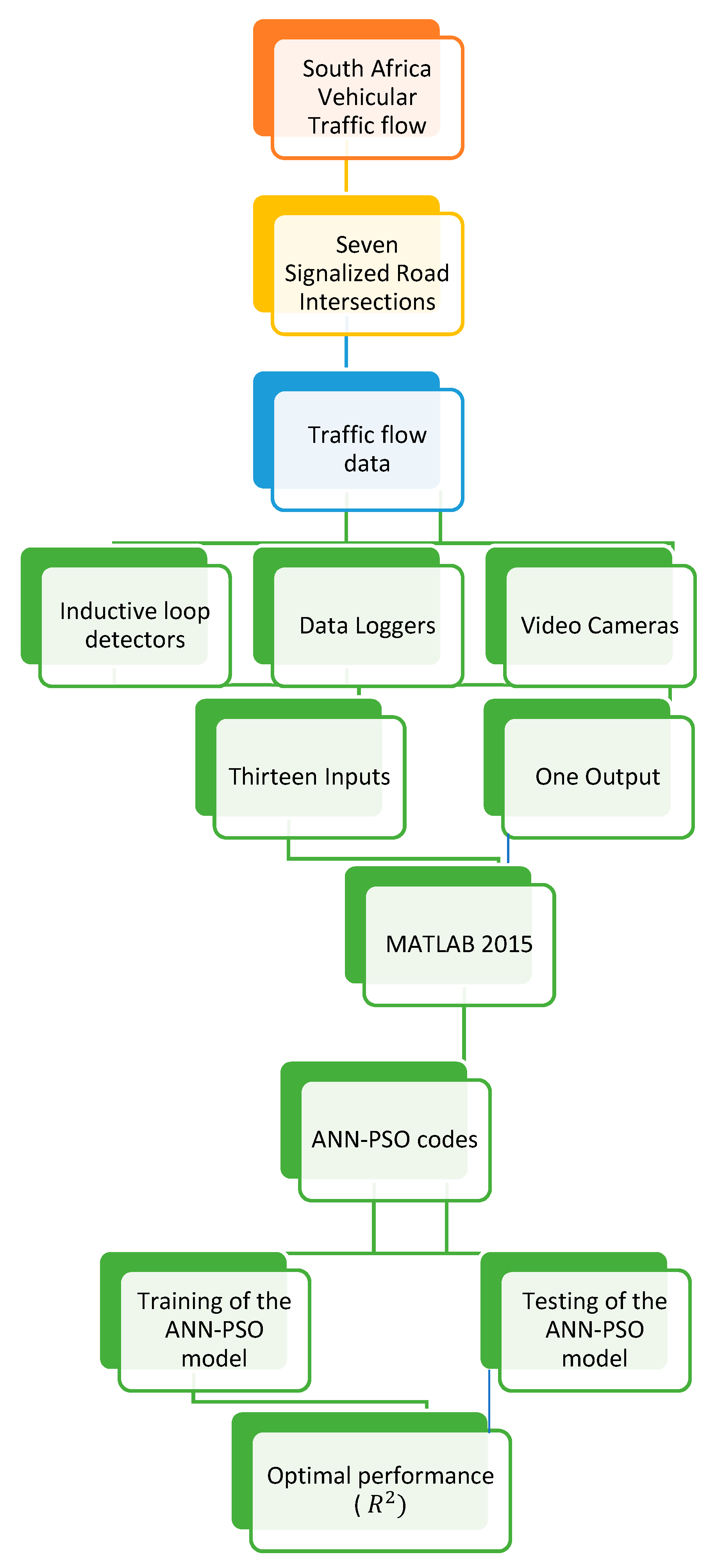
3.1. Research Design

This research study is designed to demonstrate how an artificial neural network trained by particle swarm optimization can model vehicles’ traffic flow at signalized road intersections using selected traffic flow inputs and output. Seven selected signalized road intersections were selected due to their large traffic volume of vehicles on the selected metropolitan section of Gauteng province in South Africa. Figure 1 shows the flowchart of the research methodology applied in this research.

3.2. Traffic Data

The size of the dataset considered in this study is four hundred and thirty-four, and fourteen traffic flow parameters were considered as both inputs and output within the investigation period.

3.3. Data Collection

The method adopted for the collection of data includes the Primary and secondary methods. The primary method used in this research involves collecting traffic data from seven South African signalized road intersections through inductive loop detectors and video cameras. The secondary data was obtained through visitations to the South African Ministry of Transportation and South Africa National Roads Agency Limited (SANRAL) and interaction with Traffic engineers and urban planners’ staff of Mikros traffic Monitoring systems Ltd. (MTM) to obtain relevant information on transportation systems within South Africa.

3.4. Sample and Sampling Techniques

Sampling has to do with choosing a subcategory of individuals from a statistical population to assess the entire population quickly. In the case of this research, the traffic dataset obtained from Mikros Traffic Monitoring Limited was unlimited. A fraction of four hundred and thirty-four and fourteen traffic data was chosen to easily assess the entire population of the South Africa Transportation Network, and we focused on seven roadsites connected to the N1 Allandale freeway in Gauteng Province due to their higher traffic density and traffic volume. The inputs and outputs variables used in this research are the speed of the vehicles, number of different classifications of vehicles, traffic volume, traffic density, the distance covered by the vehicles, and the time it takes the vehicles to travel the road’s length.

3.5. Population of the Study

One of the top-rated companies known for traffic monitoring solutions, specializing in collecting traffic data electronically, constitutes the study population. The company is called Mikros Traffic Monitoring (MTM) Company, a Syntell group subsidiary. This company works in conjunction with the South Africa Ministry of Transportation. Traffic data obtained from MTM for this research study is concentrated on vehicles navigating Gauteng province, South Africa.

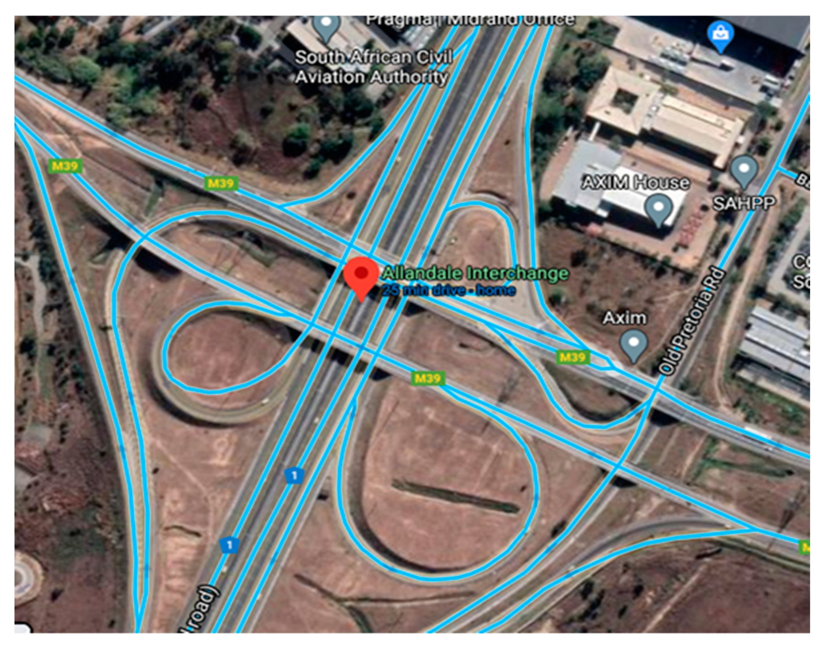
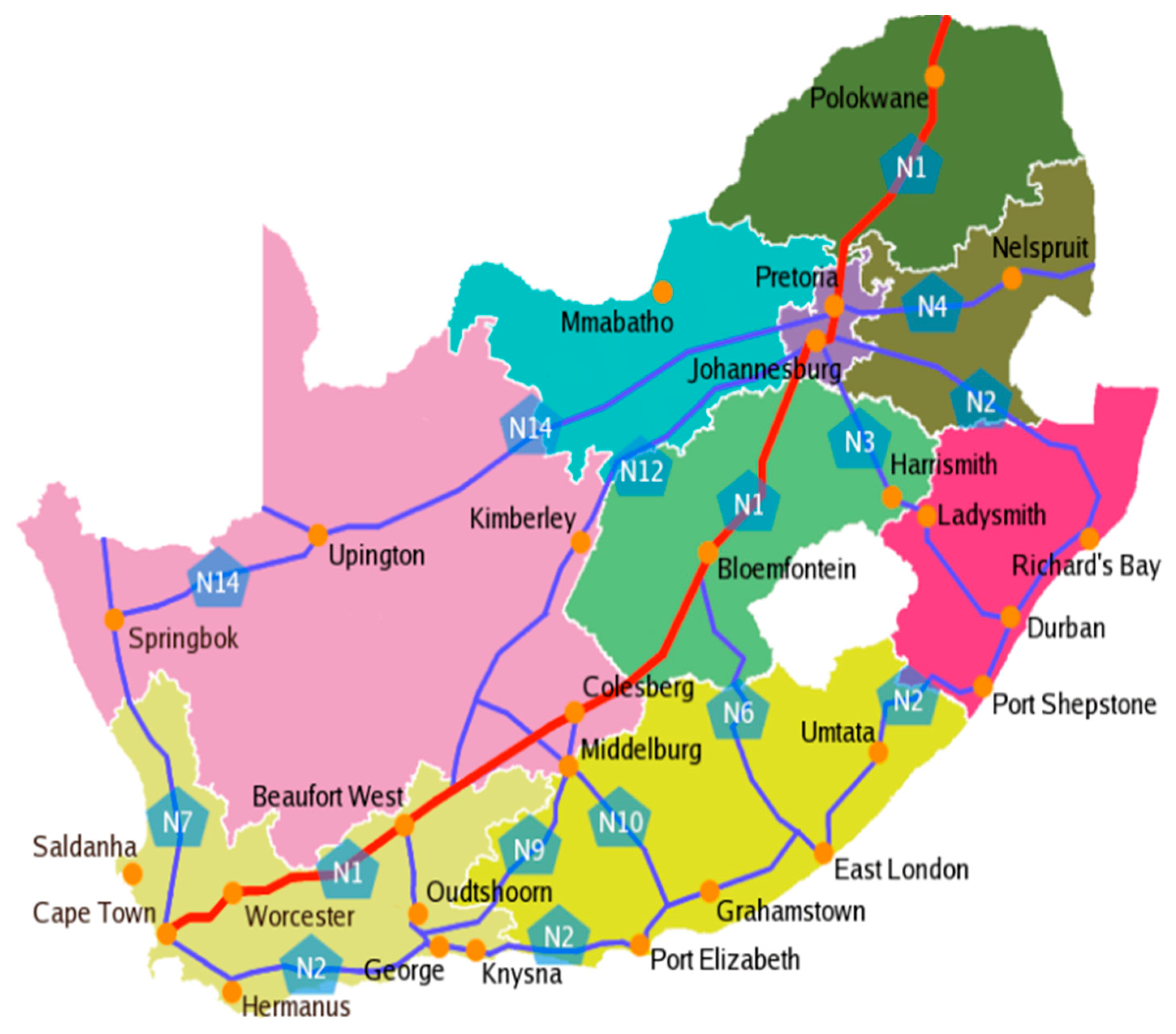
3.6. Location of the Research Study

The Allandale interchange (N1 Ben Schoeman) is one of the busiest and best-rated interchanges in South Africa regarding infrastructure and connectivity. It also connects Johannesburg and Pretoria with an average travel distance of 14.7 km. The aerial drone image of this interchange is shown in Figure 2. This interchange accommodates more than 80,000 vehicles traveling southbound and over 71,000 vehicles moving Northbound every 24-h. Figure 3 shows the N1 Allandale interchange’s description, a South Africa Government (National) road network that connects Johannesburg through Pretoria, Bloemfontein, Polokwane, Capetown, and Beit Bridge (which is located on the border of South Africa and Zimbabwe).

The traffic dataset was obtained from the N1 Ben Schoemann, also known as the Allandale interchange, using inductive loop detectors and roadside video cameras. This interchange is connected to seven different road networks with different lanes and directions. The characteristics of these roadsites are shown in the Appendix A (

Table A1. Features of the Seven Roadsites.

Name of the Roadsites	Dates	Number of Lanes	Lane Descriptions	Directions	Number of Vehicles at Each Roadsites	Longitude	Latitude	Speed Limit (km/hr)	Length of the Roadsites (m)
Brakfontein 1C N1 SB	15–27 July 2019	7	01 Fastlane to Johannesburg	Southbound	2,097,152	28.16857° E	−25.88084° S	120	12.5
			02 Middle to Johannesburg	Southbound
			03 Slow Lane to Johannesburg	Southbound
			04 On-Ramp joining N3	Southbound
			05 Fastlane from N1	Southbound
			06 Middle Lane from N1 (Polokwane)	Southbound
			07 Slow Lane from N1 (Polokwane)	Southbound
Old Johannesburg Road SB Off-Ramp	15–29 July 2019	5	01 Fastlane to Johannesburg	Southbound	16,240,260	28.158402° E	25.90833° S	120	9.4
			02 Middle to Johannesburg	Southbound
			03 Middle to Johannesburg	Southbound
			04 Slow Lane to Johannesburg	Southbound
			05 The Off-Ramp to R10 1N	Southbound
Samrand Avenue Southbound Off-Ramp	15–29 July 2019	7	01 Fastlane to Johannesburg	Southbound	18,448,023	28.146509° E	−25.9271° S	120	7
			02 Middle to Johannesburg	Southbound
			03 Middle to Johannesburg	Southbound
			04 Slow Lane to Johannesburg	Southbound
			05 Off-Ramp to Ultra city	Southbound
			06 Fastlane, Off- Ramp	Southbound
			07 Slow Lane, the Off-Ramp to Samrand Avenue	Southbound
Olifantsfnt SB Off-Ramp	15–29 July 2019	5	01 Fastlane to Johannesburg	Southbound	19,051,124	28.134396° E	−25.95482° S	120	3.7
			02 Middle to Johannesburg	Southbound
			03 Middle to Johannesburg	Southbound
			04 Slow Lane to Johannesburg	Southbound
			05 Off-Ramp to R56 2	Southbound
New Road Southbound (Off-Ramp)	15–29 July 2019	5	01 Fastlane to Johannesburg	Southbound	18,262,048	28.128098° E	25.97556° S	120	1.3
			02 Middle to Johannesburg	Southbound
			03 Middle to Johannesburg	Southbound
			04 Slow Lane to Johannesburg	Southbound
			05 Off-Ramp to New Road	Southbound
Allandale Road Southbound IC (Southbound Only)	15–29 July 2019	3	01 CD Road	Southbound	5,815,648	28.116522° E	−26.01489° S	120	54.5
			02 Off-Ramp to Allandale Road	Southbound
			03 On-Ramp from Allandale Road to N1 South	Southbound
Allandale Road Southbound On-Ramp	15–29 July 2019	8	01 Fastlane to Johannesburg	Southbound	24,292,818	28.11375° E	−26.02054° S	120	53.7
			02 Middle to Johannesburg	Southbound
			03 Middle to Johannesburg	Southbound
			04 Middle to Johannesburg	Southbound
			05 Fastlane to Johannesburg	Southbound
			06 The On-Ramp from Allandale Road Eastbound	Southbound
			07 Fastlane On-Ramp from Southbound Allandale Road Westbound/ South	Southbound
			08 Allandale Road Westbound South	Southbound

); these road networks are:

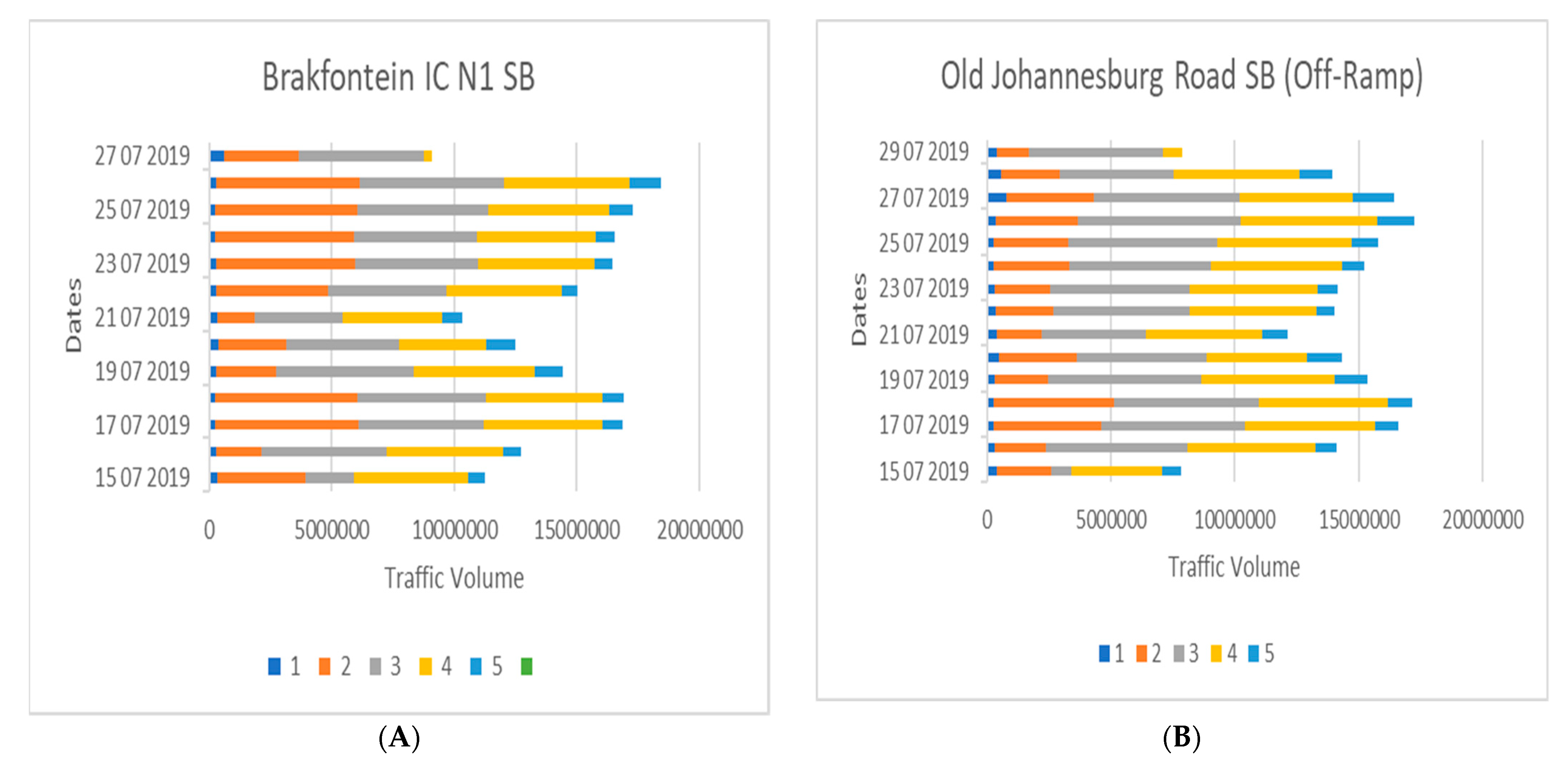
• Brakfontein 1C N1 SB (Roadsite 1852).
• Old Johannesburg Road SB off-ramp (Roadsite 1854).
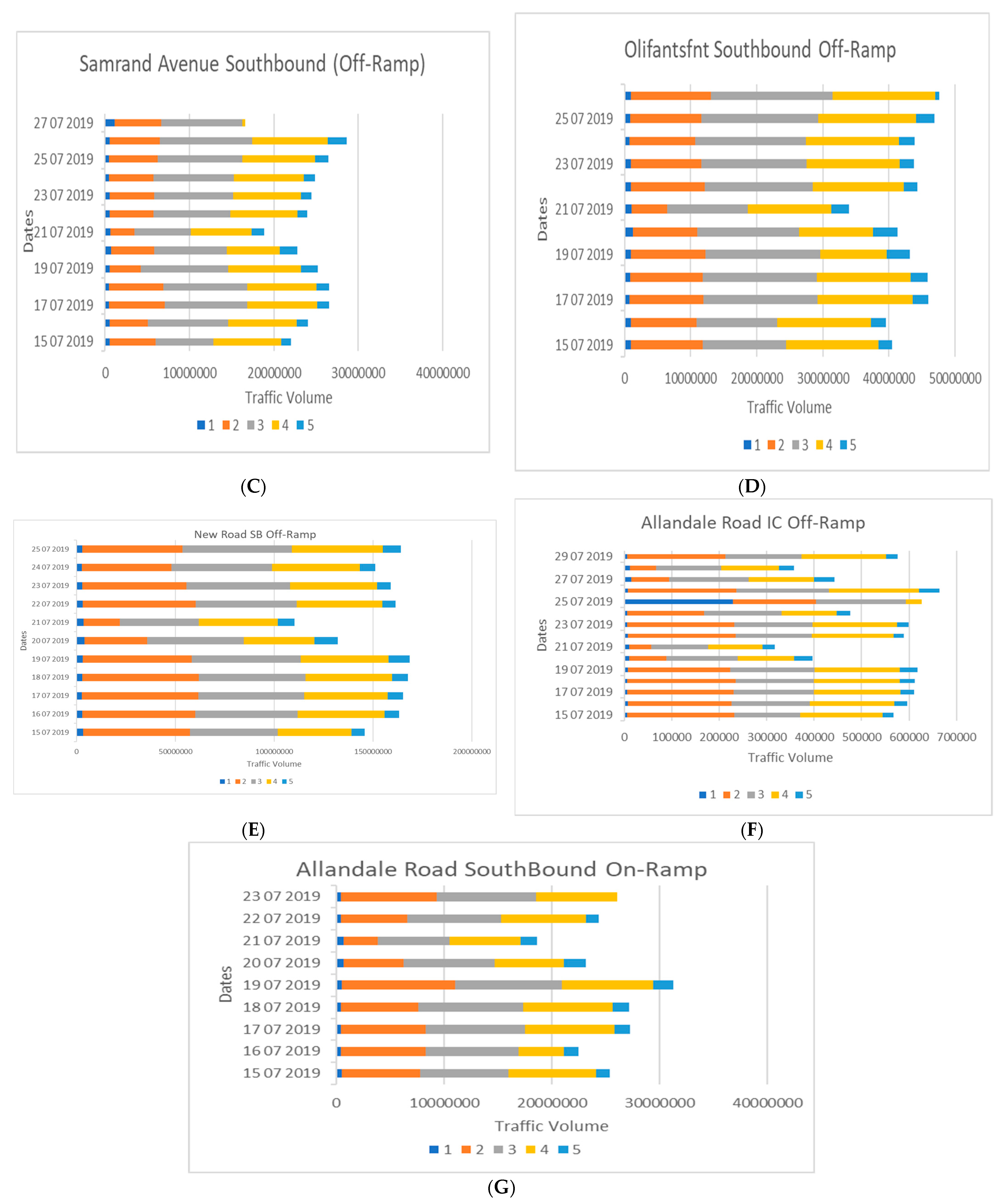
• Samrand Avenue SB off-ramp (Roadsite 1856).
• Olifantsfnt SB off-ramp (Roadsite 1858).
• New road SB off-ramp (Roadsite 1860).
• Allandale road SB IC off-ramp (Roadsite 1862).
• Allandale road SB on-ramp (Roadsite 1863).

Note:

• Off-ramp: When a vehicle drives off the freeway to connect with another road, usually a minor road.
• On-ramp: This is when vehicles connect from the minor road to the freeway

The characteristics of these seven roadsites have been described in detail in Table A1 in Appendix A. The table comprises of the longitude and latitude of each of the roadsites, the number of lanes on each road, number of vehicles on each road, lengths of the road, speed limit, and the direction of the vehicular traffic flow on each roadsites.

3.7. Size and Extraction of the Traffic Datasets

Four hundred and thirty-four traffic datasets were collected under different heterogeneous conditions. From seven road sites on the South Africa Road network, all these road sites are connected to the N1 route, the busiest on the South Africa Road network. The traffic datasets were collected from these seven sites with the aid of various traffic collection equipment. Fourteen different traffic flow parameters were identified from these traffic datasets. These traffic parameters are crucial in understanding the traffic flow patterns of the South Africa Road network. Five traffic flow periods were identified based on the period from the traffic datasets. The five traffic flow periods are identified based on the traffic volume experienced on these roads depending on the day’s specific time. These periods are either off-peak or on-peak, depending on the time during the day. The periods are classified as 1, 2, 3, 4, 5 in this research; this is explained further in Section 3.9. Fourteen of these parameters were used as inputs and output during the artificial neural network-particle swarm optimization modelling. The traffic flow parameters identified in these seven road sites are shown in

Table 2. Categorization of the traffic datasets into inputs and output.

Input Variables	Output Variables
Traffic density	Traffic Volume
Number of light vehicles
The average speed of light vehicles
Time of day of light vehicles
The average speed of a long truck
Time of day of long truck
Number of long trucks
The average speed of a medium truck
Time of day of medium truck
Number of medium trucks
Number of short trucks
The average speed of a short truck
Time of day of short truck

:

• Traffic density: This is the number of vehicles per unit length. It is calculated as:

$$\mathrm{Traffic} \mathrm{density}=\frac{\mathrm{Number} \mathrm{of} \mathrm{vehicles}}{\mathrm{length}}$$

(1)

• Traffic volume: This is the number of vehicles depending on a specific period.

$$\mathrm{Traffic} \mathrm{volume}=\frac{\mathrm{Number} \mathrm{of} \mathrm{vehicles} }{\mathrm{time}}$$

(2)

• The number of short/medium/long trucks: This is the overall total number of different types of trucks on a specific road depending on the time of the day and traffic volume.
• The number of light vehicles: This is the overall total number of different types of light vehicles on a specific road network considering the period of the day and traffic volume.
• Time of day of light vehicles or short/medium/long trucks: This parameter is dependent on the speed of the vehicles or truck and the distance of the specific road site. For example, the road sites used as a case study in this research study have their distance. Its mathematical expression is;

$$\mathrm{speed}=\frac{\mathrm{distance}}{\mathrm{time}} \mathrm{therefore}, \mathrm{time}=\frac{\mathrm{distance}}{\mathrm{speed}}$$

(3)

• The average speed of light vehicles or short/medium/long trucks: This is the speed of the vehicles on the road at a specific period. Each road has its speed limit. The road sites used for this study all have a speed limit of 120 km/h.

The South African Ministry of transportation classified different vehicles into Class 1, Class 2, Class 3, or Class 4. Light vehicles are usually classified as Class 1. In contrast, trucks are classified between Class 2 to Class 4 depending on each truck’s number of axles. In this research, the following are grouped under a light vehicle or short/medium/long truck: 2 axles, 6 tyre unit + light trailer (max 4 axle); three-axle single units (+1 axle trailer); four or fewer axle large trailer(s); five-axle single trailer; fight motor vehicle; light motor vehicle towing; motorcycle; seven axle vehicles; six-axle multi-trailer; six-axle single trailers; two-axle buses; two axles six tyre single unit. The definition of different classifications of vehicles has been provided in the Appendix A section.

3.8. Method of Data Collection

Table 3. Collection of Traffic data.

Traffic Data Collection Equipment	Traffic Data
Data Loggers	Vehicular Speed
Loop Detectors	Vehicular Speed. Distance. Time.
Video Cameras	Number of Vehicles

shows the traffic flow parameters collected by each traffic flow equipment’s. The equipment used for the data collection by Mikros Traffic Monitoring (MTM), a subsidiary of Syntell Group Limited, are:

3.8.1. Data Loggers

Electronic equipment is used in road transportation networks to record data or information garnered for some time by vehicles’ movement on highways and road intersections. An example of a data logger is shown in Figure 4. This information gathered can be analyzed or documented for future purposes. They make use of sensors to record information from vehicles.

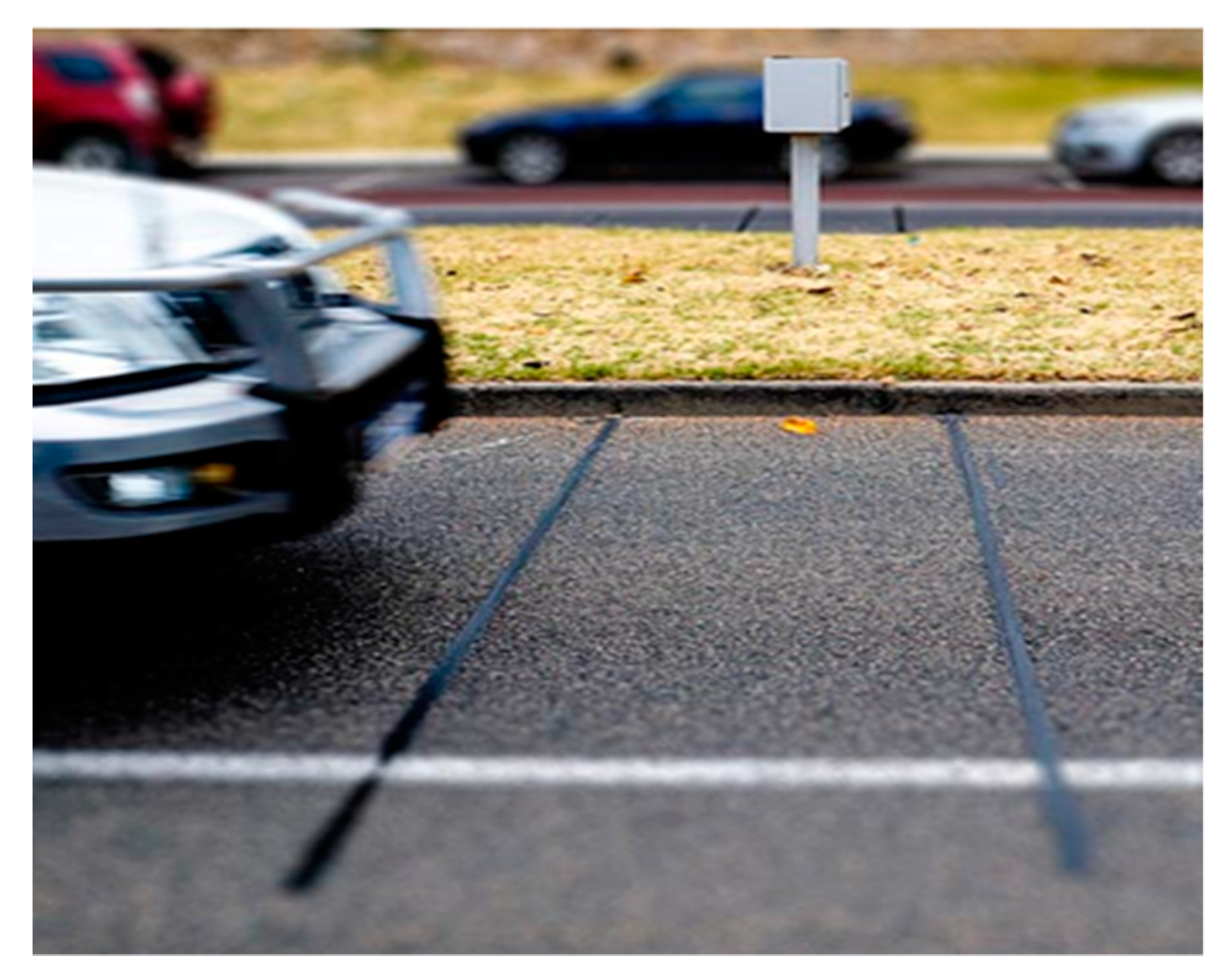
3.8.2. Loop Detectors

They are also called inductive loop detectors (shown in Figure 5). These detectors are installed along with highway bumps or where there is a zebra crossing. Besides, they are always relatively closed to traffic lights. They detect the number of vehicles passing, the speed and distance covered by the vehicles, and the time it took the vehicle to arrive at that position on the road.

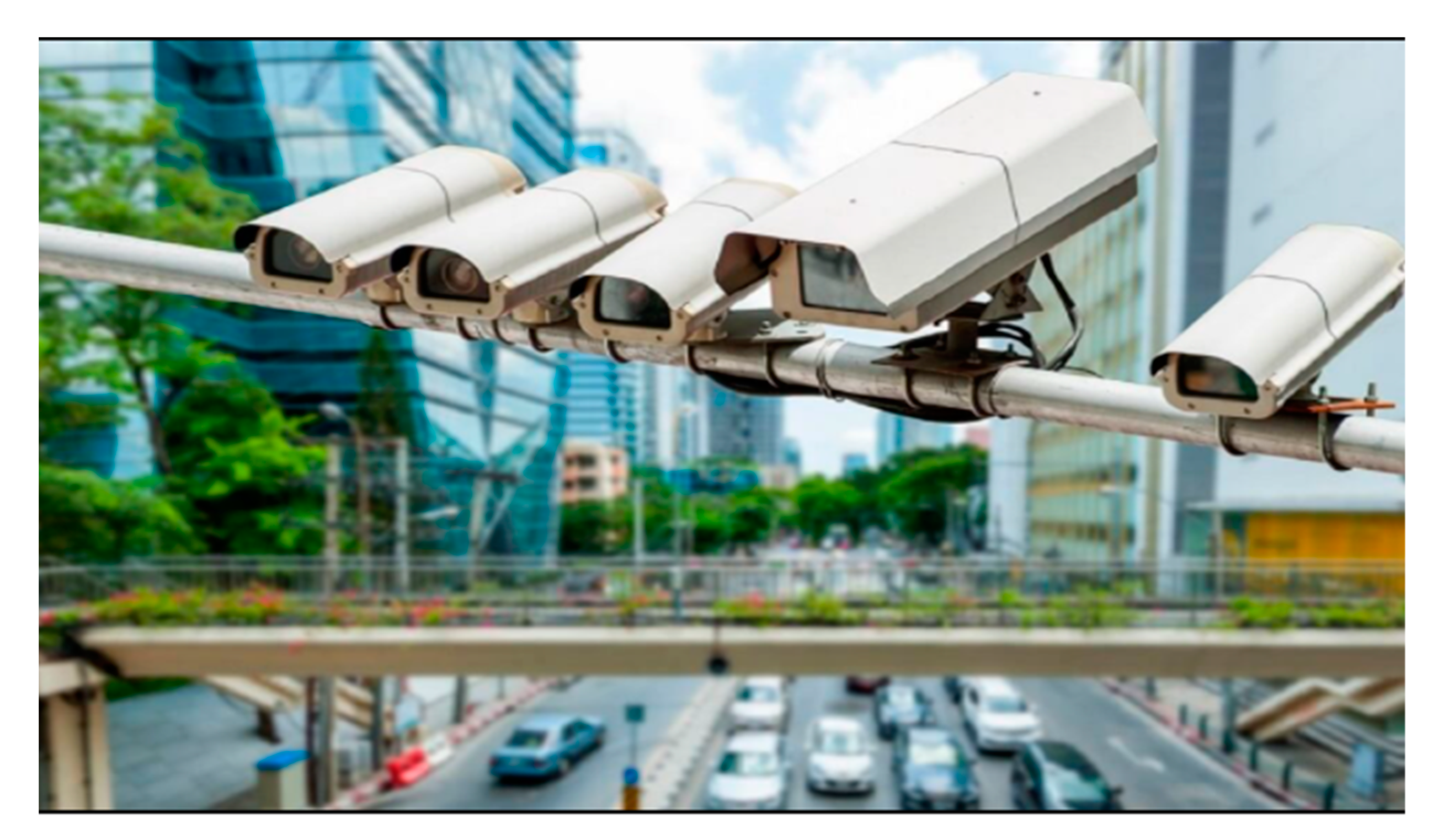
3.8.3. Video Cameras

These are installed on traffic light poles and usually found around road intersections, road tunnels, highways, freeways, and sometimes roundabouts. A typical illustration of this is shown in Figure 6. They are commonly used to catch traffic offenders or monitor the traffic flow of vehicles. The major limitation is that they are always affected by weather conditions, especially during the rainy or harmattan period; during this period, it is difficult for the video cameras to monitor vehicles’ traffic flow on the road.

3.9. South Africa Vehicular Traffic Flow

Note that for this research study, the period of the day is divided as:

1:

00:00:00–04:59:59 (Off-peak)

2:

05:00:00–09:59:59 (On-peak)

3:

10:00:00–14:59:59 (On-peak)

4:

15:00:00–19:59:59 (On-peak)

5:

20:00:00–23:59:59 (Off-peak)

For clarity and understanding of the vehicular traffic volume of each roadsites, the dates and days the traffic datasets were collected are from 15 July 2019 (Monday) to 25 July 2019 (Thursday). Figure A1 (these figures can be found in the Appendix A section, they are numbered A–G) shows the traffic volume of vehicles at each roadsites considering the period of the day. The traffic volume tables for each roadsites can be found in the Appendix A section. They are named Table A1, Table A2,

Table A3. Brakfontein IC N1 SB.

Dates
Period of the Day	15 July 2019	16 July 2019	17 July 2019	18 July 2019	19 July 2019	20 July 2019	21 July 2019	22 July 2019	23 July 2019	24 July 2019	25 July 2019	26 July 2019	27 July 2019
1	321,821	284,516	235,749	255,599	292,933	396,825	346,475	285,355	287,843	234,682	252,186	299,738	610,946
2	3,602,048	1,869,268	5,836,870	5,800,263	2,423,271	2,759,542	1,505,778	4,583,483	5,691,507	5,680,098	5,780,232	5,853,269	3,041,894
3	1,999,604	5,102,335	5,149,346	5,224,989	5,611,289	4,596,207	3,612,345	4,819,565	4,988,628	5,027,838	5,339,309	5,891,051	5,123,845
4	4,646,792	4,734,556	4,827,747	4,775,710	4,951,608	3,534,356	4,022,901	4,675,268	4,746,483	4,834,704	4,952,798	5,114,025	296,582
5	674,526	732,688	824,652	853,587	1,125,768	1,205,557	839,470	653,840	732,518	776,017	938,792	1,285,480

,

Table A4. Old Johannesburg Road Southbound (Off-Ramp).

Dates
Period of the Day	15 July 2019	16 July 2019	17 July 2019	18 July 2019	19 July 2019	20 July 2019	21 July 2019	22 July 2019	23 July 2019	24 July 2019	25 July 2019	26 July 2019	27 July 2019	28 July 2019	29 July 2019
1	390,179	327,976	268,065	289,300	335,488	469,798	417,142	339,721	335,219	270,048	290,175	350,518	773,861	568,289	404,581
2	2,216,559	2,042,699	4,333,069	4,838,127	2,131,202	3,149,843	1,769,578	2,347,645	2,203,855	3,040,326	2,973,499	3,331,478	3,539,626	2,348,912	1,275,185
3	815,676	5,730,636	5,829,798	5,849,334	6,162,667	5,226,996	4,225,467	5,487,717	5,633,324	5,718,815	6,029,431	6,567,132	5,901,943	4,609,278	5,423,568
4	3,644,100	5,144,936	5,203,609	5,203,848	5,399,589	4,057,684	4,701,158	5,094,101	5,137,524	5,279,266	5,407,199	5,485,859	4,527,064	5,071,441	765,203
5	787,586	875,753	960,764	991,788	1,326,893	1,424,255	1,035,343	766,568	837,739	892,657	1,095,860	1,517,427	1,695,464	1,333,457

,

Table A5. Samrand Avenue Southbound (Off Ramp).

Dates
Period of the Day	15 July 2019	16 July 2019	17 July 2019	18 July 2019	19 July 2019	20 July 2019	21 July 2019	22 July 2019	23 July 2019	24 July 2019	25 July 2019	26 July 2019	27 July 2019
1	574,868	504,994	425,123	468,260	531,622	710,172	623,026	520,392	522,734	434,026	477,027	549,520	1,099,849
2	5,416,190	4,544,699	6,666,994	6,469,966	3,682,757	5,135,566	2,821,822	5,240,023	5,280,114	5,273,322	5,765,438	5,956,048	5,588,665
3	6,882,973	9,543,915	9,737,896	9,880,675	10,412,641	8,544,563	6,737,959	9,095,988	9,350,828	9,518,832	10,046,177	10,928,995	9,559,681
4	7,996,735	8,120,977	8,284,089	8,244,838	8,571,413	6,335,493	7,167,665	7,948,635	8,063,400	8,284,807	8,576,608	8,947,607	366,385
5	1,163,614	1,323,411	1,431,353	1,481,270	1,993,989	2,103,922	1,490,162	1,145,786	1,259,688	1,339,216	1,640,843	2,286,731

,

Table A6. Olifantsfnt SB Off-Ramp.

Dates
Period of the Day	15 July 2019	16 July 2019	17 July 2019	18 July 2019	19 July 2019	20 July 2019	21 July 2019	22 July 2019	23 July 2019	24 July 2019	25 July 2019	26 July 2019
1	1,021,527	945,044	797,486	833,213	961,670	1,255,697	1,106,365	968,462	962,808	817,024	883,234	997,146
2	10,823,115	9,909,632	11,188,930	11,043,824	11,309,548	9,732,065	5,347,205	11,174,255	10,663,524	9,850,399	10,791,670	12,106,587
3	12,567,075	12,259,622	17,256,690	17,241,171	17,338,897	15,446,793	12,179,020	16,316,704	15,960,378	16,765,428	17,689,342	18,360,307
4	14,038,494	14,120,725	14,320,182	14,195,183	10,090,051	11,135,014	12,679,847	13,810,047	14,025,189	14,115,094	14,698,109	15,520,252
5	2,045,141	2,287,602	2,457,236	2,557,637	3,472,005	3,738,633	2,645,941	2,023,783	2,193,621	2,314,826	2,820,308	607,144

and

Table A7. Allandale Road IC Off Ramp.

Dates
Period of the Day	15 July 2019	16 July 2019	17 July 2019	18 July 2019	19 July 2019	20 July 2019	21 July 2019	22 July 2019	23 July 2019	24 July 2019	25 July 2019	26 July 2019	27 July 2019	28 July 2019	29 July 2019
1	6,983	7,617	6,508	6,883	8,209	11,286	10,399	7,839	6,941	6,185	228,716	7,956	14,480	11,976	6,939
2	224,281	218,494	224,619	227,947	215,095	77,622	46,099	227,613	225,165	162,713	175,226	227,637	80,516	54,909	205,804
3	138,796	165,058	167,919	165,493	178,113	150,937	120,560	160,484	164,332	162,785	189,282	196,424	167,500	137,369	161,353
4	174,386	177,442	183,483	179,768	179,424	117,872	114,460	171,007	177,787	115,017	33,283	189,045	137,601	122,157	176,988
5	23,199	27,515	28,339	31,839	36,712	38,355	25,727	22,364	25,031	29,796		42,752	42,704	30,649	25,172

. The traffic flow system depends on the traffic volume at a certain period of the day. For example, in each of the roadsites, the period between (00:00:00–04:59:59) is when the traffic flow is gradually building up. This is a period between midnight and the early morning when people are just starting to their place of work. Between 05:00:00–09:59:59 and 10:00:00–14:59:59 is the on-peak period, this when the traffic volume attains the maximum number of vehicles on the road. This is usually when traffic congestion occurs due to high road traffic density (large vehicle occupancy on the road). The traffic congestion can be either recurrent (this occurs when the route is heavily used because of its network connectivity) and non-recurrent (this might be due to road accidents or unforeseeable circumstances on the road). The exception among these vehicular traffic flows is that during the non-working days, which are Saturday and Sunday, from critical observation, between the period of 00:00:00–04:59:59 and 05:00:00–09:59:59, there is a low traffic volume due to people not going to place of work at this period of the day. During these days (Saturday and Sunday), the traffic flow only started to build up in the afternoon, around 15:00:00 and 19:59:59. When the traffic flow is high, the traffic density will increase, which means that the traffic volume will be high, i.e., high traffic volume means there are many vehicles on the road. The traffic flow periods have shed light on one thing, to understand traffic flow, it is crucial that we first have clarity on the traffic volume, traffic density, and the period of the day (off-peak and on-peak).

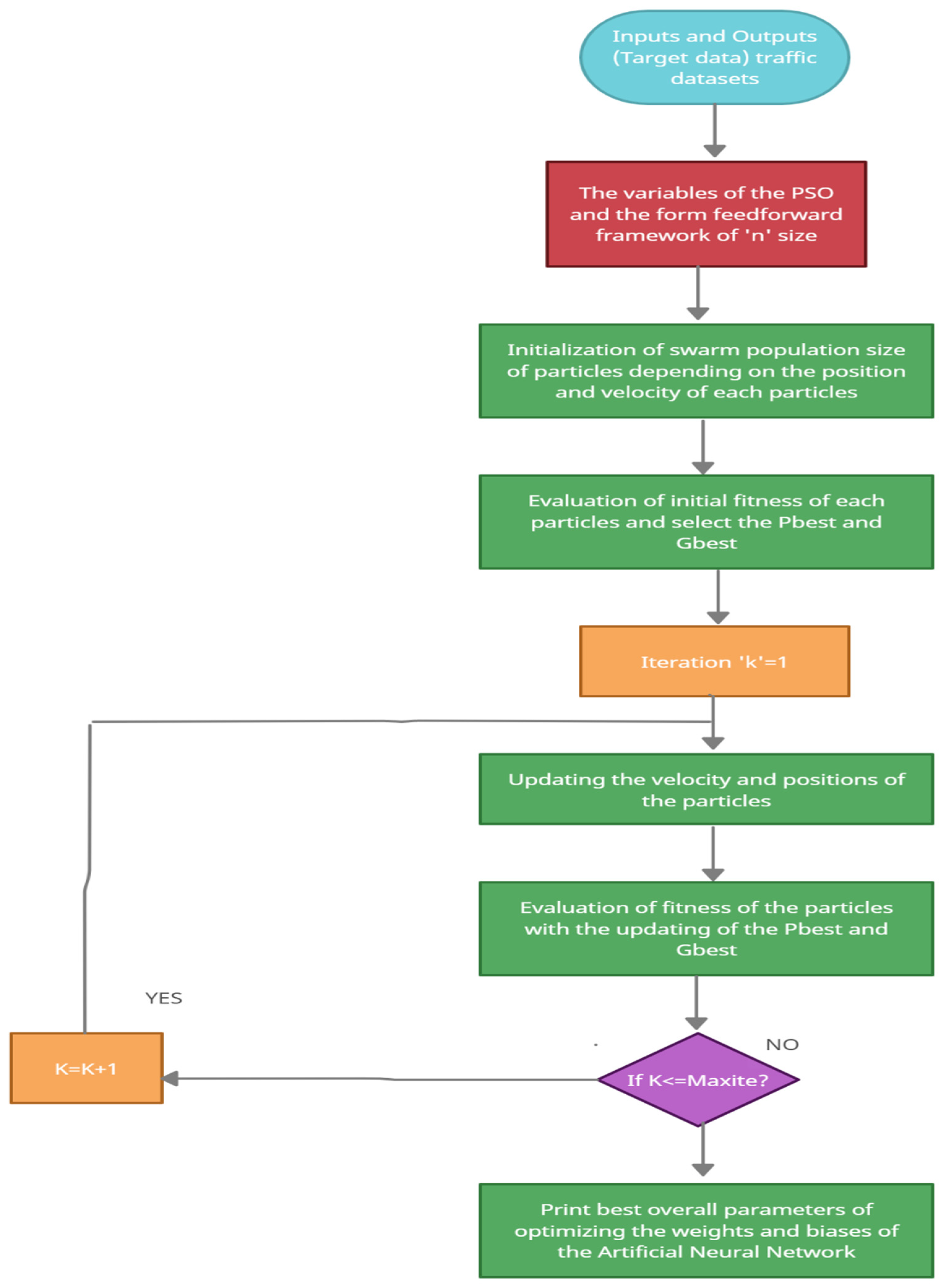
3.10. The Goal, Data Inputs, and Data Processing Involved in the Development of the ANN-PSO Model

Particle swarm optimization is a strong and effective metaheuristic algorithm that resolves complicated and non-linear optimization problems [58]. This swarm optimization technique can efficiently solve global optimization issues compared with other classical optimization techniques. Particle swarm optimization is a modern optimization technique dependent on social methods such as fish schooling and bird flocking [59]. Depending on the mathematical conceptual framework of particle swarm optimization, these three significant parameters play important roles in PSO optimizations: position, velocity, and fitness. The primary steps of PSO to solve any complex optimization issues is as follows:

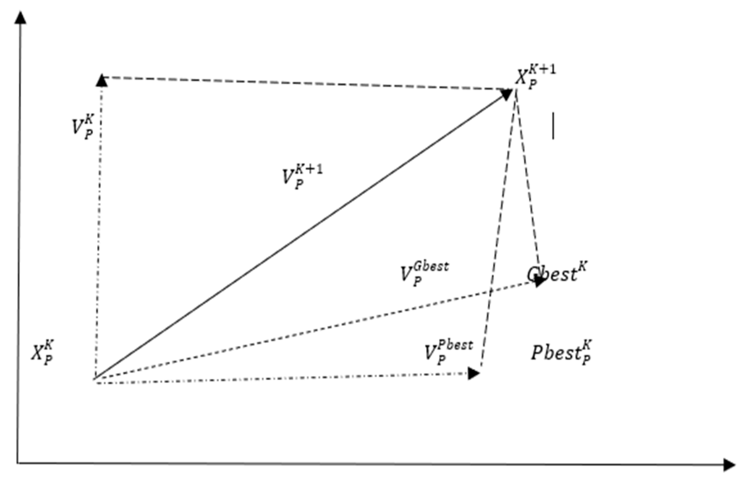
• Initializing a population of individuals (particles) with random velocities and positions in the domain of the problem.
• Computing the fitness value for all particles.
• Investigating fitness of particles.
• Updating the velocity and position of particles using Equations (4) and (5).

$$V_{ij}^t=\chi \left[\omega {\upsilon }_{ij}^{t-1}+c_1{r}_1\left(p_{ij}^{t-1}-x_{ij}^{t-1}\right)+c_2{r}_2\left(G_j^{t-1}-x_{ij}^{t-1}\right)\right]$$

(4)

$$x_{ij}^t=x_{ij}^{t-1}+{\upsilon }_{ij}^t$$

(5)

• r₁ and r₂ are called random numbers.
• c₁ and c₂ are the acceleration constants.
• w, χ, P^t and G^t are all called the weight of inertia, pbest, and gbest.

When an artificial neural network is adequately trained in the MATLAB environment, it will function as a black-box model, explaining the relationship between a complex dataset, which comprises an input and output (irrespective of the number of variables). An artificial neural network consists of mathematical processing units called neurons. These neurons can be found in the black box during a neural network operation on MATLAB. These neurons can form a relationship with each other via weights and biases. An artificial neural network consists of three primary layers: the input, hidden, and output layers. The neurons are placed in the hidden and output layers, while the input layers do not contain any neurons. After the neural network toolbox has been opened in MATLAB, training will be conducted with the input data and the corresponding output datasets.

The inputs in Table 2 were divided into 13 columns; the output datasets are in a single column on another excel sheet. These are all carried out to determine the appropriate weights and biases of the neurons. Neural network training of data (input and outputs) means determining the optimum variables of different weights and biases of the neural network. Generally, different methods are applied to determine the appropriate parameters of weights and biases of the Artificial Neural Network. In this research, the suitable optimum training of the network has been done by applying an artificial intelligence technique called Artificial Neural Network—Particle Swarm Optimization, which can be found in the MATLAB software environment.

Once the ANN-PSO training has been done adequately on the datasets, the network validation is performed using the testing data-independent variables. An artificial neural network is perfect if the fitness function values are lower or closer to one for the training and validation of the traffic datasets. Particle swarm optimization is created through different species’ social and cooperative behaviour to fill the loopholes in a multidimensional search space. The PSO algorithm is based on the personal experience ($Pbest$), the overall personal experience of the species ($Gbest$), and the decision m particles’ decision-making to determine the subsequent positions in the search space. Furthermore, the personal experience of different types of species are accelerated by two (2) main factors called $C_1$ and $C_2$ and a pair of (no specific variables random) $r_1$ and $r_2$ which are created between a variable ranging from 0 to 1, while the movement is multiplied by ‘w’, which is a crucial inertia factor ‘w’.

$$V_{p,q}^{K+1}=w\times V_{p,q}^K+c_1{r}_1\left(Pbes{t}_{p,q}^k-X_{p,q}^K\right)+c_2{r}_2\left(Gbes{t}_q^k-X_{p,q}^K\right)$$

(6)

$$X_{p,q}^{K+1}=X_{p,q}^K+V_{p,q}^{K+1}$$

(7)

In Equation (6), $Pbes{t}_{p,q}^k$ denotes the personal best of the $q\mathrm{th}$ component of the $p\mathrm{th}$ individual, while the $Gbes{t}_q^k$ referred to $q\mathrm{th}$ component of the best individual species of the population of iteration ‘k’. Figure 7 shows the search mode of operation of a particle swarm optimization. The initial $Pbest$ of each particle is the position, and the initial $Pbest$ is the most appropriate particle position between a randomly initialized population. The $Pbest$ and $Gbest$ of each particle are:

$$\begin{gathered} If f\left(X_P^{K+1}\right)<f\left(Pbes{t}_P^K\right) then Pbes{t}_P^{K+1} \\ =X_P^{K+1} else Pbes{t}_P^{K+1}=Pbes{t}_P^K \end{gathered}$$

(8)

$$\begin{gathered} \mathrm{If} f\left(X_P^{K+1}\right)<f\left(Gbes{t}^K\right) \mathrm{then} Gbes{t}^{K+1} \\ =X_P^{K+1} else Gbes{t}^{K+1}=Gbes{t}^K \end{gathered}$$

(9)

The flowchart below shows the steps been applied to train the artificial neural network using particle swarm optimization. In the early stages, ‘N’ sets of weights and biases of the size of particles ‘D’, directly proportional to ‘n*(m + 2) + 1’ applied randomly. Each traffic dataset is a particle in particle swarm optimization, which is depicted as the particle position. Presently, the initial velocity of each particle in the traffic dataset is applied as 10% of the current position of the correlated particle (which is referred to as ‘V’). The fitness ‘f’ of each particle in the traffic dataset undergoes evaluation. The corresponding particles to the optimum performance of the fitness named as Gbest while Pbest of each particle are accepted as their corresponding bearings. Equations (6) and (9) are used to upgrade the positions of each particle in the PSO, resulting in conclusive optimized weights and biases of the ANN traffic model. A typical flowchart shows an ANN-PSO-based model in Figure 8.

A programming language has been inbuilt in the MATLAB environment, assuming that there is a three-layer artificial neural network architecture. The number of input and output variables considered for developing the artificial neural network-particle swarm optimization model is shown in Table 2. In this study, the number of neurons used varies between five (5) and ten (10), respectively. The ANN-PSO model has variables, which are dependent on particle swarm optimization or the artificial neural network. The PSO variables include the overall number of particles in the swarm population size (swarm size, N), acceleration factor associated with the particle velocity ($C_1$ and $C_2$), the inertial weight of the particles (w). The artificial neural network features are the network architecture (i.e., the total number of neurons in the hidden layer ‘n’). The inertia weight of the particles is commonly known as random numbers, which are primarily within the range of 0–1.

A comprehensive iteration was carried out on the ANN-PSO model for obtaining an appropriate combination of variables related to the traffic data. Six different numbers of neurons were considered; the variables are 5, 6, 7, 8, 9, and 10. Six (6) distinct swarm population sizes were also considered. According to past research work [60], it was discovered that the best possible optimum value of the acceleration factor of the particle $C_1$ and $C_2$ is situated in-between 1–2.5 and 2–3. Five (5) various variables of accelerating factors $C_1$ and $C_2$ were considered.

Table 4. Values of parameters of the ANN-PSO model used for the traffic study.

	Acceleration Factor		Swarm Population Size	Number of Neurons
Value of the parameters	C1	C2
	1	2.0	10	5
	1.5	2.25	20	6
	2	2.5	50	7
	2.25	2.75	100	8
	2.5	3.0	200	9
			400	10

shows the overall number of neurons in the hidden layer used to train the datasets. The table also presents the particle size and the acceleration factor considered when training the traffic datasets. The variables of the PSO-ANN hybrid model developed for the traffic data were established by performing frequent training of the traffic data. An overall 1000 training runs were done on the MATLAB environment to acquire the near-perfect integration of the ANN-PSO framework. Training of the traffic data during the ANN-PSO training of the traffic data. The training will only be stopped or terminated when the objective function iteration has been fulfilled. The following benchmark was adhered to. The benchmark is:

• A maximum iteration of 1000.
• The training run will be terminated if the objective function is not up to a specific fixed parameter.

The ANN-PSO training was carried out in the MATLAB environment by following these steps:

• Step One: Traffic data collection.
• Step Two: Creation of the hybrid network.
• Step Three: Configuration of the ANN-PSO network.
• Step Four: Initialization of the weight and biases.
• Step Five: Training the Neural network by applying particle swarm optimization.
• Step Six: Validation and testing of the ANN-PSO network.
• Step Seven: Using the Neural Network.

The inputs and outputs variables used for the development of the ANN-PSO network are shown in Table 2. These input and output variables were categorized based on the method used by [61,62]. Preparation of the dataset is followed by structuring the architecture of the algorithms. MATLAB user interface tools and command-line functionality are used to oversee the ANN-PSO model’s development, training, and testing. The traffic datasets used in this traffic prediction study were obtained from seven major road intersections connecting to the N1 Allandale Road, the busiest interchange in southern Africa. The breakdown of how the traffic datasets were divided and used for the ANN-PSO training and testing is shown in

Table 5. The Breakdown of the Roadsites traffic datasets for ANN-PSO training.

Roadsites	Training	Testing	Total
Brakfontein 1C N1 SB (Roadsite 1852)	51	10	61
Old Johannesburg road SB off-ramp (Roadsite 1854)	64	10	74
Samrand Avenue SB off-ramp (Roadsite 1856)	54	10	64
Olifantsfnt SB off-ramp (Roadsite 1858)	50	10	60
New road SB off-ramp (Roadsite 1860)	47	10	57
Allandale road SB IC off-ramp (Roadsite 1862)	64	10	74
Allandale road SB on-ramp (Roadsite 1863)	34	10	44
	364	70	434

below. We used 434 traffic datasets, 364 for training, and 70 for testing the ANN-PSO model performance. The division of the traffic datasets for training and testing is shown in Table 5 below. The MATLAB codes used to develop the ANN-PSO model have been deposited in a GitHub repository. This is the link to the MATLAB codes https://github.com/Olayode1989/ANN-PSO-codes.git (accessed on 20 August 2021).

Allendale road SB on, Allendale Road IC (SB only), new road SB off, Olifantsfnt road SB off, Samrand Ave SB off, Old Johannesburg Road SB off and Brakfontein IC N1 SB. Equations (10) and (11) show the regression value’s statistical formulae and the mean square error.

$$R^2=1-\frac{{\sum }_k{\left(y_k-{\widehat{y}}_k\right)}^2}{{\sum }_k{\left(y_k-{\overline{y}}_k\right)}^2}$$

(10)

$$MSE=\frac{1}{2} {\displaystyle \sum }_{k=1}^n{\left(y_k-{\widehat{y}}_k\right)}^2$$

(11)

where $y_k$, ${\widehat{y}}_k$, ${\overline{y}}_k$ n represents the experimental data sample, the values predicted by the algorithm, the mean value of the experimental data samples, and the number of data samples, respectively. The primary code file used for training the traffic datasets using ANN-PSO was generated. These codes were saved as ‘m_pso_m’ before the ANN-PSO was used to prepare the traffic data. The input and output datasets were created and saved in a Microsoft Excel worksheet. In the Microsoft worksheet, two sheets were created, namely sheet 1 and sheet 2. In sheet 1, it consists of the input datasets and sheet two, which comprises the output (traffic volume) and the target data required to be placed in the first column of the first row of sheet 2 in the excel file. This Microsoft excel of the input and output data (target data) must be saved with the name ‘datafile.xlsx’ and kept in the same directory as the ANN-PSO codes. These traffic data can be uploaded into the MATLAB environment by inputting the following command codes in the MATLAB command window:

• [x,t] = traffic_dataset;
• Inputs =X′;
• Outputs = t′;

All three files were saved in the MATLAB directory ‘myfunc.m’, ‘nn_pso.m’, and datafile. xslx to train the artificial neural network using Particle swarm optimization effectively. The ‘nn_pso.m’ file is run consistently depending on the number of hidden neurons, swarm population size, and accelerating factor. For example, if the number of hidden neurons is five (5) and the swarm population size is 10, the best performing accelerating factor is $C_1$ = 2.25 and $C_2$ = 2. These parameters will be changed in the ‘nn_pso.m’ codes inside the MATLAB environment.

4. Results and Discussions

The ANN-PSO Model Results and Discussions

The 434 traffic datasets obtained from the seven roadsites were divided into 367 and 70 for training and testing. To achieve the best optimum output, the trial-and-error approach was used to discover the best value for the number of hidden nodes, iterations, and acceleration factors. Sigmoid and linear functions were used for the ANN-PSO model for the hidden and output node activation functions. The best optimal parameters for both training and testing performance of the ANN-PSO model of traffic flow at each roadsites, as shown in

Table 6. The Parametric analysis of ANN-PSO Hybrid Model for the Traffic Dataset.

Number of Neurons	Swarm Population Size	C1	C2	Training (R2)	MSE	Testing (R2)
5	10	2.25	2	0.97306	47.128	0.9314
5	20	2.25	2	0.96982	52.781	0.7838
5	50	1.5	2.25	0.98313	29.734	0.9769
5	100	1	2.75	0.97102	50.590	0.9784
5	200	1.5	2	0.98566	25.228	0.8660
5	400	1.5	2	0.98356	28.921	0.9822
6	10	1	3	0.98452	27.227	0.9423
6	20	2	2.25	0.97620	41.817	0.9781
6	50	1	2.5	0.98758	22.007	0.8595
6	100	1	2.5	0.99172	14.694	0.8917
6	200	1	2.75	0.96347	63.516	0.9681
6	400	1	2.25	0.98569	25.173	0.9140
7	10	1.5	2.5	0.98005	35.093	0.8268
7	20	1	2.75	0.98942	18.736	0.9353
7	50	1	2.5	0.98819	20.849	0.9411
7	100	1	2.5	0.99299	12.453	0.9591
7	200	1.5	2.25	0.99314	12.199	0.9486
7	400	2	2	0.98688	23.118	0.9661
8	10	1	2.75	0.97769	39.122	0.9546
8	20	1	2.5	0.98570	25.162	0.9401
8	50	1.5	2.25	0.99391	10.849	0.9276
8	100	1	2.5	0.98571	25.128	0.9100
8	200	1	2.75	0.98816	20.877	0.9716
8	400	1	2.25	0.99490	90.219	0.8880
9	10	1	2.75	0.98235	31.076	0.9356
9	20	1	3	0.96028	69.016	0.9800
9	50	1.5	2.25	0.99290	12.598	0.9090
9	100	2	2	0.98634	24.048	0.7637
9	200	1.5	2.25	0.98993	17.757	0.8790
9	400	1	2.5	0.99361	11.290	0.8218
10	10	1	2.75	0.97468	44.281	0.9897
10	20	1.5	2.5	0.97177	49.340	0.9564
10	50	1.5	2.5	0.97826	38.098	0.8602
10	100	1	2.75	0.99122	15.536	0.9627
10	200	1	2.75	0.99078	16.265	0.9056
10	400	1.5	2.5	0.98950	18.500	0.9246

, are:

(a)

Number of hidden neurons = 5

(b)

Swarm population size = 400

(c)

Number of traffic datasets = 434

(d)

C₁ and C₂ = 1.5 and 2

(e)

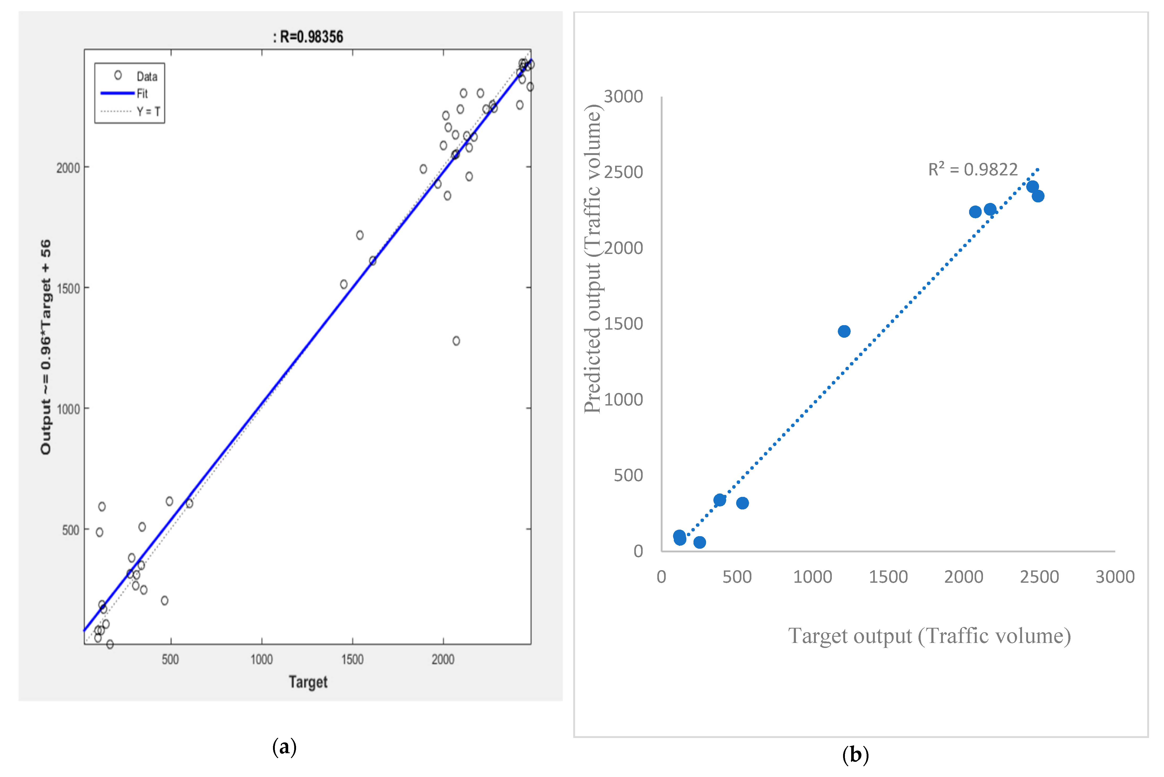
Training (R²) = 0.98356

(f)

Testing (R²) = 0.98220

Figure 9a below shows the result of the ANN-PSO training response of 0.98356, considering the number of hidden neurons, accelerating factors, and swarm population sizes. To evaluate the accuracy of the ANN-PSO model, observed and predicted output of the traffic volume of vehicles at each roadsites were compared in Figure 9b, with the testing performance of the model been 0.98220. The ANN-PSO model’s testing performance of the traffic datasets from the roadsites was calculated by plotting a graph between the actual value of the traffic volume and the simulated traffic volume achieved during the ANN-PSO model training testing and validation. The existing traffic volume was compared with the simulated traffic volume to determine the ANN-PSO model’s validity of each roadsites traffic dataset.

The study set out to determine if an artificial network trained by particle swarm optimization can be used to model traffic flow at a signalized road intersection. The current study has been able to answer that question, considering Table 6, which shows evidently that the ANN-PSO model is capable of modelling traffic flow at a signalized road intersection. The most interesting finding from the ANN-PSO results shows that the best optimum training and testing performed for the roadsites was obtained with a different number of neurons, swarm population sizes, and acceleration factors $C_1$ and $C_2$. From the results, it can be concluded that the ANN-PSO’s parameters affect the performance prediction of the traffic flow datasets. Another significant finding from the ANN-PSO result is that the accelerating factors and mean square error plays an essential role in determining the optimum performance of each ANN-PSO model on each roadsites; for example, the lower the MSE, the more likely there is going to be an optimum training or testing performance of the ANN-PSO model. The most striking result to emerge from the research study is that when an ANN-PSO model comprises the maximum correlation coefficient ($R^2$) and the minimum MSE, it can be said that the ANN-PSO model is superior. The training and testing performance regression value for the roadsites indicates that the inputs and target are well correlated. Another significant finding is that when R-value is closer to 1, this means that there is an accurate linear relevance between the traffic inputs and target.

5. Conclusions and Future Work

To achieve the aim of this research study, an in-depth and exhaustive research study has been conducted to develop an ANN-PSO capable of modelling and analysing vehicular traffic flow at a signalized road intersection. For the accurate modelling of traffic flow, it was important to understand and identify some traffic flow parameters and have clarity on how traffic flow affects the movement of vehicles at a signalized road intersection. In this research study, the successful development of the ANN-PSO model for the traffic flow of vehicles at a signalized road intersection has been achieved. The vehicular speed, the time of the day, the traffic volume, and the traffic density of each class of vehicles (light vehicles, long trucks, medium trucks, and short trucks) have been considered as the traffic flow inputs and outputs variables. The following conclusions can be drawn from this present study:

• ANN-PSO model is potentially suitable for the prediction and analysis of traffic flow at a signalized road intersection. This model could be used to predict traffic flow with a high level of accuracy. It explains the heterogeneous traffic flow conditions at different periods of the day.
• Due to the stochastic nature of traffic information, it is difficult to determine the volume of traffic flow at a signalized road intersection. This equally implies that the specific time of the day determines the traffic density and vehicular speed on the road. The evidence from this study suggests that traffic density and traffic volume are significant in determining traffic congestion and understanding the traffic flow patterns on a road transportation network.
• The ANN-PSO model developed in this study will assist transportation engineers and urban planners in developing possible ways to use their respective country’s traffic information to understudy traffic flow patterns and variables for effective predictive models. Also, designing a traffic control system for traffic lights at road intersections can be made possible and timely.
• The results of this study will serve as a base for future studies for engineers and transportation researchers in understanding the complexity of traffic flow patterns at a signalized road intersection. Also, it will assist drivers in the decision-making process, such as which period of the day traffic congestion is likely to occur on a particular road.

Based on the results obtained from this research study, this research study has thrown up many questions in need of further investigation in the field of transportation:

• Further work needs to be done to establish whether other metaheuristic algorithms, such as the second generation of particle swarm optimization (SGPSO), bee colony, an artificial neural network trained by genetic algorithm (ANN-GA), adaptive neuro-fuzzy inference system trained by particle swarm optimization (ANFIS-PSO) and simulated annealing can be used in developing predictive models using traffic flow parameters obtained from a signalized road intersection.
• A natural progression of this research study would be to focus on unsignalized road intersections, traffic light timing response optimization, and the usability of traffic volume in determining traffic congestions at road intersections. Besides, demonstrating other metaheuristic techniques’ strength and predictive power will be very useful as a comparative measure for minimizing traffic issues in road transportation.
• Finally, another possible area of future research would be to investigate if the optimal solution obtained in this research depends on factors affecting traffic flow and how could the optimal solution change depending on these factors.

References

1. Li, Z.; Schonfeld, P. Hybrid simulated annealing and genetic algorithm for optimizing arterial signal timings under oversaturated traffic conditions. J. Adv. Transp. 2015, 49, 153–170. [Google Scholar] [CrossRef]
2. Xu, H.; Zhuo, Z.; Chen, J.; Fang, X. Traffic signal coordination control along oversaturated two-way arterials. PeerJ Comput. Sci. 2020, 6, e319. [Google Scholar] [CrossRef]
3. Khan, M.U.; Saeed, S.; Nehdi, M.L.; Rehan, R. Macroscopic Traffic-Flow Modelling Based on Gap-Filling Behavior of Heterogeneous Traffic. Appl. Sci. 2021, 11, 4278. [Google Scholar] [CrossRef]
4. Ranjan, N.; Bhandari, S.; Khan, P.; Hong, Y.-S.; Kim, H. Large-Scale Road Network Congestion Pattern Analysis and Prediction Using Deep Convolutional Autoencoder. Sustainability 2021, 13, 5108. [Google Scholar] [CrossRef]
5. Drop, N.; Garlińska, D. Evaluation of Intelligent Transport Systems Used in Urban Agglomerations and Intercity Roads by Professional Truck Drivers. Sustainability 2021, 13, 2935. [Google Scholar] [CrossRef]
6. Olayode, I.; Tartibu, L.; Okwu, M.; Uchechi, U. Intelligent transportation systems, un-signalized road intersections and traffic congestion in Johannesburg: A systematic review. Procedia CIRP 2020, 91, 844–850. [Google Scholar] [CrossRef]
7. Van Brummelen, J.; O’Brien, M.; Gruyer, D.; Najjaran, H. Autonomous vehicle perception: The technology of today and tomorrow. Transp. Res. Part. C Emerg. Technol. 2018, 89, 384–406. [Google Scholar] [CrossRef]
8. Kuutti, S.; Fallah, S.; Katsaros, K.; Dianati, M.; Mccullough, F.; Mouzakitis, A. A survey of the state-of-the-art localization techniques and their potentials for autonomous vehicle applications. IEEE Internet Things J. 2018, 5, 829–846. [Google Scholar] [CrossRef]
9. Garner, D.; Louw, J.; Burnett, S. Towards resolving congestion in Gauteng. In Proceedings of the SATC—South African Transport Conference Meeting the Transport Challenges in Southern Africa, Johannesburg, South Africa, 16–20 July 2001. [Google Scholar]
10. Olayode, O.; Tartibu, L.; Okwu, M. Application of Artificial Intelligence in Traffic Control System of Non-autonomous Vehicles at Signalized Road Intersection. Procedia CIRP 2020, 91, 194–200. [Google Scholar] [CrossRef]
11. Chakwizira, J. The question of road traffic congestion and decongestion in the greater Johannesburg area: Some perspectives. In Proceedings of the SATC—South African Transport Conference Meeting the Transport Challenges in Southern Africa, Johannesburg, South Africa, 9–12 July 2007. [Google Scholar]
12. AlRashidi, M.R.; El-Hawary, M.E. A survey of particle swarm optimization applications in electric power systems. IEEE Trans. Evol. Comput. 2008, 13, 913–918. [Google Scholar] [CrossRef]
13. Jain, N.K.; Nangia, U.; Jain, A. PSO for multiobjective economic load dispatch (MELD) for minimizing generation cost and transmission losses. J. Inst. Eng. Ser. B 2016, 97, 185–191. [Google Scholar] [CrossRef]
14. Abido, M.A. Optimal power flow using particle swarm optimization. Int. J. Electr. Power Energy Syst. 2002, 24, 563–571. [Google Scholar] [CrossRef]
15. Liang, R.-H.; Tsai, S.-R.; Chen, Y.-T.; Tseng, W.-T. Optimal power flow by a fuzzy based hybrid particle swarm optimization approach. Electr. Power Syst. Res. 2011, 81, 1466–1474. [Google Scholar] [CrossRef]
16. Salomon, C.P.; Lambert-Torres, G.; Martins, H.G.; Ferreira, C.; Costa, C.I. Load flow computation via particle swarm optimization. In Proceedings of the 2010 9th IEEE/IAS International Conference on Industry Applications-INDUSCON, Sao Paulo, Brazil, 8–10 November 2010; pp. 1–6. [Google Scholar]
17. Acharjee, P.; Goswami, S. Chaotic Particle Swarm Optimization based reliable algorithm to overcome the limitations of conventional power flow methods. In Proceedings of the 2009 IEEE/PES Power Systems Conference and Exposition, Washington, DC, USA, 15–18 March 2009; pp. 1–7. [Google Scholar]
18. Gaing, Z.-L. A particle swarm optimization approach for optimum design of PID controller in AVR system. IEEE Trans. Energy Convers. 2004, 19, 384–391. [Google Scholar] [CrossRef] [Green Version]
19. Yapıcı, H.; Çetinkaya, N. An improved particle swarm optimization algorithm using eagle strategy for power loss minimization. Math. Probl. Eng. 2017, 2017, 1063045. [Google Scholar] [CrossRef] [Green Version]
20. Nimtawat, A.; Nanakorn, P. Simple particle swarm optimization for solving beam-slab layout design problems. Procedia Eng. 2011, 14, 1392–1398. [Google Scholar] [CrossRef]
21. Mac, T.T.; Copot, C.; Tran, D.T.; de Keyser, R. A hierarchical global path planning approach for mobile robots based on multi-objective particle swarm optimization. Appl. Soft Comput. 2017, 59, 68–76. [Google Scholar] [CrossRef]
22. Islam, M.J.; Li, X.; Mei, Y. A time-varying transfer function for balancing the exploration and exploitation ability of a binary PSO. Appl. Soft Comput. 2017, 59, 182–196. [Google Scholar] [CrossRef]
23. Suresh, A.; Harish, K.; Radhika, N. Particle swarm optimization over back propagation neural network for length of stay prediction. Procedia Comput. Sci. 2015, 46, 268–275. [Google Scholar] [CrossRef] [Green Version]
24. Zou, R.; Kalivarapu, V.; Winer, E.; Oliver, J.; Bhattacharya, S. Particle swarm optimization-based source seeking. IEEE Trans. Autom. Sci. Eng. 2015, 12, 865–875. [Google Scholar] [CrossRef] [Green Version]
25. Wen, P.; Zhi, M.; Zhang, G.; Li, S. Fault prediction of elevator door system based on PSO-BP neural network. Engineering 2016, 8, 761–766. [Google Scholar] [CrossRef] [Green Version]
26. Gong, T.; Tuson, A.L. Particle swarm optimization for quadratic assignment problems-a forma analysis approach. Int. J. Comput. Intell. Res. 2008, 4, 177–185. [Google Scholar] [CrossRef]
27. Liu, Z.; Zhao, R. Equipment Possession Quantity Modeling and Particle Swarm Optimization. In Proceedings of the 2009 Third International Conference on Genetic and Evolutionary Computing, Guilin, China, 14–17 October 2009; pp. 628–632. [Google Scholar]
28. Li, J.-q.; Pan, Q.-k.; Xie, S.-x.; Jia, B.-x.; Wang, Y.-t. A hybrid particle swarm optimization and tabu search algorithm for flexible job-shop scheduling problem. Int. J. Comput. Theory Eng. 2010, 2, 189. [Google Scholar] [CrossRef] [Green Version]
29. Bhushan, B.; Pillai, S.S. Particle swarm optimization and firefly algorithm: Performance analysis. In Proceedings of the 2013 3rd IEEE International Advance Computing Conference (IACC), Ghaziabad, UP, India, 22–23 February 2013; pp. 746–751. [Google Scholar]
30. Angeline, P.J. Using selection to improve particle swarm optimization. In Proceedings of the 1998 IEEE International Conference on Evolutionary Computation Proceedings, IEEE World Congress on Computational Intelligence (Cat. No. 98TH8360), Anchorage, AK, USA, 4–9 May 1998; pp. 84–89. [Google Scholar]
31. Chen, Y.-P.; Peng, W.-C.; Jian, M.-C. Particle swarm optimization with recombination and dynamic linkage discovery. IEEE Trans. Syst. ManCybern. Part B 2007, 37, 1460–1470. [Google Scholar] [CrossRef]
32. Sharaf, A.M.; El-Gammal, A.A. A novel discrete multi-objective Particle Swarm Optimization (MOPSO) of optimal shunt power filter. In Proceedings of the 2009 IEEE/PES Power Systems Conference and Exposition, Seattle, WA, USA, 15–18 March 2009; pp. 1–7. [Google Scholar]
33. Goh, C.K.; Tan, K.C.; Liu, D.; Chiam, S.C. A competitive and cooperative co-evolutionary approach to multi-objective particle swarm optimization algorithm design. Eur. J. Oper. Res. 2010, 202, 42–54. [Google Scholar] [CrossRef]
34. Harrison, K.R.; Ombuki-Berman, B.; Engelbrecht, A.P. Knowledge Transfer Strategies for Vector Evaluated Particle Swarm Optimization; Technical Report CS-12-07; Brock University, Department of Computer Science: St. Catharines, ON, Canada, 2012. [Google Scholar]
35. Benedetti, M.; Azaro, R.; Massa, A. Memory enhanced PSO-based optimization approach for smart antennas control in complex interference scenarios. IEEE Trans. Antennas Propag. 2008, 56, 1939–1947. [Google Scholar] [CrossRef]
36. Duan, H.; Li, P.; Yu, Y. A predator-prey particle swarm optimization approach to multiple UCAV air combat modeled by dynamic game theory. IEEE/CAA J. Autom. Sin. 2015, 2, 11–18. [Google Scholar]
37. Liang, J.J.; Qin, A.K.; Suganthan, P.N.; Baskar, S. Comprehensive learning particle swarm optimizer for global optimization of multimodal functions. IEEE Trans. Evol. Comput. 2006, 10, 281–295. [Google Scholar] [CrossRef]
38. Li, C.; Yang, S.; Nguyen, T.T. A self-learning particle swarm optimizer for global optimization problems. IEEE Trans. Syst. ManCybern. Part. B Cybern. 2011, 42, 627–646. [Google Scholar]
39. Zhan, Z.-H.; Zhang, J.; Li, Y.; Shi, Y.-H. Orthogonal learning particle swarm optimization. IEEE Trans. Evol. Comput. 2010, 15, 832–847. [Google Scholar] [CrossRef] [Green Version]
40. Schutte, J.F.; Groenwold, A.A. A study of global optimization using particle swarms. J. Glob. Optim. 2005, 31, 93–108. [Google Scholar] [CrossRef]
41. Liu, W.-B.; Wang, X.-J. An evolutionary game based particle swarm optimization algorithm. J. Comput. Appl. Math. 2008, 214, 30–35. [Google Scholar] [CrossRef] [Green Version]
42. Hossen, M.S.; Rabbi, F.; Rahman, M.M. Adaptive Particle Swarm Optimization (APSO) for multimodal function optimization. Int. J. Eng. Technol. 2009, 1, 98–103. [Google Scholar]
43. Benmessahel, B.; Touahria, M. An improved combinatorial particle swarm optimization algorithm to database vertical partition. J. Emerg. Trends Comput. Inf. Sci. 2011, 2, 130–135. [Google Scholar]
44. Ji, W.; Wang, K. An improved particle swarm optimization algorithm. In Proceedings of the 2011 International Conference on Computer Science and Network Technology, Harbin, China, 24–26 December 2011; pp. 585–589. [Google Scholar]
45. Safa, M.; Shariati, M.; Ibrahim, Z.; Toghroli, A.; Bin, B.S.; Norazman, M.N.; Petkovic, D. Potential of adaptive neuro fuzzy inference system for evaluating the factors affecting steel-concrete composite beam’s shear strength. Steel Compos. Struct. 2016, 21, 679–688. [Google Scholar] [CrossRef]
46. Mohammadhassani, M.; Nezamabadi-Pour, H.; Suhatril, M.; Shariati, M. An evolutionary fuzzy modelling approach and comparison of different methods for shear strength prediction of high-strength concrete beams without stirrups. Smart Struct. Syst. Int. J. 2014, 14, 785–809. [Google Scholar] [CrossRef]
47. Shariati, M.; Faegh, S.S.; Mehrabi, P.; Bahavarnia, S.; Zandi, Y.; Masoom, D.R.; Toghroli, A.; Trung, N.-T.; Salih, M.N.A. Numerical study on the structural performance of corrugated low yield point steel plate shear walls with circular openings. Steel Compos. Struct. 2019, 33, 569–581. [Google Scholar]
48. Sharafi, P.; Rashidi, M.; Samali, B.; Ronagh, H.; Mortazavi, M. Identification of factors and decision analysis of the level of modularization in building construction. J. Archit. Eng. 2018, 24, 04018010. [Google Scholar] [CrossRef]
49. Taheri, E.; Firouzianhaji, A.; Usefi, N.; Mehrabi, P.; Ronagh, H.; Samali, B. Investigation of a method for strengthening perforated cold-formed steel profiles under compression loads. Appl. Sci. 2019, 9, 5085. [Google Scholar] [CrossRef] [Green Version]
50. Ahmadi, R.; Rashidian, O.; Abbasnia, R.; Nav, F.M.; Usefi, N. Experimental and numerical evaluation of progressive collapse behavior in scaled RC beam-column subassemblage. Shock Vib. 2016, 2016. [Google Scholar] [CrossRef]
51. Nguyen, H.; Drebenstedt, C.; Bui, X.-N.; Bui, D.T. Prediction of blast-induced ground vibration in an open-pit mine by a novel hybrid model based on clustering and artificial neural network. Nat. Resour. Res. 2020, 29, 691–709. [Google Scholar] [CrossRef]
52. Olayode, I.O.; Tartibu, L.K.; Okwu, M.O. Traffic flow Prediction at Signalized Road Intersections: A case of Markov Chain and Artificial Neural Network Model. In Proceedings of the 2021 IEEE 12th International Conference on Mechanical and Intelligent Manufacturing Technologies (ICMIMT), Cape Town, South Africa, 12 July 2021; pp. 287–292. [Google Scholar]
53. Kennedy, J.; Eberhart, R.C. A discrete binary version of the particle swarm algorithm. In Proceedings of the 1997 IEEE International Conference on Systems, Man, and Cybernetics. Computational Cybernetics and Simulation, Orlando, FL, USA, 12–15 October 1997; Volume 5, pp. 4104–4108. [Google Scholar]
54. Atashpaz-Gargari, E.; Lucas, C. Imperialist competitive algorithm: An algorithm for optimization inspired by imperialistic competition. In Proceedings of the 2007 IEEE Congress on Evolutionary Computation, Singapore, 25–28 September 2007; pp. 4661–4667. [Google Scholar]
55. Lazzús, J.A.J.M.; Modelling, C. Neural network-particle swarm modeling to predict thermal properties. Math. Comput. Model. 2013, 57, 2408–2418. [Google Scholar] [CrossRef]
56. Xing, B.; Gao, W.-J. Cat Swarm Optimization Algorithm. In Innovative Computational Intelligence: A Rough Guide to 134 Clever Algorithms; Springer: Berlin, Germany, 2014; pp. 93–104. [Google Scholar]
57. Celtek, S.A.; Durdu, A.; Alı, M.E.M. Real-time traffic signal control with swarm optimization methods. Measurement 2020, 166, 108206. [Google Scholar] [CrossRef]
58. Kennedy, J.; Eberhart, R. Particle swarm optimization. In Proceedings of the ICNN’95-International Conference on Neural Networks, Perth, WA, Australia, 1 December 1995; Volume 4, pp. 1942–1948. [Google Scholar]
59. Eberhart, R.C.; Shi, Y.; Kennedy, J. Swarm Intelligence; Elsevier: Amsterdam, The Netherlands, 2001. [Google Scholar]
60. Alam, M.N.; Das, B.; Pant, V. A comparative study of metaheuristic optimization approaches for directional overcurrent relays coordination. Electr. Power Syst. Res. 2015, 128, 39–52. [Google Scholar] [CrossRef]
61. Kumar, K.; Parida, M.; Katiyar, V. Short term traffic flow prediction for a non urban highway using artificial neural network. Procedia Soc. Behav. Sci. 2013, 104, 755–764. [Google Scholar] [CrossRef] [Green Version]
62. Goves, C.; North, R.; Johnston, R.; Fletcher, G. Short term traffic prediction on the UK motorway network using neural networks. Transp. Res. Procedia 2016, 13, 184–195. [Google Scholar] [CrossRef] [Green Version]
Figure 1. Research methodology.
Applsci 11 08387 g001
Figure 2. An aerial drone image of the Allandale interchange.
Applsci 11 08387 g002
Figure 3. An illustrative description of the N1 (the red line) route through the South Africa Road transportation network.
Applsci 11 08387 g003
Figure 4. A road intersection in Johannesburg showing the data loggers beside the road.
Applsci 11 08387 g004
Figure 5. The black lines on the road surface are the inductive loop detectors.
Applsci 11 08387 g005
Figure 6. Video cameras attached to a traffic signal light.
Applsci 11 08387 g006
Figure 7. The Particle Swarm Optimization search technique for pth particle at a kth objective function in the search field.
Applsci 11 08387 g007
Figure 8. A framework of the ANN-PSO Model developed for the traffic flow prediction performance.
Applsci 11 08387 g008
Figure 9. (a) ANN-PSO training response of the best performance neural network of the traffic datasets of the roadsites (13-5-1). (b) Comparison between the measured and predicted traffic volume of the roadsites for the testing performance of the ANN-PSO model.
Applsci 11 08387 g009