Article

FLRW Cosmological Models with Dynamic Cosmological Term in Modified Gravity

by
Rishi Kumar Tiwari
1,†,
Aroonkumar Beesham
2,*,†,‡ and
Bhupendra Kumar Shukla
3,†
1
Department of Mathematics, Govt Model Science College, Rewa 486003, India
2
Department of Mathematical Sciences, University of Zululand, P Bag X1001, Kwa-Dlangezwa 3886, South Africa
3
Department of Mathematics, Pandit S N Shukla University, Shahdol 484001, India
*
Author to whom correspondence should be addressed.
These authors contributed equally to this work.
Alternate address: Faculty of Natural Sciences, Mangosuthu University of Technology, Jacobs 4026, South Africa.
Universe 2021, 7(9), 319; https://doi.org/10.3390/universe7090319
Submission received: 30 June 2021 / Revised: 26 July 2021 / Accepted: 28 July 2021 / Published: 28 August 2021

Abstract

:
Although the standard lambda cold dark matter cosmological model is quite successful in describing the universe, there are still several issues that are still not resolved. Some of these are the cosmological constant problem, certain anomalies in the cosmic microwave background radiation and whether general relativity is valid on large scales. Therefore, it is interesting to examine modified theories in an attempt to solve these problems, and to examine the entire range of possibilities that are allowed. In this work, we examine one of these modified theories, viz., f(R,T) gravity. We study the homogeneous and isotropic models in this theory, which have some pleasing features, such as no initial singularity, a dynamic cosmological term, and a transition from early deceleration to late-time acceleration as intimated by observations. The physical parameters of the model, as well as the energy conditions, are discussed and a viable cosmological model can be constructed.

1. Introduction

The most widely accepted theory to study the evolution of the universe is, undoubtedly, Einstein’s general theory of relativity, which predicts that the universe was condensed into a very small, hot, and dense state initially, and then expanded. In recent times, observations of type Ia supernova indicate that the current rate of expansion of the universe is accelerating [1,2]. After this, many observations have supported the idea of an accelerated expansion [3,4]. In order to explain this acceleration, a new form of energy has been postulated that has a repulsive effect called dark energy (DE) [5,6,7]. According to the Planck mission team’s best estimate [6], the universe is made up of three forms of matter/energy, viz., 68.5 % dark energy, 26.6 % dark matter, and only 4.9 % baryonic matter.
The most favoured explanation for dark energy is Einstein’s cosmological constant [8,9] which is obtained by adding a cosmological constant to the equations of Einstein’s standard Friedmann–Lemaitre–Robertson–Walker (FLRW) equations, and leads to the lambda cold dark matter or concordance model [6]. This has a solution that includes accelerated expansion and it is widely accepted as the best solution to the dark energy problem [10]. However, the lambda cold dark matter model has several problems associated with it, such as the existence of anomalies in the cosmic microwave background radiation and on small scales, the initial big-bang singularity, the predictability and testability of the inflationary paradigm, the cosmological constant problem, the validity of general relativity on large scales, and the particle nature of dark matter [10]. Basically, the cosmological constant problem is the following [11]: particle physics predicts a constant that is approximately 10 120 times larger than the currently observed value of the constant. This problem has still not been solved, despite much research in the area. One possibility is a dynamic cosmological parameter [12] which can either fit the observations [13], or fit them even better than the standard Λ CDM model [14].
The dark energy associated with the standard Λ C D M model is constant. An important quantity relating to dark energy is the equation of state ω in cosmology, which is the relation between the pressure p and the energy density ρ of the cosmic fluid. Nowadays, a great deal of effort is being expended in observational cosmology to analyze models of dark energy with different equations of state, which are not necessarily constant. Quintessence is a dynamic scalar field with equation of state ω p / ρ > 1 . Another case is the phantom model of dark energy [15,16,17], with equation of state ω < 1 in which there is a future singularity due to the increasing density of dark energy [18,19,20]. Apart from this, several other scalar field models have been proposed such as spintessence [21], k-essence [22,23], quintom [24], the tachyon [25,26], and chameleon [27] with different equation of state parameters. Another category of alternative thought is to come up with a dark fluid, which unites both dark matter and dark energy [28]. Holographic dark energy is one of the contenders which has been suggested in which dark energy originates as a quantum fluctuation of space-time. For detailed reviews on dark energy and its contenders, we refer to these excellent articles [10,29,30,31,32,33,34,35,36].
In another direction, the reason for the acceleration of the universe can be sought in modified gravity theories, for example, f ( R ) , f ( T ) , and f ( G ) , where f ( G ) is modified Gauss–Bonnet gravity, f ( G ) being a general function of the Gauss–Bonnet term. Harko, et al. [37] introduced f ( R , T ) gravity, in which the usual action of general relativity is replaced by a function of T and R, where T is the trace of the energy momentum tensor and R is the Ricci scalar. Furthermore, the T dependence in the action of f ( R , T ) theory could conceivably be due to the existence of some imperfection as there can be some quantum effects, such as intrinsic particle production [38]. This theory allows for an explanation of accelerated expansion without dark energy, and for an avoidance of the initial singularity. Many studies have been conducted in f ( R , T ) gravity, and we list just a few such as perturbations, [39] energy conditions, [40,41,42] thermodynamics, [43,44] wormhole solutions [45,46,47], higher dimensions [48,49] and interacting matter components [50,51]. It is possible to attain a violation of energy conservation [52], and this is something which still needs to be fully investigated. It may be pointed out that the theory is, in some sense, general relativity with a modified matter part, thus allowing for a dynamic cosmological parameter [53]. This allows for the possibility of solving the cosmological constant problem.
In this paper, we reconstruct the FLRW model in f ( R , T ) theory, focusing on a variable cosmological parameter. This correspondence has not been fully studied. We find a model that exhibits a transition from deceleration in the past, to current acceleration. The behaviour of the physical parameters is analysed, as are the energy conditions. The cosmological parameter varies from being large at early times, and decreases to a small value today.
This paper is based on results presented at the “1st International Electronic Conference on Universe” and is a much extended version of the abbreviated paper that appeared in the conference proceedings [54].

2. Basic Equations

In f ( R , T ) gravity, the action is:
S = 1 16 π f ( R , T ) + L m g d x 4 .
where f ( R , T ) is an arbitrary function of the Ricci scalar R, and the trace T of the energy–momentum tensor T i j , i.e., ( T = g i j T i j ), g is the determinant of the metric tensor g i j , and L m is the matter Lagrangian density. The definition of the energy–momentum tensor T μ ν is:
T μ ν = 2 g δ g L m δ g μ ν ,
It is assumed that the Lagrangian density ( L m ) of matter depends not on the derivatives of the components ( g μ ν ) but only on the metric ( g μ ν ) itself. This leads to:
T μ ν = g μ ν L m 2 L m g μ ν .
We note that f ( R , T ) gravity is a generalisation of general relativity, which can also be considered as an extension of the f ( R ) gravity.
Since the field equations in f ( R , T ) gravity also depend on the physical nature of the matter field (through the tensor Θ μ ν as we shall see shortly), each functional form of f leads to a different theoretical model. The three most used forms of f are:
f ( R , T ) = R + 2 f ( T ) ,
f ( R , T ) = f 1 ( R ) + f 2 ( T ) ,
f ( R , T ) = f 1 ( R ) + f 2 ( R ) f 3 ( T ) .
The usual choice for the function f ( R , T ) which we shall use here is [37]:
f ( R , T ) = f 1 ( R ) + f 2 ( T ) ,
i.e., a sum of two independent functions of R and T, respectively.
To obtain the field equations in f ( R , T ) gravity, the action for the field and matter has to varied and then and equated to zero. Varying the action S in Equation (1) with respect to the metric tensor g i j , we obtain the field equations in f ( R , T ) gravity as:
f 1 ( R ) R i j 1 2 ( f 1 ( R ) + f 2 ( T ) ) g i j + ( g i j i j ) f 1 ( R ) = 8 π T i j f 2 ( T ) T i j f 2 ( T ) Θ i j ,
where i j is the D’Alembertian operator, and the prime denotes the derivative with respect to its argument. The tensor Θ i j is defined as
Θ i j = g l m δ T l m δ g i j .
We assume the following forms [55] for the functions f 1 ( R ) and f 2 ( T )
f 1 ( R ) = λ 1 R , f 2 ( T ) = λ 2 T ,
where λ 1 and λ 2 are arbitrary coupling constants of f ( R , T ) gravity. We take the matter content in the universe to be a perfect fluid whose energy momentum tensor is given by:
T i j = ( ρ + p ) u i u j p g i j ,
where p and ρ are the pressure and energy density and of the fluid, respectively, and u i is four velocity vector normalised by u i u i = 1 . From the equation L m = p , Equation (9) becomes:
Θ i j = 2 T i j p g i j ,
Because of this, the field Equation (8) takes the form
f 1 ( R ) R i j 1 2 ( f 1 ( R ) + f 2 ( T ) ) g i j + ( g i j i j ) f 1 ( R ) = 8 π T i j f 2 ( T ) T i j f 2 ( T ) p g i j ,
Using Equations (9)–(12), Equation (13) becomes:
R i j 1 2 R g i j = 8 π + λ 2 λ 1 T i j + λ 2 λ 1 p + 1 2 T g i j .
Note that this equation reduces to the general relativistic limit when we put λ 1 = 1 , λ 2 = 0 .
Now, in the general theory of relativity, the Einstein field equations with cosmological term are:
R i j 1 2 R g i j = T i j + Λ g i j ,
We notice a similarity between Equations (14) and (15). Hence, if we take λ 1 to be approximately unity, and λ 2 to be small, we can set:
Λ Λ ( T ) = λ 2 λ 1 ( p + 1 2 T ) ,
This leads naturally to a varying cosmological parameter Λ as a function of T in f ( R , T ) gravity. Hence, we may also regard f ( R , T ) gravity with the function f given by Equation (10) as equivalent to general relativity, but with a modified matter term, i.e., the addition of a dynamic cosmological parameter. Evaluating the trace T from Equation (11), we obtain:
Λ = λ 2 2 λ 1 ( ρ p ) .
This equation gives the dynamic cosmological parameter in terms of the density ρ and pressure p in f ( R , T ) gravity.
We consider the flat FLRW metric:
d s 2 = d t 2 a 2 ( t ) i = 1 3 d x i 2 ,
where a ( t ) is the scale factor. The Hubble and deceleration parameters are defined by, respectively:
H = a ˙ a ,
q = a ¨ a a ˙ 2 .
with the metric (18), the field Equation (14) become:
3 H 2 = 8 π + λ 2 λ 1 + λ 2 2 λ 1 ρ λ 2 2 λ 1 p ,
2 H ˙ + 3 H 2 = 8 π + λ 2 λ 1 + λ 2 2 λ 1 p + λ 2 2 λ 1 ρ ,
and we achieve the pressure and energy density from the above two equations as
ρ = λ 1 ( 8 π + 2 λ 2 ) 3 + λ 2 ( 8 π + λ 2 ) ( q + 1 ) H 2 ,
p = λ 1 ( 8 π + 2 λ 2 ) 3 + ( 16 π + 3 λ 2 ) ( 8 π + λ 2 ) ( q + 1 ) H 2 ,
and then, the cosmological parameter from Equation (17) as:
Λ = λ 2 ( 8 π + 2 λ 2 ) ( 2 q ) H 2 ,
and the equation of state parameter ( ω = p / ρ ) is given by
ω = 1 + ( 16 π + 4 λ 2 ) ( q + 1 ) ( 24 π + 4 λ 2 ) + λ 2 q .

3. Solution to Field Equations

Despite a lot of effort in trying to determine the nature and cause of dark energy, we still do not have the final answer. Hence, a model independent approach is being investigated recently making use of what is called cosmography [56,57,58,59,60] to attain suitable conditions to assist in solving the cosmological equations. In cosmography, we expand the scale factor, Hubble parameter, or deceleration parameter in a Taylor series in some suitable variable or parameter. Hence, we can study the universe in a way that is independent of the model being studied. The Taylor series for a function f ( x ) is given by
f ( x ) = i = 0 m p i x i ,
where m is a positive constant and the p i are arbitrary constants.
Based on the above, we relate the deceleration parameter q to the Hubble parameter H. We expand the deceleration parameter q in a power series about the Hubble parameter H. Then we retain only first order terms. This yields a linear function of the deceleration parameter as a function of the Hubble deceleration parameter, i.e.,:
q = α + β H ,
where α and β are constants [61,62,63,64,65,66,67]. We need to discuss the solution to this equation for the two cases α 1 and α = 1 separately.
Case (i): For α 1 , Using Equations (19) and (20) to solve Equation (28) for the scale factor a, we find
a = e x p ( 1 + α ) β t 1 1 + α + l β ,
where l is an integration constant. From Equation (28), we then find that:
q = 1 .
This corresponding to a strictly accelerating universe. Since we are seeking solutions which show a transition from deceleration to acceleration, we need q to be the variable. Hence we do not consider this case further.
Case (ii): For the case α = 1 , Equation (28) becomes:
q = 1 + β H ,
where β is a constant. From the definitions of H and q, Equations (19) and (20), respectively, we can write the solution as:
a = e x p 1 β 2 β t + k , H = 1 2 β t + k , q = 1 + β 2 β t + k ,
where k is a constant of integration. We note from Equation (32) that q > 0 at early times, corresponding to deceleration, and q < 0 at late times, corresponding to acceleration.
We now use observations to estimate the values of the constants β , and the integration constant k. If we evaluate Equation (31) at the present time, we have
q 0 = 1 + β H 0 ,
Observations tell us that q 0 = 0.51 [68] and that H 0 = 75.35 km s 1 Mpc 1 0.0751 Gyr 1 [69]. Substituting these values into Equation (33), we find β = 6.525 . From Equation (32), we then find the value of k as k = 3.536 . How do we select appropriate values for λ 1 and λ 2 ? Since the general relativistic limit is given by λ 1 1 , λ 2 0 , we choose λ 1 = 0.9 and λ 2 = 0.1 to plot all subsequent figures. In plotting all figures, these values of β , k, λ 1 and λ 2 are used.

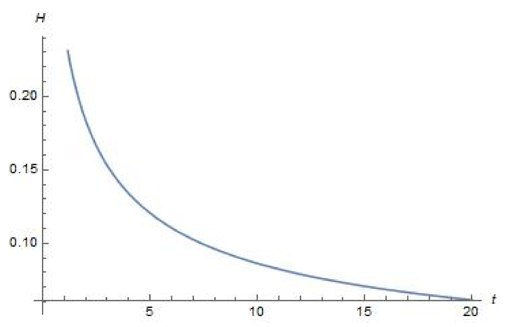
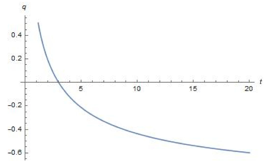
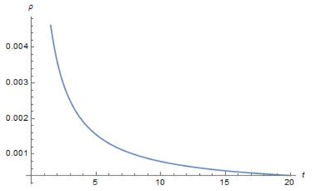
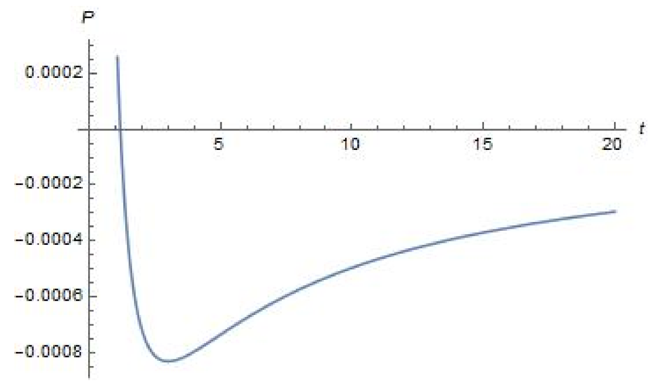
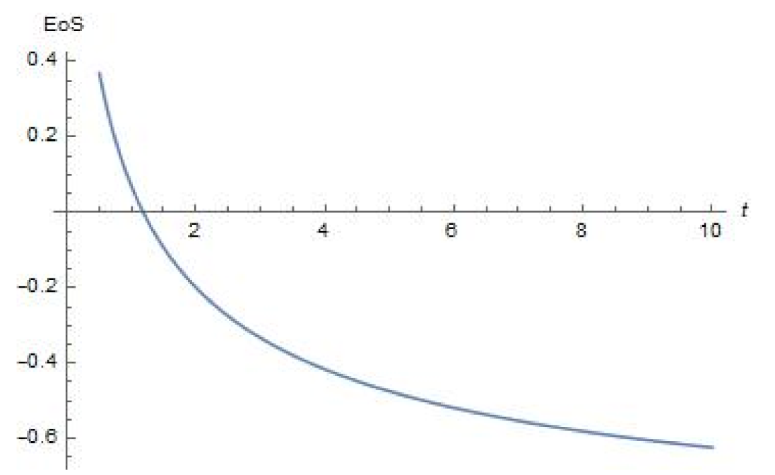
4. Plots of Parameters

In Figure 1 and Figure 2 below, we have plotted the the Hubble parameter H and deceleration parameter q against time:
The pressure, energy density and cosmological parameter and equation of state parameters are, respectively:
ρ = λ 1 ( 8 π + 2 λ 2 ) 3 + β λ 2 ( 8 π + λ 2 ) 2 β t + k 1 ( 2 β t + k ) ,
p = λ 1 ( 8 π + 2 λ 2 ) 3 + β ( 16 π + 3 λ 2 ) ( 8 π + λ 2 ) 2 β t + k 1 ( 2 β t + k ) ,
Λ = 3 λ 2 ( 8 π + 2 λ 2 ) β λ 2 ( 8 π + 2 λ 2 ) 2 β t + k 1 ( 2 β t + k ) ,
and
ω = 1 + β ( 16 π + 4 λ 2 ) 3 ( 8 π + λ 2 ) 2 β t + k + β λ 2 .
These parameters have been plotted against time in Figure 3, Figure 4, Figure 5 and Figure 6 below:

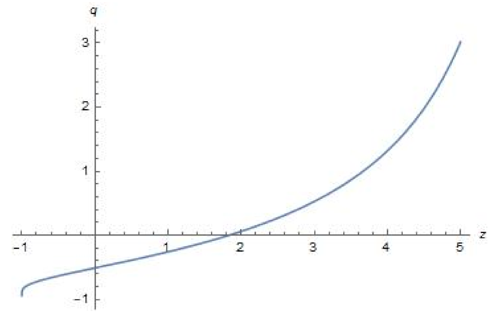
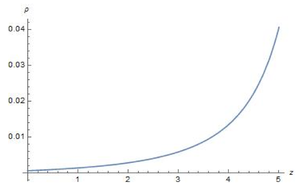
5. Parameters and Their Evolution in Terms of Redshift

From the observational point of view, it is preferable to express the parameters in term of redshift z. The scale factor a as a function of redshift is given by
a ( z ) = a 0 1 + z .
From Equation (32), we find
1 β 2 β t + k = l n ( a ) ,
and from Equation (38), we find
l n ( a ) = l n ( a 0 ) l n ( 1 + z ) .
Hence, the Hubble and deceleration parameters as functions of redshift are:
H ( z ) = 1 β [ l n ( a 0 ) l n ( 1 + z ) ] ,
q ( z ) = 1 + 1 [ l n ( a 0 ) l n ( 1 + z ) ] .
We now plot the deceleration parameter vs. redshift (Figure 7):
From this figure, it is easy to see that the deceleration parameter q was positive at early times, implying deceleration, and negative at late times, implying acceleration.
Using the t z relationship, we find the pressure, energy density, cosmological parameter and equation of state parameters as follows:
ρ = λ 1 ( 8 π + 2 λ 2 ) 3 + λ 2 ( 8 π + λ 2 ) [ l n ( a 0 ) l n ( 1 + z ) ] 1 β 2 [ l n ( a 0 ) l n ( 1 + z ) ] 2 ,
p = λ 1 ( 8 π + 2 λ 2 ) 3 + ( 16 π + 3 λ 2 ) ( 8 π + λ 2 ) [ l n ( a 0 ) l n ( 1 + z ) ] 1 β 2 [ l n ( a 0 ) l n ( 1 + z ) ] 2 ,
Λ = 3 λ 2 ( 8 π + 2 λ 2 ) λ 2 ( 8 π + 2 λ 2 ) [ l n ( a 0 ) l n ( 1 + z ) ] 1 β 2 [ l n ( a 0 ) l n ( 1 + z ) ] 2 ,
and
ω = 1 + ( 16 π + 4 λ 2 ) 3 ( 8 π + λ 2 ) [ l n ( a 0 ) l n ( 1 + z ) ] + λ 2 .
We can plot these quantities as follows (Figure 8, Figure 9, Figure 10 and Figure 11):

6. Energy Conditions

The material content of the universe must fulfil certain energy conditions. The weak energy condition (WEC), dominant energy condition (DEC) and strong energy condition (SEC) are given by, respectively:
ρ > 0 , ρ + p 0 ( W E C ) ,
ρ | p | ( D E C ) ,
ρ + 3 p 0 ( S E C ) .
These energy conditions can be plotted against time by making use of Equations (23) and (24).
From Figure 12 below, it can be seen that the matter content in this model obeys the W E C and D E C , but not the S E C , as to be expected. The S E C is violated at late times, as to be expected, since we need a negative pressure for late time accelerated expansion. However, at early times, the S E C is positive as required by big bang cosmology.

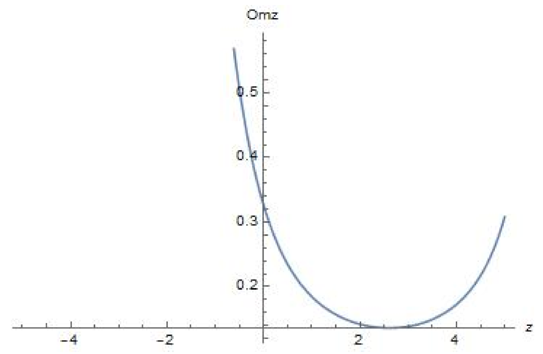
7. Om Diagnostic Analysis

There is a wide variety of models which are trying to reconstruct the properties of dark energy directly from observations. Such a procedure is very dependent on the priors assumed, such as the matter density, and the wrong choice for such priors can be problematic. The O m ( z ) diagnostic analysis is an attempt to distinguish the lambda cold dark matter model from competing ones with as few priors as possible [70]. It is known that all dark energy models needs a negative deceleration parameter q positive Hubble parameter H. Therefore, these parameters by themselves are not sufficient to distinguish amongst the variety of dark energy models available. The O m ( z ) analysis plays an important role in this regard. It has also been applied to the Galileo model [71,72]. The parameter O m ( z ) is defined by [73]:
O m ( z ) = [ H ( z ) H 0 ] 2 1 ( 1 + z ) 3 1 .
It can be seen that in the O m ( z ) equation, the first derivatives of the scale factor occur. For dark energy, a flat universe and constant equation of state ω , we find [70]
O m ( z ) = Ω m + ( 1 Ω m ) x α 1 x 3 1 ,
where Ω m is the matter density, x = 1 + z and α = 3 ( 1 + ω ) . From this, it can be seen that for the lambda cold dark matter model ( α = 0 ), O m ( z ) = Ω m , whilst for quintessence ( α > 0 ), O m ( z ) > Ω m and for the phantom case ( α < 0 ), O m ( z ) < Ω m . In the case of evolving dark energy models, where ω = ω ( z ) , the difference of the model from the standard lambda cold dark matter model is as follows: Quintessence is characterised by a concave upwards slope of O m ( z ) and phantom-type behaviour by a positive slope.
In our model O m ( z ) turns out to be:
O m ( z ) = 1 β 2 H 0 2 [ l n ( a 0 ) l n ( 1 + z ) ] 2 H 0 2 β 2 [ l n ( a 0 ) l n ( 1 + z ) ] 2 z ( 3 + 3 z + z 2 ) .
The function O m ( z ) is concave upwards, signifying a quintessence zone. We have plotted the graph of Om(z) in Figure 13 below, from which these characteristics are clearly visible.

8. Discussion

We have analysed the results of the theoretical calculations corresponding to our cosmological model against observational data. We found the values of the constants and k and β such that the present value of the deceleration parameter q 0 is 0.54 [74]. We used these values of β , k and λ in plotting all the figures.
In Figure 1, the variation of the Hubble parameter H is plotted against time t. We observe that the Hubble parameter H is a positive and decreasing function of the time t, and H 0 as t . Figure 2 plots the deceleration parameter against the time t. This graph affirms early deceleration and late-time acceleration. The transition occurs at q = 0 . In our model q 0.4 as t 0 and q 1 as t . In Figure 8, we plot the variation of q against z.
In Figure 3 and Figure 8, are plotted Equations (23) and (35), respectively, the energy density ρ against time t and redshift z, respectively. The energy density is a decreasing, positive function, and ρ 0 as t and z 1 , which is similar behaviour to the big-bang model. In Figure 4 and Figure 9, we have plotted the pressure p against time t and redshift z, as per Equations (24) and (36). We see that the pressure p is negative, corresponding to the current accelerating phase of the universe.
In Figure 5 and Figure 10, the cosmological parameter is plotted against time t and redshift z, respectively, (see Equations (25) and (37)). The cosmological parameter was large initially, is decreasing and Λ 0 as t (or z 1 ). This could help in resolving the cosmological constant problem [11], and a variable cosmological parameter could provide a better fit to observations [14]. In Figure 6 and Figure 11, the equation of state parameter is plotted against the time t and redshift z as per Equations (26) and (38), respectively. We notice that ω is not a constant but time dependent. The SNeIa data [75] limit ω to the range 1.67 < ω < 0.62 , while a combination of galaxy clustering statistics, SNeIa and CMB anisotropy data yield the range ω as 1.33 < ω < 0.72 . At present, our model exhibits quintessence with ω > 1 . Thus, our derived model is in keeping with observations [75,76,77].
Finally, in Figure 13, we have plotted O m ( z ) . Our model is presently in the quintessence zone ( ω > 1 ) , and will evolve into the phantom stage ( ω < 1 ) in future.

9. Conclusions

In this article, we have analysed a model containing a variable cosmological parameter in flat FLRW space-time in f ( R , T ) gravity by assuming a particular form of the deceleration parameter in terms of the Hubble parameter [78]. We graphed the various physical parameters against time, as well as redshift. The vital characteristics of our model are the following: Our model was decelerating in the past, and is currently accelerating as can be seen from Figure 2. The behaviour of the parameters q , ρ , p , ω , and Λ are illustrated by means of Figure 2, Figure 3, Figure 4 and Figure 5 and Figure 7, Figure 8, Figure 9 and Figure 10. We have a variable cosmological parameter, which was large initially, and which decreases with time. This could help in resolving the cosmological constant problem, and is a pleasing feature of f ( R , T ) gravity.
What can we say about the future of our model? As we can see from Equations (32), the model will continue to expand forever into the future. From the Equation (46) for the equation of state, as t , ω 1 , the lambda cold dark matter model. Hence, our model asymptotically tends to the lambda cold dark matter model in the future. With the values of the parameters that we have used, our equation of state parameter ω = 0.7 at z = 0 . This is somewhat higher than that inferred from observations [6], but it may be possible to attain a closer fit using different values for the parameters λ 1 and λ 2 . This is the subject of ongoing investigation, and we hope to report on this in the near future.

Author Contributions

Conceptualization, R.K.T., A.B., and B.K.S.; methodology, R.K.T.; software, A.B. and B.K.S.; validation, R.K.T., A.B. and B.K.S.; formal analysis, R.K.T., A.B. and B.K.S.; investigation, R.K.T., A.B. and B.K.S.; resources, R.K.T. and B.K.S.; data curation, B.K.S.; writing—original draft preparation, R.K.T. and B.K.S.; writing—review and editing, R.K.T., A.B., and B.K.S.; visualization, R.K.T., A.B., and B.K.S.; supervision, R.K.T. and A.B.; project administration, R.K.T.; funding acquisition, A.B. All authors have read and agreed to the published version of the manuscript.

Funding

This work is based on the research supported wholly/in part by the National Research Foundation of South Africa (Grant Numbers: 118511).

Institutional Review Board Statement

Not applicable.

Informed Consent Statement

Not applicable.

Data Availability Statement

Not applicable.

Acknowledgments

The authors are extremely grateful to the reviewers for their comments, which have substantially improved the article.

Conflicts of Interest

The authors declare no conflict of interest. The funders had no role in the design of the study; in the collection, analyses, or interpretation of data; in the writing of the manuscript, or in the decision to publish the results.

References

  1. Perlmutter, S.; Aldering, G.; Goldhaber, G.; Knop, R.A.; Nugent, P.G.; Castro, P.G.; Deustua, S.; Fabbro, S.; Goobar, A.; Groom, D.E.; et al. Measurements of Ω and Λ from 42 High-Redshift Supernovae. Astrophys. J. 1999, 517, 565–586. [Google Scholar] [CrossRef]
  2. Riess, A.G.; Filippenko, A.V.; Challis, P.; Clocchiatti, A.; Diercks, A.; Garnavich, P.M.; Gilliland, R.L.; Hogan, C.J.; Jha, S.; Kirshner, R.P.; et al. Observational Evidence from Supernovae for an Accelerating Universe and a Cosmological Constant. Astron. J. 1998, 116, 1009–1038. [Google Scholar] [CrossRef] [Green Version]
  3. Percival, W.J.; Baugh, C.M.; Bland-Hawthorn, J.; Bridges, T.; Cannon, R.; Cole, S.; Colless, M.; Collins, C.; Couch, W.; Dalton, G.; et al. The 2dF Galaxy Redshift Survey: The power spectrum and the matter content of the universe. Mon. Not. R. Astron. Soc. 2001, 327, 1297–1306. [Google Scholar] [CrossRef]
  4. Stern, D.; Jimenez, R.; Verde, L.; Kamionkowski, M.; Stanford, S.A. Cosmic chronometers: Constraining the equation of state of dark energy. I: H(z) measurements. J. Cosmol. Astropart. Phys. 2010, 1002, 008. [Google Scholar]
  5. Spergel, D.N.; Verde, L.; Peiris, H.V.; Komatsu, E.; Nolta, M.R.; Bennett, C.L.; Halpern, M.; Hinshaw, G.; Jarosik, N.; Kogut, A.; et al. First Year Wilkinson Microwave Anisotropy Probe (WMAP) Observations: Determination of Cosmological Parameters. Astrophys. J. Suppl. 2003, 148, 175–194. [Google Scholar] [CrossRef] [Green Version]
  6. Aghanim, N.; Akrami, Y.; Ashdown, M.; Aumont, J.; Baccigalupi, C.; Ballardini, M.; Banday, A.J.; Barreiro, R.B.; Bartolo, N.; Basak, S.; et al. Planck 2018 results VI. Cosmological parameters. Astron. Astrophys. 2020, 641, A6. [Google Scholar]
  7. Eisenstein, D.J.; Zehavi, I.; Hogg, D.W.; Scoccimarro, R.; Blanton, M.R.; Nicho, R.C.; Scranton, R.; Seo, H.; Tegmark, M.; Zheng, Z.; et al. Detection of the Baryon Acoustic Peak in the Large-Scale Correlation Function of SDSS Luminous Red Galaxies. Astrophys. J. 2005, 633, 560–574. [Google Scholar] [CrossRef]
  8. Sahni, V. The case for a positive cosmological Lambda-TERM. Int. J. Mod. Phys. D 2000, 9, 373. [Google Scholar] [CrossRef]
  9. Peebles, P.J.E.; Ratra, B. The Cosmological Constant and Dark Energy. Rev. Mod. Phys. 2003, 75, 559. [Google Scholar] [CrossRef] [Green Version]
  10. Bull, P.; Akrami, Y.; Adamek, J.; Baker, T.; Bellini, E.; Jimenez, J.B.; Bentivegna, E.; Camera, S.; Clesse, S.; Davis, J.H.; et al. Beyond ΛCDM: Problems, solutions, and the road ahead. Phys. Dark Univ. 2016, 12, 56–99. [Google Scholar] [CrossRef] [Green Version]
  11. Weinberg, S. The cosmological constant problem. Rev. Mod. Phys. 1989, 61, 1–23. [Google Scholar] [CrossRef]
  12. Babourova, A.; Frolov, B. The Solution of the Cosmological Constant Problem: The Cosmological Constant Exponential Decrease in the Super-Early Universe. Universe 2020, 6, 230. [Google Scholar] [CrossRef]
  13. Geng, C.; Lee, C.; Yin, L. Constraints on a running vacuum model. Eur. Phys. J. C 2020, 80, 69. [Google Scholar] [CrossRef]
  14. Sola, J. Cosmological constant vis-a-vis dynamical vacuum: Bold challenging the Lambda CDM. Int. J. Mod. Phys. A 2016, 31, 16300350. [Google Scholar] [CrossRef] [Green Version]
  15. Caldwell, R.R.; Dave, R.; Steinhardt, P.J. Cosmological Imprint of an Energy Component with General Equation of State. Phys. Rev. Lett. 1998, 80, 1582. [Google Scholar] [CrossRef] [Green Version]
  16. Singh, P.; Sami, M.; Dadhich, N. Cosmological dynamics of phantom field. Phys. Rev. D 2003, 68, 023522. [Google Scholar] [CrossRef] [Green Version]
  17. Sami, M.; Toporensky, A. Phantom field and the fate of the Universe. Mod. Phys. Lett. A 2004, 19, 1509. [Google Scholar] [CrossRef] [Green Version]
  18. Parker, L.; Raval, A. Nonperturbative effects of vacuum energy on the recent expansion of the universe. Phys. Rev. D 1999, 60, 063512. [Google Scholar] [CrossRef] [Green Version]
  19. Nojiri, S.; Odintsov, S.D. Quantum deSitter cosmology and phantom matter. Phys. Lett. B 2003, 562, 147–152. [Google Scholar] [CrossRef] [Green Version]
  20. Astashenok, A.V.; Nojiri, S.; Odintsov, S.D.; Yurov, A.V. Phantom cosmology without Big Rip singularity. Phys. Lett. B 2012, 709, 396. [Google Scholar] [CrossRef] [Green Version]
  21. Boyle, L.A.; Caldwell, R.R.; Kamionkowski, M. Spintessence! New models for dark matter and dark energy. Phys. Lett. B 2002, 545, 17. [Google Scholar] [CrossRef] [Green Version]
  22. Armendariz-Picon, T.; Mukhanov, V.F. k-Inflation. Phys. Lett. B 1999, 458, 209. [Google Scholar] [CrossRef] [Green Version]
  23. Chiba, T.; Okabe, T.; Yamaguchi, M. Kinetically driven quintessence. Phys. Rev. D 2000, 62, 023511. [Google Scholar] [CrossRef] [Green Version]
  24. Feng, B.; Wang, X.; Zhang, X. Dark Energy Constraints from the Cosmic Age and Supernova. Phys. Lett. B 2005, 607, 35. [Google Scholar] [CrossRef]
  25. Sen, A. Tachyon Matter. J. High Energy Phys. 2002, 0207, 065. [Google Scholar] [CrossRef] [Green Version]
  26. Padmanabhan, T. Accelerated expansion of the universe driven by tachyonic matter. Phys. Rev. D 2002, 66, 021301. [Google Scholar] [CrossRef] [Green Version]
  27. Khoury, J.; Weltman, A. Chameleon Fields: Awaiting Surprises for Tests of Gravity in Space. Phys. Rev. Lett. 2004, 93, 171104. [Google Scholar] [CrossRef] [Green Version]
  28. Chaplygin, S. On gas jets. Sci. Mem. Moscow Univ. Math. Phys. 1904, 21, 1–121. [Google Scholar]
  29. Copeland, E.J.; Sami, M.; Tsujikawa, S. Dynamics of dark energy. Int. J. Mod. Phys. D 2006, 15, 1753. [Google Scholar] [CrossRef] [Green Version]
  30. Sami, M.; Myrzakulov, R. Late time cosmic acceleration: ABCD of dark energy and modified theories of gravity. Int. J. Mod. Phys. D 2016, 25, 1630031. [Google Scholar] [CrossRef] [Green Version]
  31. Sami, M. Dark energy and possible alternatives. arXiv 2009, arXiv:0901.0756v1. [Google Scholar]
  32. Yoo, J.; Watanabe, Y. Theoretical models of dark energy. Int. J. Mod. Phys. D 2012, 21, 1230002. [Google Scholar] [CrossRef] [Green Version]
  33. Durrer, R.; Maartens, R. Dark Energy and Dark Gravity. Gen. Relativ. Grav. 2008, 40, 301–328. [Google Scholar] [CrossRef] [Green Version]
  34. Brax, P. What makes the Universe accelerate? A review on what dark energy could be and how to test it. Rep. Prog. Phys. 2018, 81, 016902. [Google Scholar] [CrossRef]
  35. Silvestri, A.; Trodden, M. Approaches to understanding cosmic acceleration. Rep. Prog. Phys. 2009, 72, 096901. [Google Scholar] [CrossRef] [Green Version]
  36. Tawfik, A.N.; El-Dahab, E.I. Review on Dark Energy Models. Grav. Cosm. 2019, 25, 103–115. [Google Scholar] [CrossRef]
  37. Harko, T.; Lobo, F.S.N.; Nokiri, S.; Odintsov, S.D. f(R,T) gravity. Phys. Rev. D 2011, 84, 024020. [Google Scholar] [CrossRef] [Green Version]
  38. Harko, T. Thermodynamic interpretation of the generalized gravity models with geometry-matter coupling. Phys. Rev. D 2014, 90, 044067. [Google Scholar] [CrossRef] [Green Version]
  39. Alvarenga, F.G.; de la Cruz-Dombriz, A.; Houndjo, M.J.S.; Rodrigues, E.; Saez-Gaomez, D. Dynamics of scalar perturbations in f(R,T) gravity. Phys. Rev. D 2013, 87, 103526. [Google Scholar] [CrossRef] [Green Version]
  40. Sharif, M.; Zubair, M. Energy conditions in f(R,T,RμνTμν) gravity. J. High Energy Phys. 2013, 12, 079. [Google Scholar] [CrossRef]
  41. Kiani, F.; Nozari, K. Energy conditions in F(T,Θ) gravity and compatibility with a stable deSitter solution. Phys. Lett. B 2014, 728, 554–561. [Google Scholar] [CrossRef] [Green Version]
  42. Alvarenga, F.G.; Houndjo, M.J.S.; Monwanou, A.V.; Chabi Orou, J.B.C. Testing some f(R,T) gravity models from energy conditions. J. Mod. Phys. 2013, 4, 130–139. [Google Scholar] [CrossRef] [Green Version]
  43. Sharif, M.; Zubair, M. Thermodynamics in f(R,T) Theory of Gravity. J. Cosmol. Astropart. Phys. 2012, 3, 28. [Google Scholar] [CrossRef] [Green Version]
  44. Jamil, M.; Momeni, D.; Ratbay, M. Violation of First Law of Thermodynamics in f(R,T) Gravity. Chin. Phys. Lett. 2012, 29, 109801. [Google Scholar] [CrossRef] [Green Version]
  45. Zubair, M.; Waheed, S.; Ahmad, Y. Static spherically symmetric wormholes in f(R,T) gravity. Eur. Phys. J. C 2016, 76, 444–457. [Google Scholar] [CrossRef] [Green Version]
  46. Moraes, P.H.R.S.; Sahoo, P.K. Modeling wormholes in f(R,T) gravity. Phys. Rev. D 2017, 96, 44038. [Google Scholar] [CrossRef] [Green Version]
  47. Moraes, P.H.R.S.; Correa, R.A.C.; Lobato, R.V. Analytical general solutions for static wormholes in f(R,T) gravity. J. Cosmol. Astropart. Phys. 2017, 7, 29. [Google Scholar] [CrossRef] [Green Version]
  48. Yousaf, Z.; Bamba, K.; Bhatti, M.Z.H. Causes of irregular energy density in f(R,T) gravity. Phys. Rev. D 2016, 93, 124048. [Google Scholar] [CrossRef] [Green Version]
  49. Moraes, P.H.R.S. Cosmological solutions from induced matter model applied to 5D f(R,T) gravity and the shrinking of the extra coordinate. Eur. Phys. J. C 2015, 75, 168–176. [Google Scholar] [CrossRef] [Green Version]
  50. Sahoo, P.K.; Sahoo, P.; Bishi, B.K. Anisotropic cosmological models in f(R,T) gravity with variable deceleration parameter. Int. J. Geom. Methods Mod. Phys. 2017, 14, 1750097. [Google Scholar] [CrossRef] [Green Version]
  51. Sahoo, P.K.; Sahoo, P.; Bishi, B.K.; Aygun, S. Magnetized strange quark model with Big Rip singularity in f(R,T) gravity. Mod. Phys. Lett. A 2017, 32, 1750105. [Google Scholar] [CrossRef] [Green Version]
  52. Perez, A.; Sudarsky, D. Dark energy as the weight of violating energy conservation. Phys. Rev. Lett. 2019, 118, 021102. [Google Scholar]
  53. Tiwari, R.K.; Beesham, A. Anisotropic model with decaying cosmological term. Astrophys. Space Sci. 2018, 363, 234. [Google Scholar] [CrossRef]
  54. Beesham, A.; Tiwari, R.K.; Shukla, B.K. Reconstruction of models with variable cosmological parameter in f(R,T) theory. In Proceedings of the 1st Electronic Conference on Universe, Basel, Switzerland, 22–28 February 2021; MDPI: Basel, Switzerland, 2021. [Google Scholar]
  55. Pasqua, A.; Chattopadhyay, S.; Khomenko, I. A reconstruction of modified holographic Ricci dark energy in f(R,T) gravity. Can. J. Phys. 2013, 91, 632–638. [Google Scholar] [CrossRef] [Green Version]
  56. Capozziello, S.; D’Agostino, R.; Luongo, O. Cosmographic analysis with Chebyshev. polynomials. Mon. Not. R. Astron. Soc. 2018, 476, 3924–3938. [Google Scholar] [CrossRef] [Green Version]
  57. Gruber, C.; Luongo, O. Energy conditions in f(Q,T) gravity. Phys. Rev. D 2014, 89, 103506. [Google Scholar] [CrossRef] [Green Version]
  58. Aviles, A.; Bravetti, A.; Capozziello, S.; Luongo, O. Dark degeneracy and interacting cosmic components. Phys. Rev. D 2014, 90, 043531. [Google Scholar] [CrossRef] [Green Version]
  59. de la Cruz-Dombriz, A.; Dunsby, P.K.S.A.; Luongo, O.; Reverberi, L. Model-independent limits and constraints on extended theories of gravity from cosmic reconstruction techniques. J. Cosmol. Astropart. Phys. 2016, 12, 042. [Google Scholar] [CrossRef] [Green Version]
  60. Zhou, Y.; Liu, D.; Zou, X.; Wei, H. New generalizations of cosmography inspired by the Pade approximant. Eur. Phys. J. C 2016, 76, 281. [Google Scholar] [CrossRef] [Green Version]
  61. Akarsu, O.; Dereli, T. Cosmological models with linearly varying deceleration parameter. Int. J. Theor. Phys. 2012, 51, 612–621. [Google Scholar] [CrossRef] [Green Version]
  62. Garg, P.; Zia, R.; Pradhan, A. Transit cosmological models in FRW universe under the two-fluid scenario. Int. J. Geom. Methods Mod. Phys. 2019, 16, 1950007. [Google Scholar] [CrossRef] [Green Version]
  63. Tiwari, R.K.; Beesham, A.; Shukla, B.K. Behaviour of the cosmological model with variable deceleration parameter. Eur. Phys. J. Plus 2016, 131, 447–456. [Google Scholar] [CrossRef]
  64. Tiwari, R.K.; Beesham, A.; Shukla, B.K. Cosmological models with viscous fluid and variable deceleration parameter. Eur. Phys. J. Plus 2017, 132, 20. [Google Scholar] [CrossRef]
  65. Tiwari, R.K.; Beesham, A.; Shukla, B.K. Scenario of a two-fluid FRW cosmological model with dark energy. Eur. Phys. J. Plus 2017, 132, 126. [Google Scholar] [CrossRef]
  66. Tiwari, R.K.; Beesham, A.; Shukla, B.K. Scenario of two-fluid dark energy models in Bianchi type-III Universe. Int. J. Geom. Methods Mod. Phys. 2018, 15, 1850155. [Google Scholar] [CrossRef]
  67. Tiwari, R.K.; Beesham, A.; Shukla, B.K. Cosmological model with variable deceleration parameter in f(R,T) modified gravity. Int. J. Geom. Methods Mod. Phys. 2018, 15, 1850189. [Google Scholar] [CrossRef]
  68. Jusus, J.F. Gaussian process estimation of transition redshift. J. Cosmol. Astropart. Phys. 2020, 4, 53. [Google Scholar] [CrossRef]
  69. Camarena, D.; Marra, V. Local determination of the Hubble constant and the deceleration parameter. Phys. Rev. Res. 2020, 2, 013028. [Google Scholar] [CrossRef] [Green Version]
  70. Sahni, V.; Shafieloo, A.; Starobinsky, A.A. Two new diagnostics of dark energy. Phys. Rev. D 2008, 78, 103502. [Google Scholar] [CrossRef] [Green Version]
  71. Jamil, M.; Momeni, D.; Myrzakulov, R. Wormholes in a viable f(T) gravity. Eur. Phys. J. C 2013, 73, 2347. [Google Scholar] [CrossRef]
  72. de Fromont, P.; de Rham, C.; Heisenberg, L.; Matas, A. Superluminality in the bi-and multi-Galileon. J. High Energy Phys. 2013, 7, 67. [Google Scholar] [CrossRef] [Green Version]
  73. Zunckel, C.; Clarkson, C. Consistency Tests for the Cosmological Constant. Phys. Rev. Lett. 2008, 101, 181301. [Google Scholar] [CrossRef] [PubMed] [Green Version]
  74. Giostri, R.; dos Santos, M.V.; Waga, I.; Reis, R.R.R.; Calvao, M.O.; Lago, B.L. From cosmic deceleration to acceleration: New constraints from SN Ia and BAO/CMBJ. J. Cosmol. Astropart. Phys. 2012, 3, 27. [Google Scholar] [CrossRef] [Green Version]
  75. Garnavich, P.; Jha, S.; Challis, P.; Clocchiatti, A.; Diercks, A.; Filippenko, A.V.; Gilliland, R.L.; Hogan, C.J.; Kirshner, R.P.; Leibundgut, B.; et al. Supernova Limits on the Cosmic Equation of State. Astrophys. J. 1998, 509, 74–79. [Google Scholar] [CrossRef] [Green Version]
  76. Nurbaki, A.N.; Capozziello, S.; Deliduman, C. Spherical and cylindrical solutions in f(T) gravity by Noether symmetry approach. Eur. Phys. J. C 2020, 80, 108–117. [Google Scholar] [CrossRef] [Green Version]
  77. Capozziello, S.; D’Agostino, R.; Luongo, O. Extended gravity cosmography. Int. J. Geom. Meth. Mod. Phys. 2019, 28, 1930016. [Google Scholar] [CrossRef] [Green Version]
  78. Tiwari, R.K.; Singh, R.; Shukla, B.K. A Cosmological Model with Variable Deceleration Parameter. Afr. Rev. Phys. 2015, 10, 48. [Google Scholar] [CrossRef]
Figure 1. Hubble parameter H (in G y r 1 ) against time t (in G y r ).
Universe 07 00319 g001
Figure 2. Deceleration parameter q against time t (in G y r ).
Universe 07 00319 g002
Figure 3. Energy density ρ (in G y r 2 ) against time t (in G y r ).
Universe 07 00319 g003
Figure 4. Pressure p (in G y r 2 ) against time t (in G y r ).
Universe 07 00319 g004
Figure 5. Cosmological parameter Λ (in G y r 2 ) against time t (in G y r ).
Universe 07 00319 g005
Figure 6. EOS parameter ω against time t (in G y r ).
Universe 07 00319 g006
Figure 7. Deceleration parameter q against redshift z.
Universe 07 00319 g007
Figure 8. Energy density ρ (in G y r 2 ) against redshift z.
Universe 07 00319 g008
Figure 9. Pressure p (in G y r 2 ) against redshift z.
Universe 07 00319 g009
Figure 10. Cosmological parameter Λ (in G y r 2 ) against redshift z.
Universe 07 00319 g010
Figure 11. Equation of state parameter ω against redshift z.
Universe 07 00319 g011
Figure 12. Energy conditions Ecs (in G y r 2 ) against time t (in G y r ) (green: ρ p ; r e d : ρ + p ; m a g e n t a : ρ + 3 p ).
Universe 07 00319 g012
Figure 13. Om diagnosis O m z against redshift z.
Universe 07 00319 g013
Publisher’s Note: MDPI stays neutral with regard to jurisdictional claims in published maps and institutional affiliations.

