Article

The Interplay between Canopy Structure and Topography and Its Impacts on Seasonal Variations in Surface Reflectance Patterns in the Boreal Region of Alaska—Implications for Surface Radiation Budget

Department of Geography and Environmental Science, Hunter College of the City University of New York, New York, NY 10021, USA
*
Author to whom correspondence should be addressed.
Remote Sens. 2021, 13(16), 3108; https://doi.org/10.3390/rs13163108
Submission received: 28 June 2021 / Revised: 29 July 2021 / Accepted: 31 July 2021 / Published: 6 August 2021
(This article belongs to the Special Issue Remote Sensing Applications for Land Surface Properties and Processes)

Abstract

:
Forests play an essential role in maintaining the Earth’s overall energy balance. The variability in forest canopy structure, topography, and underneath vegetation background conditions create uncertainty in modeling solar radiation at the Earth’s surface, particularly for boreal regions in high latitude. The purpose of this study is to analyze seasonal variation in visible, near-infrared, and shortwave infrared reflectance with respect to land cover classes, canopy structures, and topography in a boreal region of Alaska. We accomplished this investigation by fusing Landsat 8 images and LiDAR-derived canopy structural data and multivariate statistical analysis. Our study shows that canopy structure and topography interplay and influence reflectance spectra in a complex way, particularly during the snow season. We observed that deciduous trees, also tall with greater rugosity, are more dominant on the southern slope than on the northern slope. Taller trees are typically seen in higher elevations regardless of vegetation types. Surface reflectance in all studied wavelengths shows similar relationships with canopy cover, height, and rugosity, mainly due to close connections between these parameters. Visible and near-infrared reflectance decreases with canopy cover, tree height, and rugosity, especially for the evergreen forest. Deciduous forest shows more considerable variability of surface reflectance in all studied wavelengths, particularly in March, mainly due to the mixing effect of snow and vegetation. The multivariate statistical analysis demonstrates a significant tree shadow effect on surface reflectance for evergreen forests. However, the topographic shadow effect is prominent for deciduous forests during the winter season. These results provide great insight into understanding the role of vegetation structure and topography in surface radiation budget in the boreal region.

1. Introduction

Forests play a critical role in regulating the world’s climate and maintaining the Earth’s overall energy balance [1]. The forest canopies often show high structural complexity (known as “rugosity”, [2]). In particular, conifer forests exhibit a complex canopy structure [3] and tree shadowing effects, altering surface reflectance spectra and the surface radiation budget against different background conditions, resulting in varying air temperatures. Complex vegetation structure induces considerable uncertainty in estimating and modeling the Earth’s radiation budget [4] because incoming solar radiation interacts with vegetation canopies through complex canopy radiative transfer processes [5].
Forest canopy reflectance is a function of various factors, including leaf optical properties, canopy structures, background conditions, solar illumination geometries, the viewing angles, and the topography, e.g., elevation [3,6,7,8,9,10]. The presence of snow on the ground or the leaves and branches adds complexity to forest canopy reflectance due to its high reflectivity, especially in the visible and near-infrared wavelengths [11,12]. The forest canopy structures interact in snow accumulation and disappearance mechanisms because trees and canopy structures intercept and attenuate solar radiation [13,14,15]. In [13], it was demonstrated that a heterogeneous vegetation structure induces wide spatial variation in snow accumulation and persistence. The highly reflective snow makes a heterogeneous surface mixed with absorbent forest canopies, particularly in visible wavelengths. Under these circumstances, the overall reflectivity of the surface reduces considerably compared with forest-free snow-covered surfaces [16]. Such behavior also contributes to the more significant spatial heterogeneity in the snow melting processes, as forest canopy density can control melt rates [10]. Topography presents a further challenge in rugged terrains to understand the role of complex vegetation structures in surface reflectance and surface albedo at different spectrums [17,18].
The knowledge of vertical and horizontal forest structures is essential in understanding incoming solar radiation’s surface radiative processes interacting with vegetation and the forest floor [19]. The large variability in forest structures can modulate the generation of shades and exert variation in snow accumulation and snowmelt conditions [13]. The accurate assessment of the relationship between vertical or horizontal forest structure and surface reflectance is essential for the quantitative measurement and modeling of the solar radiation budget. Radiative transfer (RT) models were developed to simulate the physics of radiative transfer processes. Nevertheless, many RT models assume the homogeneous canopy and leaf area index (LAI) to be the only structure inputs, not considering other vegetation structures. Other models, such as geometric optical and radiative transfer theory (GORT), integrate structural information. However, the GORT models often require detailed vegetation structure inputs. These vegetation structure inputs are readily available across large spatial scales [20,21], and it is hard to simulate spatial variability. Therefore, detailed specifics of canopy structural information are necessary for accurate modeling and quantification [22]. Combining optical data from the moderate resolution and more extensive geographic coverage Landsat satellites with high-resolution 3D vegetation-structure parameters from LiDAR (light detection and ranging) would not only address spatio-temporal heterogeneities of surface radiative processes associated with gaps and edges within a forest stand but also allows us to identify direct relationships between vegetation structure measurements by LiDAR with the seasonal multispectral surface reflectance measured by Landsat.
In boreal forests, forest floor conditions can affect canopy reflectance because it constitutes heterogeneous and clumped forest canopies [23,24]. The seasonal snow that overlaps a significant portion of the boreal forests in the northern hemisphere creates seasonal variations in snow accumulation and snowmelt conditions [16,23]. The above-described state constitutes a significant challenge to accurately investigating the impact of complex vegetation structure on surface reflectance at different spectrums in these areas. The availability of satellite-derived optical data forms a cost-effective option for obtaining information on the Earth’s radiation budget and finding relationships between vegetation structure observation and surface radiation. Additionally, remote sensing data can provide valuable information on the interaction between vegetation and incoming solar radiation on a continuous spatial and temporal scale because remote sensing data provide fewer limitations and uncertainties than modeled parameters.
Therefore, this study investigates the relationship between canopy structures, topography, and surface reflectance in visible, near-infrared, and shortwave infrared wavelengths during different seasons in a boreal forest near Fairbanks, Alaska, by combining Landsat 8 images and LiDAR-derived canopy metrics. We explored the causes of variations in visible, near-infrared, and shortwave infrared reflectance during different seasons concerning LiDAR-derived canopy metrics, such as tree heights, rugosity (i.e., structural complexity), and canopy cover and topography (slope, elevation, and aspect). The accurate understanding of the effect of complex forest structure on visible, near-infrared, and shortwave infrared reflectance in snow-dominated rugged terrain will guide us on how best to fuse the global vegetation structure measured by the Global Ecosystem Dynamics Investigation (GEDI) mission with climate prediction models. The canopy radiative transfer model embedded in climate models could effectively simulate the impact of vegetation structure on land surface reflectance at global scales [21].

2. Materials and Methods
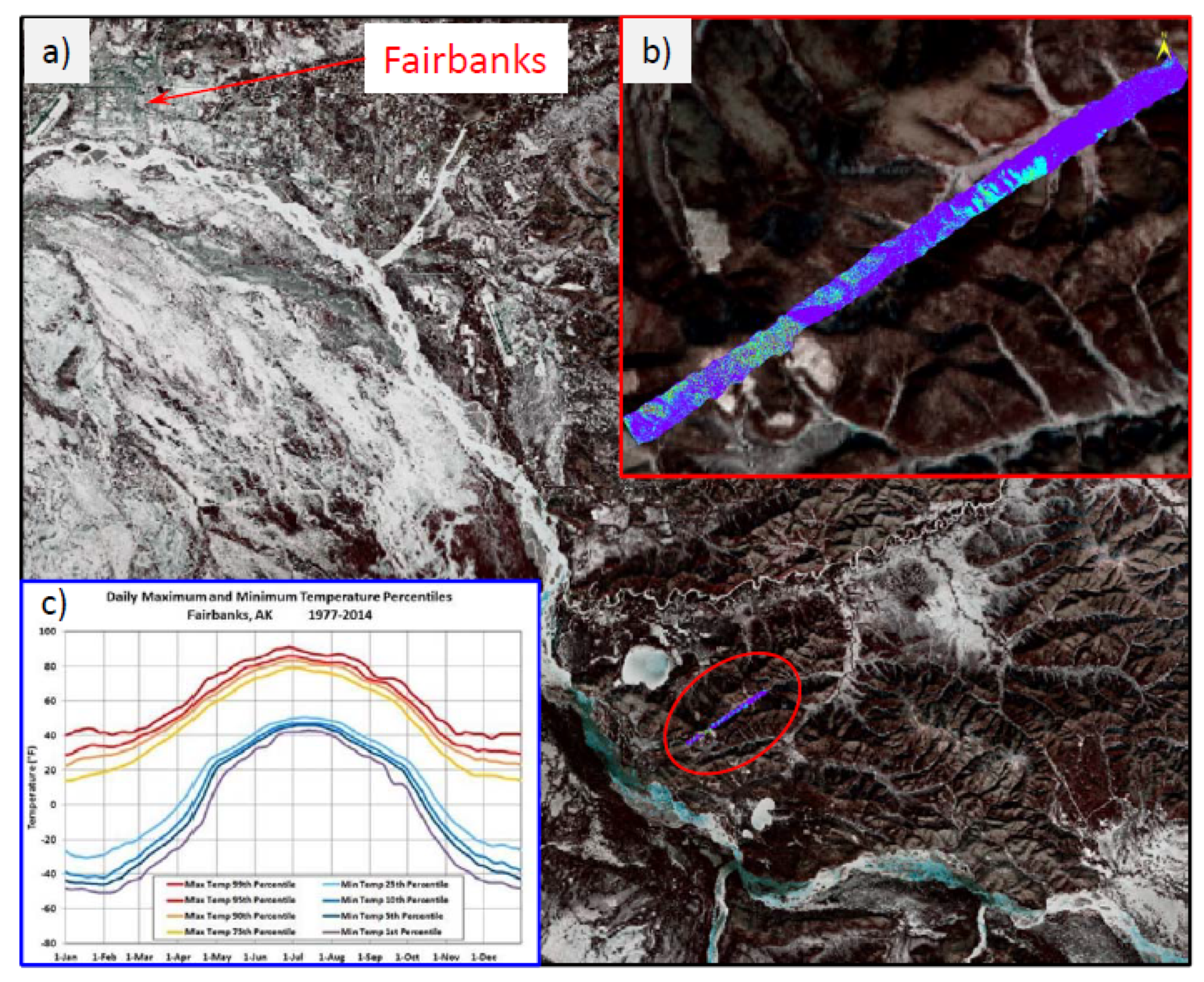
2.1. Study Area

The study area falls within the Level-III ecoregion of Alaska. The site is bordered by Interior Highlands and Interior Bottomlands ecoregions and is in a mountainous area near the Harding-Birch lakes region in Fairbanks, Alaska (Figure 1). The study area is approximately 400 m wide and 8000 m long, and the shape is elongated in the NE-SW direction. The topography is highly variable and is located in the central Tanana valley. The elevation ranges between 350 and 600 m above mean sea level, with slopes ranging between 0 and 30 degrees. The vegetation communities include spruces, firs, conifers, and deciduous trees along waterways [25]. The site is dominated by evergreen (white spruce: Picea glauca and black spruce: Picea mariana species) and deciduous (e.g., paper birch: Betula papyrifera species) forests.
The study area experiences a continental subarctic climate with mild summers and icy winters. It has four seasons, including short summer (average high temperature of 22.8 °C with a high in July) and dominant winter season (average low temperature of −27.2 °C with a low in January). The average annual snowfall is 1651 mm, which lasts from October to May and peaks in January.

2.2. Data

Landsat 8 OLI/TIRS (Operational Land Imager/Thermal Infrared Sensor) surface reflectance (Band 3—Green: 0.53–0.59 μm, Band 5—Near-Infrared: 0.85–0.88 μm, and Band 6—Shortwave Infrared: 1.57–1.65 μm) of 30 m spatial resolution was used in this study. The images were downloaded from U.S. Geological Survey (USGS) Earth Explorer data portal. Detailed product information can be downloaded from the USGS website [26]. Satellite images from three time periods, 26 March, 29 May, and 8 August 2014, were selected for this study. The date of scenes was determined based on cloud-free conditions and to observe seasonal patterns.
We downloaded LiDAR data from NASA’s G-LiHT program [27]. LiDAR data were acquired on 6 August 2014, overlapping one of the Landsat 8 scenes we chose to study. We used several LiDAR metrics, such as mean tree return heights (tree_mean), quadratic mean tree return heights (tree_qmean), the standard deviation of tree return heights (tree_stdev), the standard deviation of gridded canopy height model (tree_rugosity), the fraction of first returns intercepted by the tree (tree_fcover), and the fraction of all returns classified as a tree (tree_fract_all). The data is at 13 m spatial resolution. In addition, we used slope, aspect, and elevation derived from the gridded digital terrain model.
The National Land Cover Database (NLCD) 2011 [28] at 30 m spatial resolution was used to identify the dominant land cover classes in the study area. The land cover classes were determined based on the assumption that the trees in each category were taller than 5 m and consisted of more than 20% of the total canopy cover. In addition to that, more than 75% of the tree species in deciduous forests lose foliage in response to seasonal changes. In contrast, more than 75% of the tree species in the evergreen forest class maintain foliage all year. We identified two main land cover classes (i.e., deciduous and evergreen forests) in the study area.

2.3. Methodology

Landsat 8 surface reflectance from visible, near-infrared, and shortwave infrared wavelength regions from three time periods were co-registered with LiDAR-derived vegetation metrics and NLCD 2011 land cover datasets. Landsat surface reflectance and NLCD land cover classes were resampled at the 13 m spatial resolution to correspond with LiDAR metrics. Pixel-level (n = 4574) information was extracted in ArcGIS Pro 2.8.1 (ESRI Inc.) for detailed statistical analysis in RStudio 4.0.4 software.
We compared seasonal variation of Landsat 8 surface reflectance in two NLCD 2011 land cover classes (i.e., deciduous and evergreen forests). We then examined the relationships of LiDAR metrics (e.g., canopy cover, tree heights, and rugosity) and topography (e.g., elevation, slopes, and aspects) with surface reflectance in three wavelength regions.
The coefficient of variation (CV) was calculated to evaluate the effects of land cover classes on surface reflectance in different wavelength regions in the study area.
C V = σ | μ | ×   100 %
where σ and μ are the standard deviation and the mean of the surface reflectance corresponding to different wavelengths and land cover classes. A higher CV indicates more significant variability and thus shows stronger effects.
Ordinary least square (OLS) regression analysis using multiple independent variables was carried out to quantify the relationship of canopy metrics and topography variables with surface reflectance in winter (March) and summer (August) scenes for visible and near-infrared bands.
y = β 0 + β 1 X i + β 2 X j + + β n X n + ε
where Y is the predicted variable, Xi-n is the explanatory variable, β0 is the intercept, β1-n is the slope of the relationship between Xi-n (multiple independent variables) and Y, and ε is the error.
The OLS regression is well known for its simplicity and has good predictive power [29]. The analysis was conducted in R environments using the olsrr package [30]. The best model was chosen using the ols_step_best_subset function of the olsrr package and based on the larger adjusted R-squared and the smaller Akaike information criterion (AIC) [31].
The relationship between response (surface reflectance) and predictor (LiDAR-derived canopy metrics and topography) variables exhibited a complex non-linear pattern, mainly due to the heterogeneity in environmental conditions. Therefore, a non-linear model was constructed using the Generalized Additive Models (GAM). The GAM is a widely used model in ecological studies and can fit complex, non-linear functions between predictor and response variables [32,33].
Z = β 0 + i = 1 N s i ( X i )
where β0 is the intercept, si(Xi) is the smooth function of Xi (the predictor variables), Z is the predicted (response) variable.
We used mgcv’s gam package in R environments, which offers several different methods for selecting smoothing parameters and basis functions [34]. The mgcv’s “Restricted Maximum Likelihood” method was used in this analysis. The technique offers default smooth and basis functions and provides reliable and stable results. The final GAM model was selected based on the significance of influential predictors, the lower AIC, and the higher adjusted R-square. The model was evaluated by analyzing Q-Q plot, histogram of residuals, and response versus fitted values that followed a pattern clustered around the 1-to-1 line.

3. Results

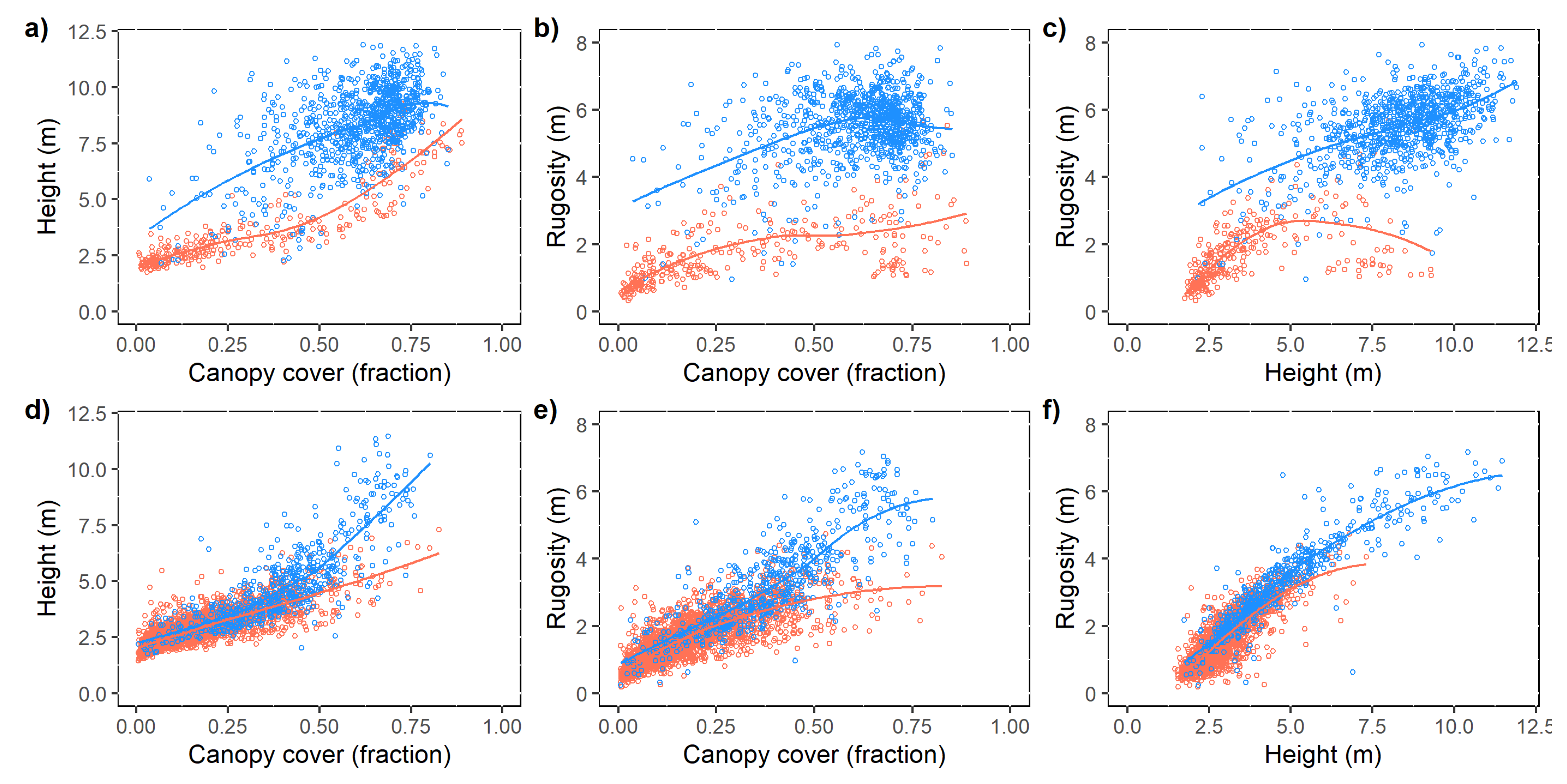
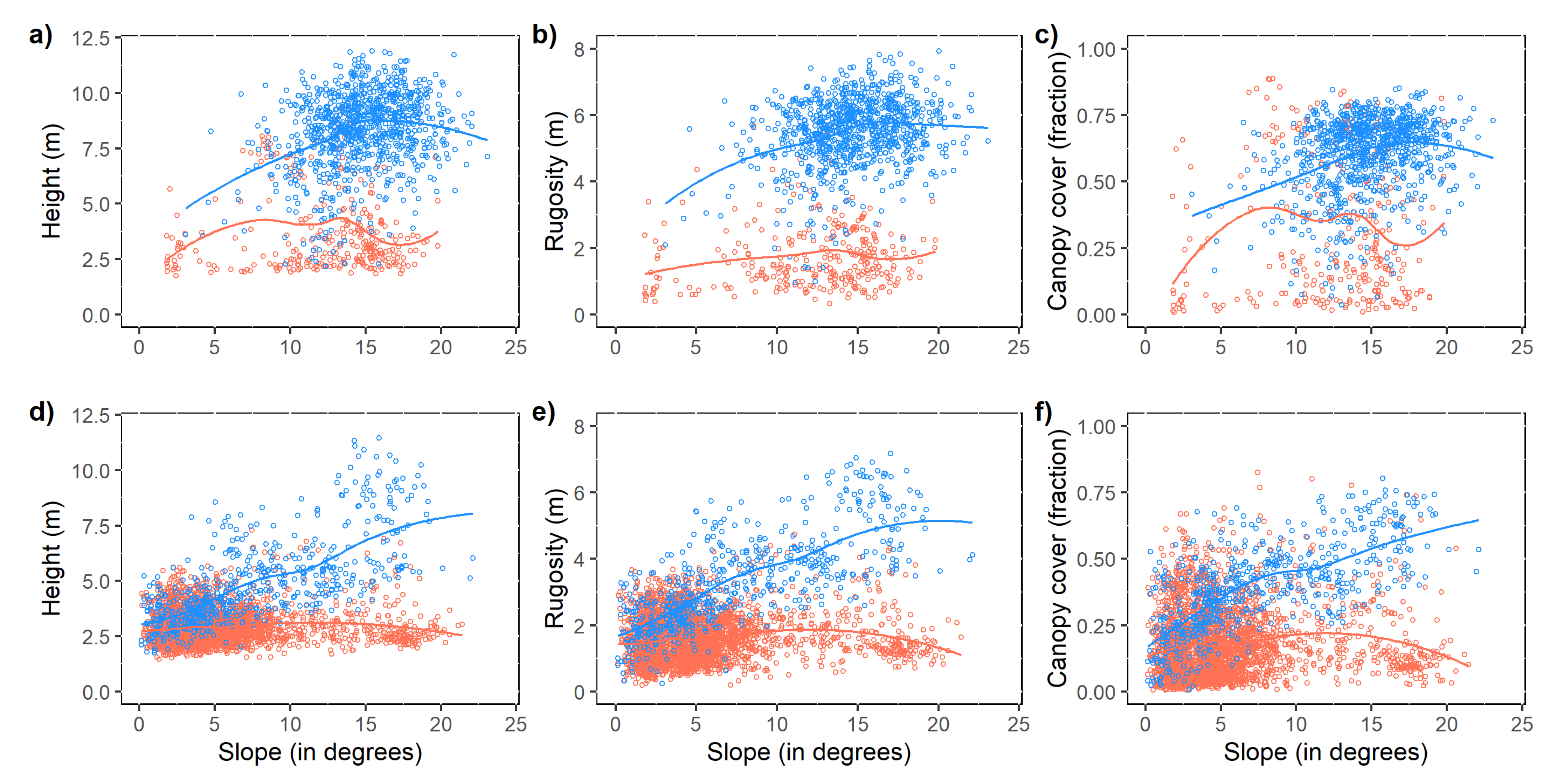
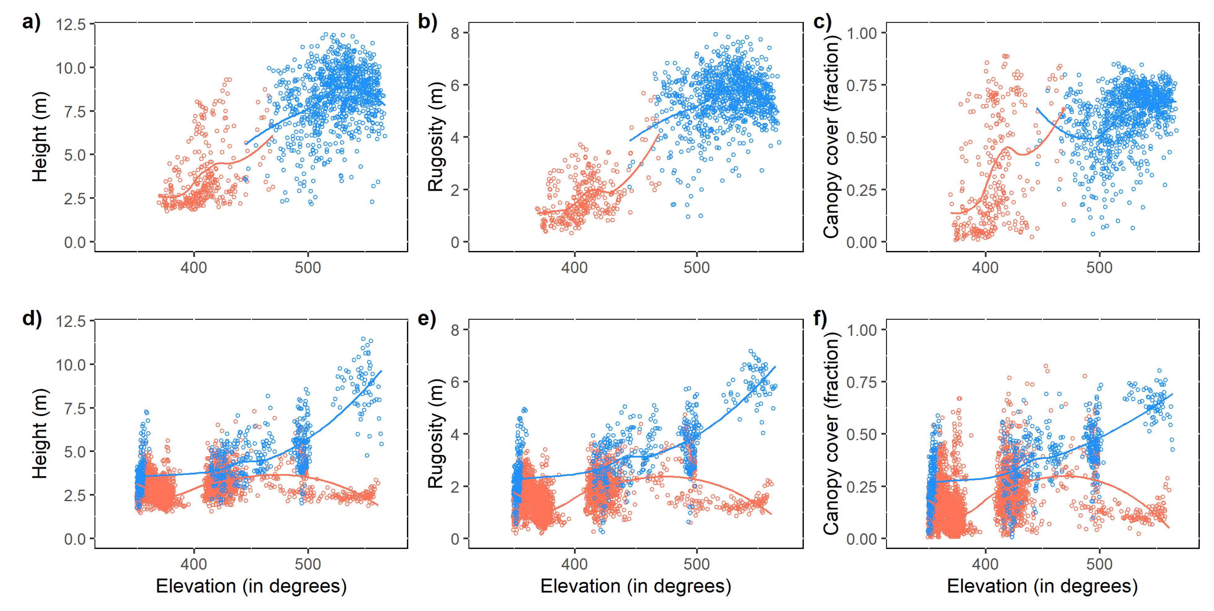
3.1. Relationship between Canopy Structure, Topography, and Land Cover Types

We observed significantly higher canopy cover in deciduous forests during the leaf-on season than the evergreen forests (mean canopy cover fraction of 0.54 and 0.21, respectively). Likewise, trees were taller in deciduous forests than in evergreen forests (mean heights of 7.2 m and 3.2 m, respectively). The height variability (rugosity) was more prominent in deciduous forests than in evergreen forests (mean rugosity of 4.6 m and 1.9 m, respectively). Deciduous forests were dominant in the southern aspect; trees tend to be taller with more height variability and more canopy cover than evergreen forests. On the other hand, evergreen forests were evenly distributed in both southern (between 90 and 270 degrees) and northern (>270 degrees and <90 degrees) aspects. However, evergreen forests in the southern aspect tend to be taller with more height variability.
The relationship between canopy cover and tree heights is non-linear for deciduous and evergreen forests (Figure 2). The locally weighted scatterplot smoothing (LOWESS) regression line shows different intercepts for trees in northern and southern aspects in deciduous forests, suggesting different minimum tree heights (Figure 2a). The LOWESS regression lines show similar intercepts in evergreen forests; however, with increasing canopy cover, the increase in tree heights is much more significant in southern aspects than in northern aspects (Figure 2d). The correlation between canopy cover and rugosity is non-linear for deciduous and evergreen forests (Figure 2b,e). Likewise, the correlation between tree heights and rugosity is non-linear (Figure 2c,f). The trend in the LOWESS regression line is different for deciduous forests in northern and southern aspects. On the other hand, the LOWESS regression line follows the same path for trees <5 m and canopy cover <0.40 in both aspects in evergreen forests.
We further investigated the relationship between canopy structures and topography (such as slopes, elevation, and aspect) (Figure 3). Evergreen forests are primarily located on low slopes (mean slope of 5.7°), whereas deciduous forests are mainly located on high slopes (mean slope of 14°). Tree height, rugosity, and canopy cover increase with the increase in slopes (Figure 3). However, tree height remains unchanged with an increase in slopes in northern aspects. On the other hand, taller trees with higher rugosity and more canopy cover dominate southern aspects.
We observed increasing tree height, rugosity, and canopy cover with an increase in elevation, but the rate of change is more significant in southern aspects than in northern aspects (Figure 4). In deciduous forests, trees are clustered in two groups, one in low elevation and the other in high elevation. Still, these trees show a positive change in heights, rugosity, and canopy cover with elevation (Figure 4a–c). While for evergreen forests, this trend only works for trees in the southern aspect (Figure 4d–f). However, canopy structure metrics do not show any relationship with elevation on the northern slope.

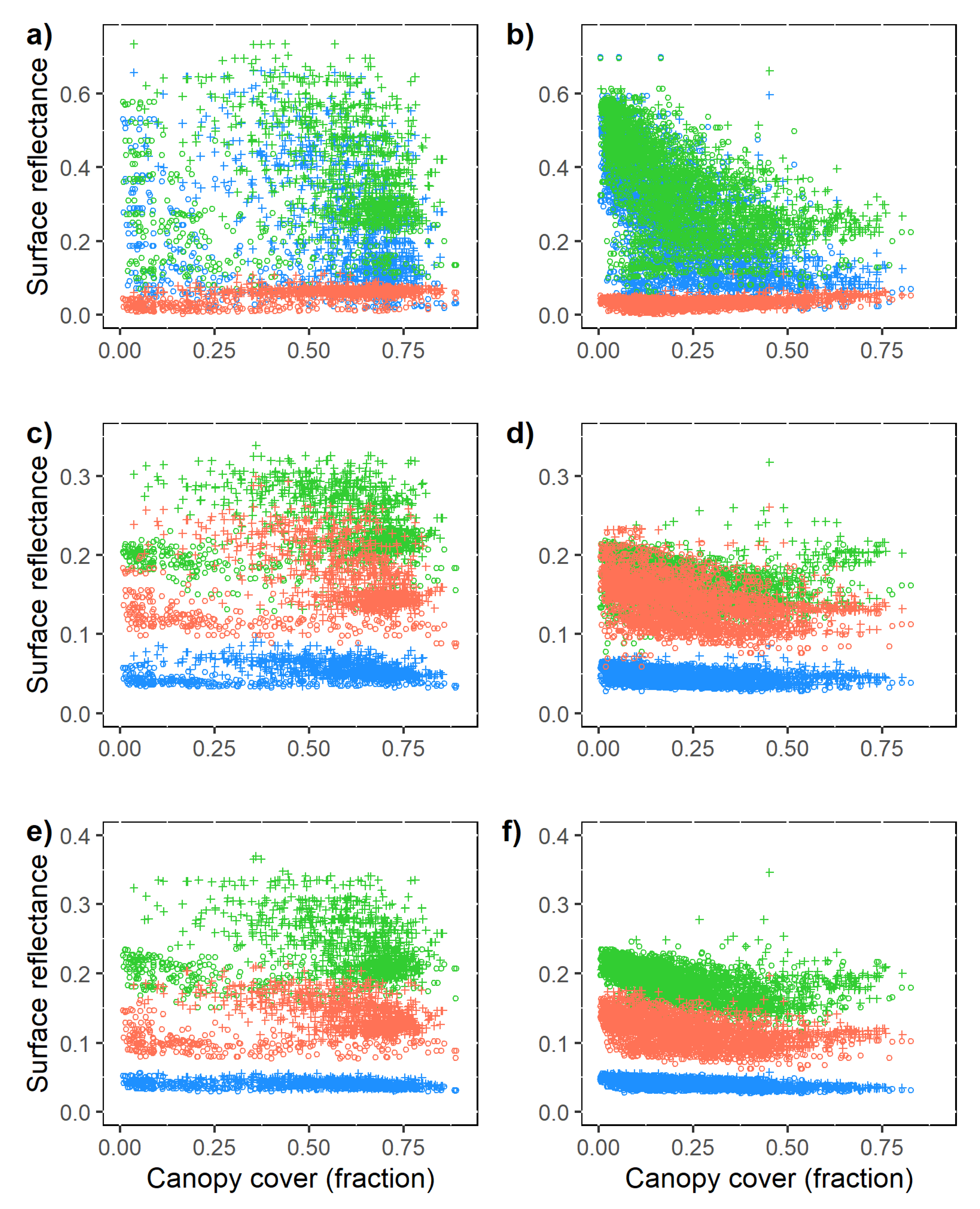
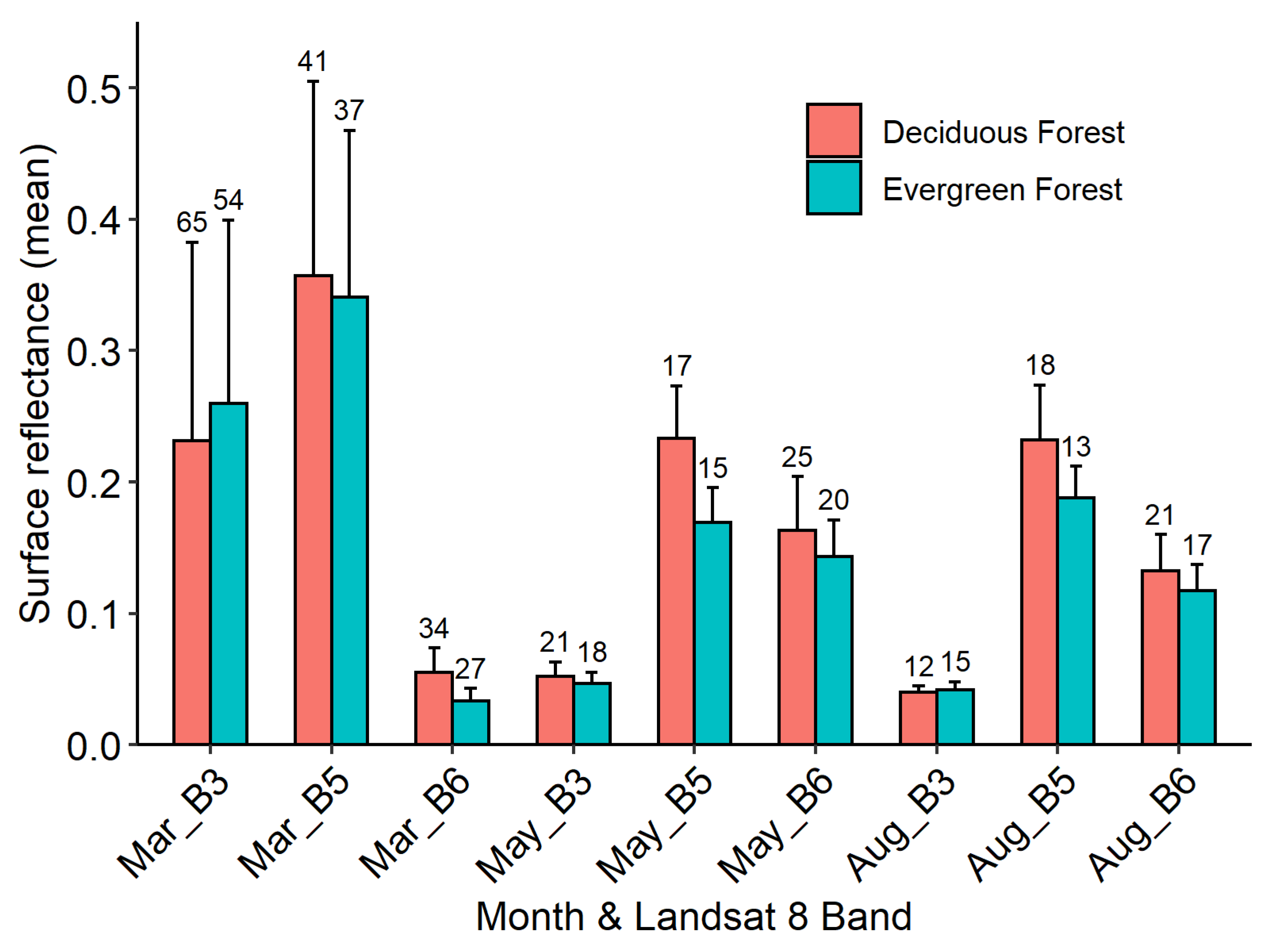
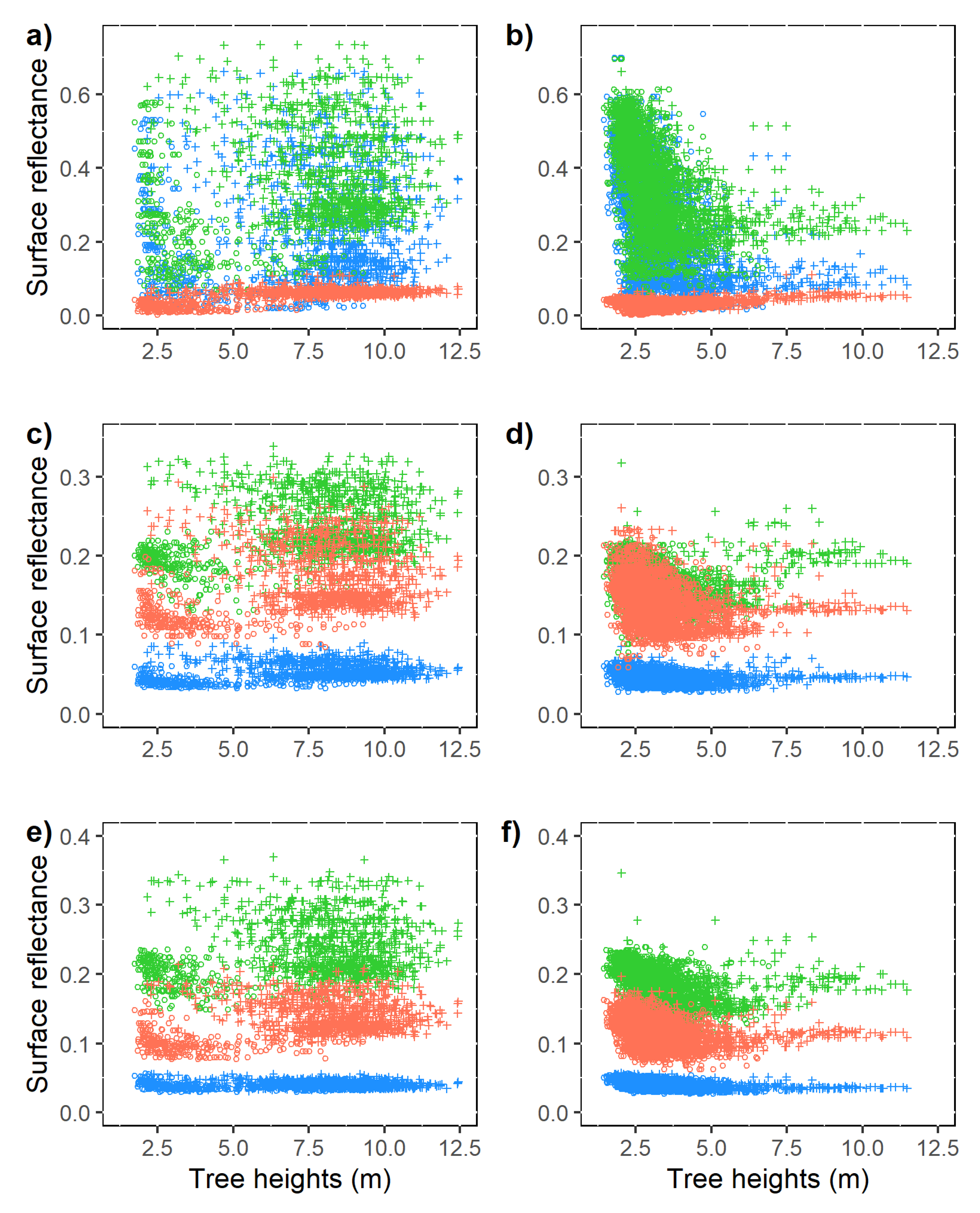
3.2. Land Cover Types, Canopy Structures, and Surface Reflectance Pattern

Surface reflectance in visible (Band 3, 0.53–0.59 μm), near-infrared (Band 5, 0.85–0.88 μm), and shortwave infrared (Band 6, 1.57–1.65 μm) spectrums were shown for deciduous and evergreen land cover classes during March, May, and August 2014 (Figure 5). Surface reflectance in visible wavelengths was the highest in March, followed by May and August. Near-infrared reflectance was the highest in March, followed by August and May, whereas shortwave infrared reflectance was the highest in May, followed by August and March. The coefficient of variations (CVs) was the highest in March, whereas CVs were similar in May and August (Figure 5). However, during March, visible wavelengths (Band 3) have slightly lower surface reflectance than near-infrared wavelengths (Band 5). During winter, the variation in surface reflectance could have resulted from large-scale surface heterogeneity created by snow accumulation, as indicated by higher CVs in visible bands (54 to 65%) than the near-infrared bands (37 to 41%).
In evergreen forests, the visible and near-infrared reflectance decreases with increasing canopy cover during different months (Figure 6b,d,f). The magnitude of this decrease is much greater in March than in other months. These results imply a significant masking effect of boreal evergreen forest on surface reflectance. However, in March, shortwave infrared reflectance increases with an increase in canopy cover, which could be due to higher solar radiation absorption at these wavelengths by snow at lower canopy cover, while at higher canopy cover, lesser solar radiation absorption could be due to more significant masking effects. In deciduous forests, the trees are clustered into two groups, one group with higher canopy cover fractions, the other with lower canopy cover fractions (Figure 6a,c,e). Deciduous forest shows more considerable variability in surface reflectance in all three wavelength regions, particularly in March, mainly due to the mixing effect of snow and vegetation. Large variabilities of surface reflectance in visible and near-infrared spectrums suggest heterogeneity in masking effect by the branches during leaf-off seasons. Surface reflectance does not show a particular pattern within each group with changes in canopy cover fractions (Figure 6a,c,e). For similar canopy cover, the evergreen forest has lower surface reflectance than deciduous forest, irrespective of wavelengths and seasons. It is partially because the deciduous forest is a dominant vegetation type in the southern aspect. It may also be due to the more substantial masking effect caused by tree shadowing in evergreen forests during the snow season. Considerable variability in surface reflectance during different months and LC classes with respect to canopy cover suggests multiple controlling factors such as tree heights and rugosity, which has a non-linear relationship with canopy cover in our study area.
Surface reflectance in all studied wavelengths shows similar relationships with canopy cover, height, and rugosity, mainly due to close connections between these three parameters (Figure 2). The results show a significant change in visible and near-infrared reflectance for evergreen forests when tree heights change from 2 to 5 m (Figure 7b). Evergreen forests show much lower surface reflectance in visible and near-infrared wavelengths than the deciduous forests when tree heights were more than 5 m, particularly in the March scene. The above result suggests a more significant masking effect by trees in the evergreen forest than the deciduous forest on snow surface reflectance (Figure 7a,b). During the leaf-off season (i.e., winter and early spring), deciduous forests cast more gaps than evergreen forests, allowing the impact from background snow on surface reflectance in the visible and near-infrared spectrum. At the same time, taller trees in evergreen forests could produce more shade and lower the reflectance in the visible and near-infrared wavelengths. In shortwave infrared bands, a slight increase in surface reflectance with increased tree heights could be due to a lack of absorption by the snow, especially in March (Figure 7). In contrast, higher shortwave infrared reflectance in May and August than in March for shorter tree heights could be due to a lack of soil moisture and leaf water content. With increasing tree heights, the effect of snow and moisture content diminishes. This condition is more pronounced during May and August than the March scene.
The relationship between surface reflectance and rugosity is similar to the relationship between surface reflectance and tree height (Figure 8). Generally, taller forests with maximum canopy heights have higher rugosity [35]. We observed a decreasing trend of surface reflectance in visible, near-infrared, and shortwave infrared bands with increasing rugosity during different months of the year for both LC classes (Figure 8). Higher surface reflectance at low rugosity could be attributed to less scattering of lights at the canopy level. In addition to that, snow-covered surfaces produce higher surface reflectance than bare soil surfaces. Therefore, the chances of background effects increase during winter when trees are less variable in heights. The figure shows two clusters of trees in deciduous forests, one with low and the other with high rugosity (Figure 8a,c,e). These clusters show declining trends in surface reflectance of all bands with increasing rugosity, especially in May and August.

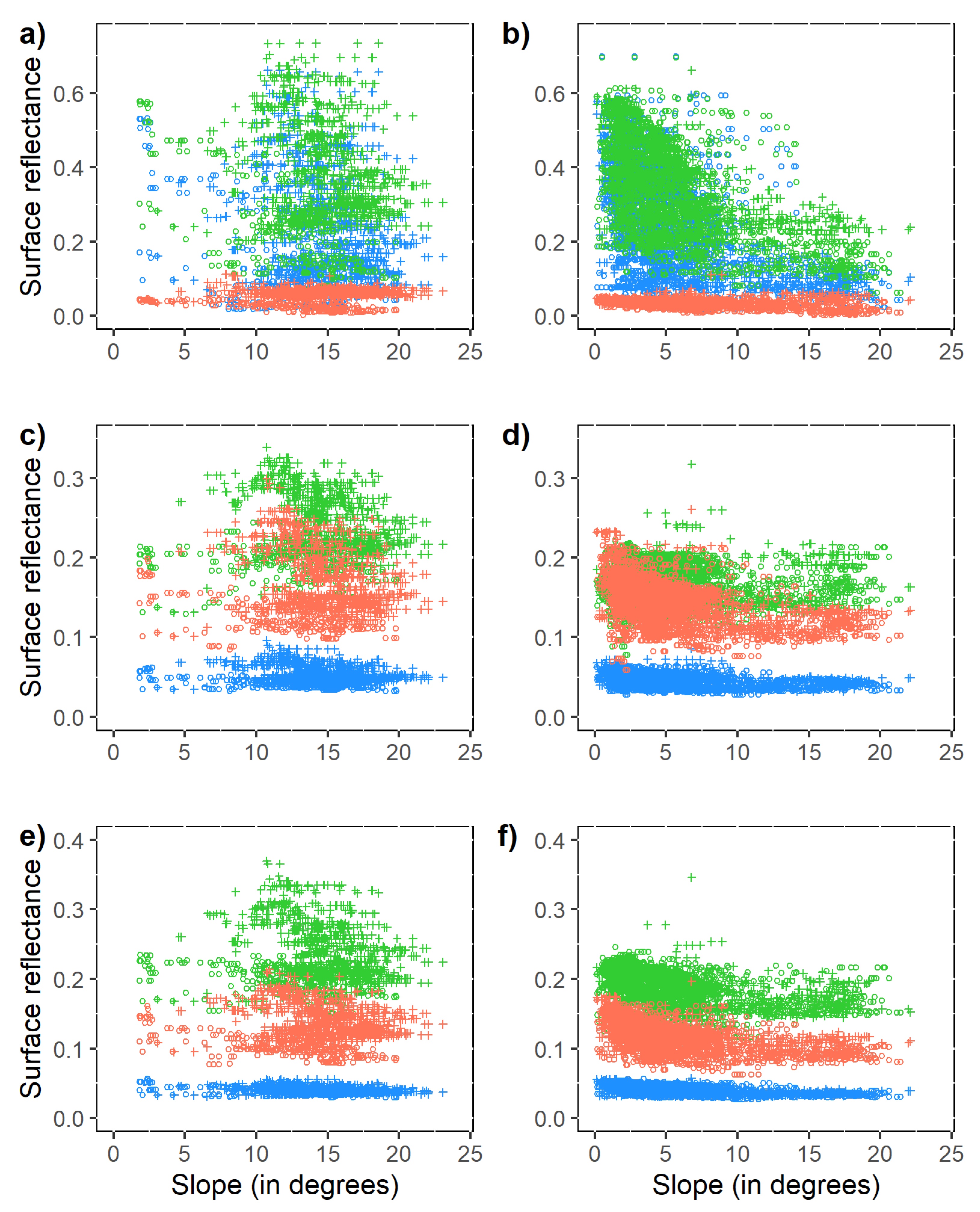
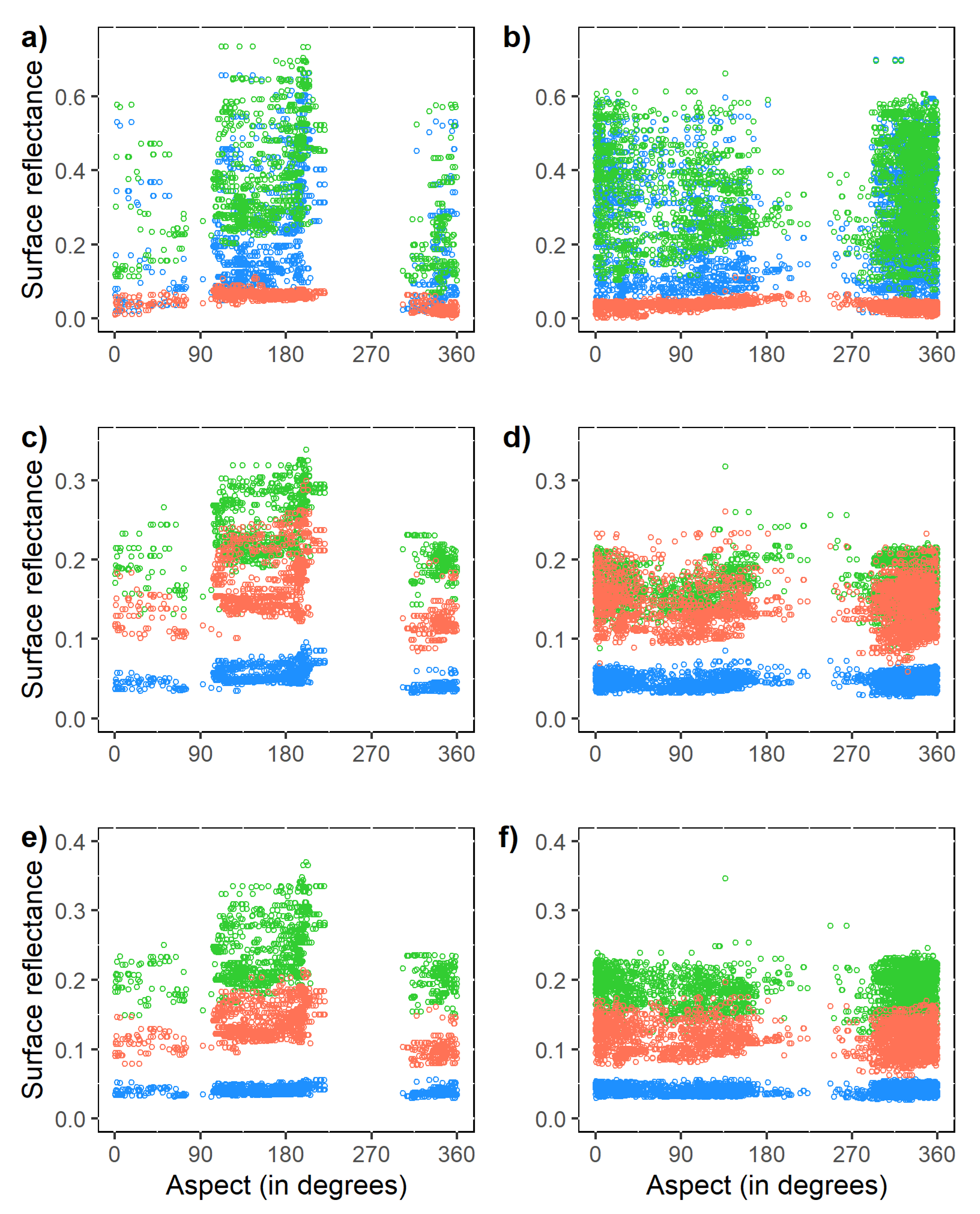
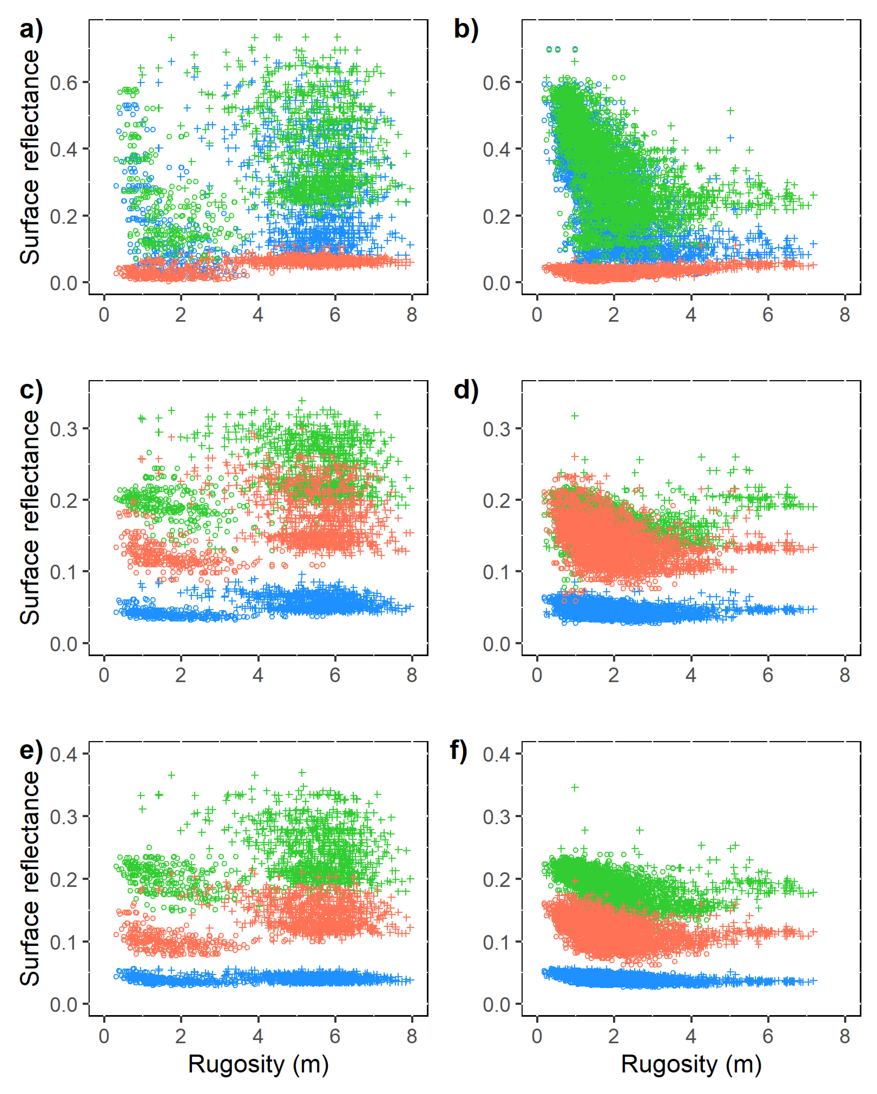
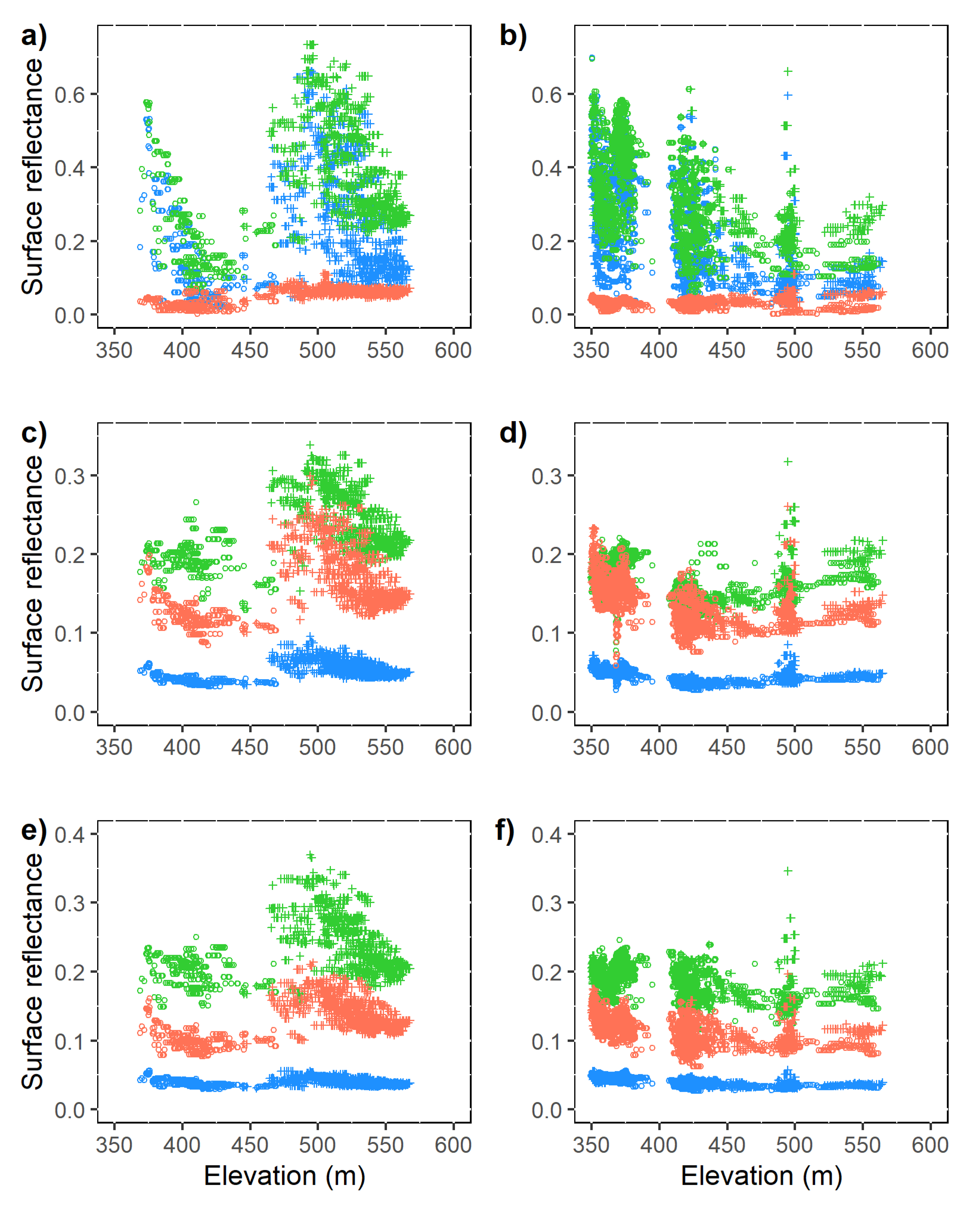
3.3. Surface Reflectance as a Function of Topography

Surface reflectance in all wavelengths decreases with increased slopes and is less variable at higher slopes, especially in evergreen forests (Figure 9). In evergreen forests, the mean surface reflectance in all wavelengths was much higher at slopes <10°. This result is consistent with a higher share of shorter trees with less height variability in lower slopes than in higher slopes and negligible tree shadowing effect. On the contrary, more shadows and absorption of solar radiation were observed in the region with taller trees with more height variability on high slopes. A similar trend was also observed for trees in deciduous forests, but trees are typically on higher slopes than evergreen forests. We observed more variability of surface reflectance, especially in visible and near-infrared wavelengths, in both land cover classes during March. In May and August, the change in surface reflectance was small for both LC classes. Such a large change in surface reflectance values during March could be attributed to the differences in the level of snow accumulation and melting rates on different slopes [36]. In addition, the variability in surface reflectance in the studied wavelengths could also increase due to masking effects by trees in evergreen forests and branches during leaf-off conditions in deciduous forests.
There is a decreasing trend of surface reflectance in the studied wavelength regions with an increase in elevation in evergreen forests (Figure 10b,d,f). Likewise, the two tree clusters in deciduous forests show declining surface reflectance with an increase in elevation (Figure 10a,c,e). This result is consistent with the findings that tree heights, rugosity, and canopy cover increase with elevation (Figure 4). However, such relationships are much more distinct for trees located in the southern aspects. The close relationship between elevation and surface reflectance in each studied wavelength is related to what was observed before, i.e., taller and denser trees distributed in higher elevation produce more absorption of solar radiation. The less noisy relationship between surface reflectance and elevation, compared to canopy cover, tree heights, and rugosity (Figure 6, Figure 7 and Figure 8), indicates an integrated effect of tree height, rugosity, and canopy cover on surface reflectance.
As expected, the relationship between surface reflectance (in three wavelength regions) and aspect shows an interesting pattern (Figure 11). For deciduous forests, higher surface reflectance in the southern aspect than the northern slope indicates a stronger shadow effect due to topography on the northern slope; even the trees are shorter and less covered in the northern slope. For evergreen forests, surface reflectance is primarily independent of aspects (Figure 10b,d,f), suggesting that the shadow effects from tree crowns on surface reflectance are more significant, especially during March.

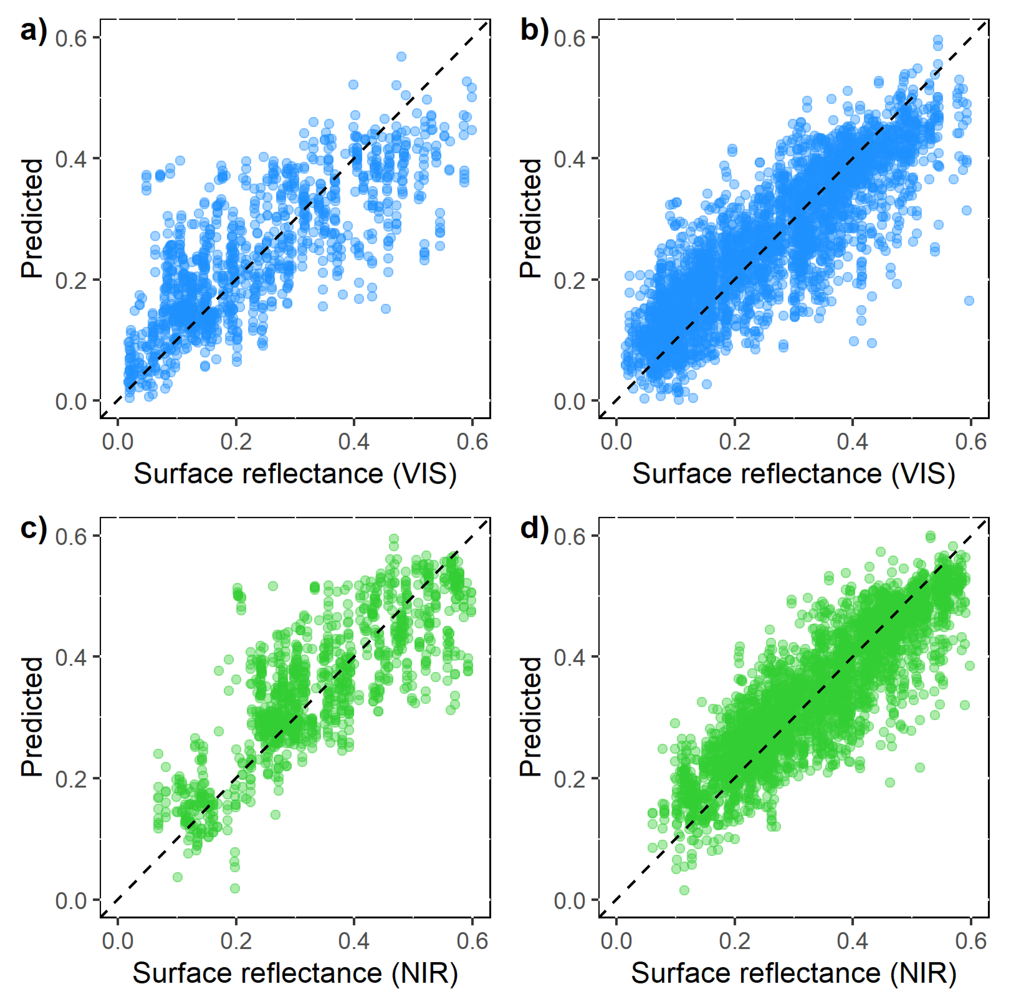
3.4. Contribution of Topography and Canopy Structure on Surface Reflectance Pattern

We show topography impacts on vegetation growth and its structure. Surface reflectance in three studied wavelengths is sensitive to change in slope, elevation, canopy cover, tree height, and rugosity. The variability of surface reflectance is much higher in the deciduous forest when trees are on low slopes with low elevation, which produces shorter, insignificant height differences and less canopy cover. On the other hand, surface reflectance in evergreen forests is not highly sensitive to change in topography and canopy structures. The higher sensitivity at shorter heights and rugosity could be attributed to reflectance from the snow-covered ground surfaces in March. In May and August, reflectance from the ground surface (including understory vegetation) can contribute to the overall sensitivity. As the height, rugosity, slope, and elevation increase, the decrease in sensitivity could be attributed to more solar radiation absorption at the canopy level [37].
The multivariate OLS regression revealed that slope and canopy cover alone could explain 50% and 56%, respectively, of the variance in visible and near-infrared reflectance for the March scene of evergreen forests. The OLS model derived adjusted R-squared values were 0.50 and 0.56, respectively. However, we observed a significant improvement in the model prediction and explained variance when we considered a non-linear function through the GAM approach (Table 1). The GAM model explained between 74% and 76% of the visible and near-infrared reflectance variance, respectively, by canopy cover, rugosity, slope, elevation, and aspects. It is important to note that GAM model showed that elevation and canopy cover alone could explain approximately 40% of the variance in the data (Table 1). For deciduous forests, topographic variables (slope, elevation, and aspect) alone explained 42% and 52% of the visible and near-infrared reflectance variance, respectively, in the March scene based on multivariate OLS regression. The OLS model derived adjusted R-squared values of 0.42 and 0.52, respectively. On the other hand, the GAM based on non-linear relationships between predictor and response variables explained between 60% and 68% of the variance in surface reflectance of visible and near-infrared bands, respectively, for the same scene. Such a relationship confirms that the topography plays a dominant role in the variation in surface reflectance from visible and near-infrared bands in deciduous forests. In contrast, tree shadow dominantly controls surface reflectance in evergreen forests. Predicted surface reflectance in visible and near-infrared bands for the March scene based on GAM approach shows a good model fit with most data points clustered around 1-to-1 line of observed versus predicted values (Figure 12).
For the August scene (summer season), the OLS regression model explained the contribution of canopy cover and slope in near-infrared reflectance but with a lesser degree, adjusted R-squared value of 0.35 for evergreen forests, while the effect of topography (i.e., slope, aspect, and elevation) remained dominant for deciduous forests with the OLS regression model, which explained 43% of the variance of near-infrared reflectance. When the non-linearity term through the GAM approach was introduced into the model, the adjusted R-squared values improved compared to the OLS regression model (Table 1). The comparison of the models showed that GAM models effectively explained the data for both March and August scenes better than OLS models. However, the GAM model was slightly more effective in explaining visible and near-infrared reflectance during winter for deciduous and evergreen forests. Such a difference could be attributed to the differences in surface conditions (such as snow on the ground, leaves, and branches) and the change in solar zenith angle.

4. Discussion

In all studied wavelengths, the mean surface reflectance (except for the Green band in March) and coefficient of variation (except for the Green band in August) are slightly higher in the deciduous forest than in the evergreen forest. During the snow season, deciduous forests lose foliage in response to seasonal changes. Such conditions allow satellites to see more background and produce higher surface reflectance than the evergreen forests, which maintain foliage all year. The more significant variation in surface reflectance in the visible and near-infrared region of the electromagnetic (EM) spectrum indicates greater differences in surface heterogeneity in March than in May and August for both forest types. Such heterogeneity is typically associated with differences in snow accumulation and melting rates in boreal regions due to the large variability in tree structures, which were also observed in our study area [13]. In [12], higher variability in surface reflectance in the presence of snow layers during winter was observed. In addition, evergreen forests (conifers) have much more absorptive capacity than deciduous forests [7]. The role of background reflectance from snow-covered surfaces is confirmed by observing the highest mean and broader range of surface reflectance in March for both visible and near-infrared bands compared to those in May and August for both LC classes, while the reflectance from shortwave infrared bands in March was lower than in May and August due to high absorption by snow and snowmelt on the ground. Such a variation in surface reflectance during different months and throughout the ranges of the EM spectrum is consistent with creating a highly heterogeneous surface due to differential accumulation and melting rates of highly reflective snow in the study area. The presence of snow and canopy covers that are highly absorptive surfaces for incoming solar radiation likely produces a broader range of surface reflectance in March [16]. The results further indicate that the variation in surface reflectance in our study during different seasons is controlled in part by the land cover classes [38] together with snow-vegetation interactions and the creation of heterogeneous surfaces.
The non-linear relationships of canopy cover with tree height and rugosity have a significant implication when assessing the impact of vegetation structure on surface reflectance and albedo. Our analysis indicates that canopy cover alone is insufficient to explain the variability in surface reflectance due to the saturation issue. Thus, tree height and rugosity (height variability) are important vegetation structure parameters. In [39], it was observed that canopy rugosity is positively correlated to the fraction of photosynthetically active radiation and primary production under high light conditions. These relationships indicate that surface topographic characteristics control vegetation structure characteristics at the landscape scale in addition to local climatic conditions. Elevation and aspect (slope orientation) are two critical factors determining vegetation types, height, and rugosity, which affect surface reflectance at stand scale. Our non-linear modeling effort confirms the finding that in addition to canopy cover, tree height and rugosity also affect surface reflectance and albedo [1,40,41]. Generally, higher canopy structural complexity is associated with more light absorption and thus greater photosynthesis and vegetation growth [35,37]. The close association between canopy cover, tree height and rugosity, and correlation with surface reflectance in the studied wavelengths imply an inherent relationship between structure and surface reflectance. This has been modeled using the geometric optical and radiative transfer (GORT) theory [8,21].
In [42], it has been indicated that variable topography could have resulted in uneven tree growth due to a lack of soil moisture and nutrient availability. This might be attributed to the observed canopy structural complexity (i.e., the variations in tree heights and rugosity) in relation to slopes and elevation in both forest types. In deciduous forests, the observed higher surface reflectance in visible and near-infrared wavelengths with higher variability in the southern aspects than in the northern aspects could be due to the shadowing effect by topography. On the other hand, shorter and less variable trees in evergreen forests suggest vegetation growth is independent of aspects. Our results, namely, that there is higher reflectance on the southern slope (backward scattering) than on the northern slope (forward scattering) agree well with the results derived from bidirectional reflectance distribution function (BRDF) spectral reflectance models [43]. In [43], the progress of BRDF modeling over rugged terrains was reviewed. They found that the canopy reflectance increased in the backward direction while decreasing in the forward direction with the increase in slope. In [44], the effects of slope and aspects on the variability of daily solar radiation have been indicated. The slope could result in spatial heterogeneity in vegetation structure and composition [45]. Our final GAM model confirmed the contribution of canopy structures (such as tree height, rugosity, and canopy cover) and added complexity due to topography (slope, elevation, and aspect) in controlling visible and near-infrared reflectance in the study area.
This research has some limitations. The study area is small and thereby lacks applicability to a larger area of different land cover classes, a range of canopy metrics, and different topography. The forests in the studied region are highly diverse. Therefore, applying the knowledge gained from this study to a larger area is an important step forward in climate research. The non-linear relationships between surface reflectance (visible and near-infrared bands) and independent variables used in the GAM’s approach needed a detailed assessment. Such relationships could be effectively addressed using machine learning techniques to interpret the effect of snow cover and tree/topographic shadows. We will implement the knowledge gained from this study to a much larger area and enable the fusion of high-resolution LiDAR measurements with Landsat surface reflectance and albedo estimates. We will also conduct a time-series analysis by adding more scenes that will allow us to understand temporal patterns and seasonality.

5. Conclusions

Our study suggests that canopy structure and topography interplay and influence surface reflectance in a complex way, particularly during the snow season. First, we found that topographic aspects and elevation influence vegetation type and structure distribution. The southern slope of our study region is dominated by deciduous forests with taller trees and denser canopy cover than evergreen forests. At the same time, evergreen forests are evenly distributed on both southern and northern slopes, with taller trees and more considerable height variability on the southern slope than on the northern slope. Taller and denser trees are located at higher elevations on the southern slope. On the northern slope, vegetation structures do not show any relationship with elevation.
Surface reflectance in visible, near-infrared, and shortwave infrared wavelengths shows similar relationships with canopy cover, height, and rugosity, mainly due to the close connection between these parameters. The decrease in visible and near-infrared reflectance with increasing canopy cover, tree height, and rugosity, especially for the evergreen forest, is consistent with the canopy radiative transfer modeling results. Deciduous forest shows considerable variability in visible and near-infrared reflectance, particularly in March, mainly due to the mixing effect of snow and vegetation.
The relationship between vegetation structure and surface reflectance is significantly impacted by topography. The topographic aspect controls vegetation growth and vegetation types, such as deciduous forests, which are dominant in the southern aspect, thus further constituting taller trees with greater rugosity than the northern aspect. Elevation also controls vegetation metrics; for example, higher elevation is associated with taller trees from both vegetation types, particularly in the southern aspect. Thus, vegetation structure and surface topography form a complex relationship and affect surface reflectance on a hierarchical scale. At a larger scale, surface topography (elevation, slope, and aspect) forms specific vegetation structure characteristics. While, at a finer scale, vegetation heterogeneity (canopy cover, height, and rugosity) combined with larger scale shadowing effect due to topography effect on surface reflectance pattern. Our study suggests that the shadow effect from topography and tree crowns on surface reflectance plays a different role in deciduous and evergreen forests. For evergreen forests, surface reflectance is primarily independent of aspects, suggesting that the tree shadow plays a prominent effect on surface reflectance, especially during March. In contrast, for deciduous forests, the topographic shadow effect is significant. Our study suggests that accurate modeling of surface reflectance and surface radiation budget would require detailed vegetation structure and topography inputs in the model.

Author Contributions

Conceptualization and Methodology, B.N. and W.N.-M.; Software, Formal Analysis and Data Curation, B.N.; Writing—Original Draft Preparation, B.N.; Writing—Review and Editing, B.N. and W.N.-M.; Funding Acquisition, W.N.-M. Both authors have approved the content of the published version of the manuscript.

Funding

This study is funded by NASA grant number 80NSSC20K1718.

Institutional Review Board Statement

Not applicable.

Informed Consent Statement

Not applicable.

Data Availability Statement

Landsat 8 OLI/TIRS surface reflectance data product at 30 m spatial resolution can be ordered freely at https://earthexplorer.usgs.gov/ (accessed on 1 December 2020). LiDAR data product can be downloaded from https://glihtdata.gsfc.nasa.gov/ (accessed on 1 December 2020). National Land Cover Database 2011 can be downloaded from https://www.mrlc.gov/ (accessed on 1 December 2020).

Acknowledgments

The authors would like to thank anonymous reviewers for their time and effort in reviewing this paper and improve this paper’s quality.

Conflicts of Interest

The authors declare no conflict of interest.

References

  1. Alibakhshi, S.; Naimi, B.; Hovi, A.; Crowther, T.W.; Rautiainen, M. Quantitative analysis of the links between forest structure and land surface albedo on a global scale. Remote Sens. Environ. 2020, 246, 111854. [Google Scholar] [CrossRef]
  2. Hardiman, B.S.; Bohrer, G.; Gough, C.M.; Vogel, C.S.; Curtis, P.S. The role of canopy structural complexity in wood net primary production of a maturing northern deciduous forest. Ecology 2011, 92, 1818–1827. [Google Scholar] [CrossRef] [PubMed] [Green Version]
  3. Kötz, B.; Schaepman, M.; Morsdorf, F.; Bowyer, P.; Itten, K.; Allgöwer, B. Radiative transfer modelling within a heterogeneous canopy for estimation of forest fire fuel properties. Remote Sens. Environ. 2004, 92, 332–344. [Google Scholar] [CrossRef]
  4. Myneni, R.B.; Ramakrishna, R.; Nemani, R.; Running, S.W. Estimation of global leaf area index and absorbed par using radiative transfer models. IEEE Trans. Geosci. Remote Sens. 1997, 35, 1380–1393. [Google Scholar] [CrossRef] [Green Version]
  5. Ogunjemiyo, S.; Parker, G.; Roberts, D. Reflections in bumpy terrain: Implications of canopy surface variations for the radiation balance of vegetation. IEEE Geosci. Remote Sens. Lett. 2005, 2, 90–93. [Google Scholar] [CrossRef]
  6. Goel, N.S. Models of vegetation canopy reflectance and their use in estimation of biophysical parameters from reflectance data. Remote Sens. Rev. 1988, 4, 1–212. [Google Scholar] [CrossRef]
  7. Williams, D.L. A comparison of spectral reflectance properties at the needle, branch, and canopy level for selected conifer species. Remote Sens. Environ. 1991, 35, 79–93. [Google Scholar] [CrossRef]
  8. Ni, W.; Li, X.; Woodcock, C.E.; Caetano, M.; Strahler, A.H. An analytical model of bidirectional reflectance over discontinuous plant canopies. IEEE Trans. Geosci. Remote Sens. 1999, 37, 987–999. [Google Scholar]
  9. Chen, J.M.; Li, X.; Nilson, T.; Strahler, A. Recent advances in geometrical optical modelling and its applications. Remote Sens. Rev. 2000, 18, 227–2262. [Google Scholar] [CrossRef]
  10. Grabska, E.; Socha, J. Evaluating the effect of stand properties and site conditions on the forest reflectance from Sentinel-2 time series. PLoS ONE 2021, 16, e0248459. [Google Scholar] [CrossRef]
  11. Ni, W.; Woodcock, C.E. Effect of canopy structure and the presence of snow on the albedo of boreal conifer forest. J. Geophys. Res. 2000, 105, 11879–11888. [Google Scholar] [CrossRef]
  12. Heinilä, K.; Salminen, M.; Metsämäki, S.; Pellikka, P.; Koponen, S.; Pulliainenm, J. Reflectance variation in boreal landscape during the snow melting period using airborned imaging spectroscopy. Int. J. Appl. Earth Obs. Geoinf. 2019, 76, 66–76. [Google Scholar] [CrossRef]
  13. Schneider, E.E.; Affleck, D.L.R.; Larson, A.J. Tree spatial patterns modulate peak snow accumulation and snow disappearance. For. Ecol. Manag. 2019, 441, 9–19. [Google Scholar] [CrossRef]
  14. Jost, G.; Weiler, M.; Gluns, D.R.; Alila, Y. The influence of forest and topography on snow accumulation and melt at the watershed-scale. J. Hydrol. 2007, 347, 101–115. [Google Scholar] [CrossRef]
  15. Varhola, A.; Coops, N.C.; Weiler, M.; Moore, R.D. Forest canopy effects on snow accumulation and ablation: An integrative review of empirical results. J. Hydrol. 2010, 392, 219–233. [Google Scholar] [CrossRef]
  16. Webster, C.; Jonas, T. Influence of canopy shading and snow coverage on effective albedo in a snow-dominated evergreen needleleaf forest. Remote Sens. Environ. 2018, 214, 48–58. [Google Scholar] [CrossRef]
  17. Cherubini, F.; Hu, X.; Vezhapparambu, S.; Stømman, A.H. High-resolution mapping and modelling of surface albedo in Norwegian boreal forests: From remotely sensed data to predictions. Geophys. Res. Abstr. 2017, 19, 8051. [Google Scholar]
  18. Hao, D.; Wen, J.; Xiao, Q.; Wu, S.; Lin, X.; Dou, B.; You, D.; Tang, Y. Simulation and analysis of the topographic effects on snow-free albedo over rugged terrain. Remote Sens. 2019, 10, 278. [Google Scholar] [CrossRef] [Green Version]
  19. Wang, Q.; Ni-meister, W. Forest canopy height and gaps using BRDF index assessed with airborne lidar data. Remote Sens. 2019, 11, 2566. [Google Scholar] [CrossRef] [Green Version]
  20. Li, X.; Strahler, A.; Woodcock, C. A hybrid geometric optical-radiative transfer approach for modeling albedo and directional reflectance of discontinuous canopies. IEEE Trans. Geosci. Remote Sens. 1995, 33, 466–480. [Google Scholar] [CrossRef]
  21. Ni-Meister, W.; Yang, W.; Kiang, N. A clumped-foliage canopy radiative transfer model for a global dynamic terrestrial ecosystem model I: Theory. Agric. For. Meteorol. 2010, 150, 881–894. [Google Scholar] [CrossRef]
  22. Ni, W.; Li, X.; Woodcock, C.; Roujean, J.-L.; Davis, R.E. Transmission of solar radiation in boreal conifer forests: Measurements and models. J. Geophys. Res. 1997, 102, 29555–29566. [Google Scholar] [CrossRef]
  23. Ni-Meister, W.; Gao, H. Assessing the impacts of vegetation heterogeneity on energy fluxes and snowmelt in boreal forests. J. Plant Ecol. 2011, 4, 37–47. [Google Scholar] [CrossRef]
  24. Markiet, V.; Mõttus, M. Estimation of boreal forest floor reflectance from airborned hyperspectral data of coniferous forests. Remote Sens. Environ. 2020, 249, 112018. [Google Scholar] [CrossRef]
  25. Gallant, A.L.; Binnian, E.F.; Omernik, J.M.; Shasby, M.B. Ecoregions of Alaska. In U.S. Geological Survey Professional Paper 1567; U.S. Gov. Printing Office: Washington, DC, USA, 1995; 78p. [Google Scholar]
  26. U.S. Geological Survey. Landsat Surface Reflectance. Available online: https://www.usgs.gov/core-science-systems/nli/landsat/landsat-collection-2-surface-reflectance (accessed on 1 December 2020).
  27. Cook, B.D.; Corp, L.A.; Nelson, R.F.; Middleton, E.M.; Morton, D.C.; McCorkel, J.T.; Masek, J.G.; Ranson, K.J.; Ly, V.; Montesano, P.M. NASA Goddard’s Lidar, Hyperspectral and Thermal (G-LiHT) airborne imager. Remote Sens. 2013, 5, 4045–4066. [Google Scholar] [CrossRef] [Green Version]
  28. Wickham, J.; Homer, C.; Vogelmann, J.; McKerrow, A.; Mueller, R.; Herold, N.; Coulston, J. The multi-resolution land characteristics (MRLC) consortium–20 years of development and integration of USA land cover data. Remote Sens. 2014, 6, 7424–7441. [Google Scholar] [CrossRef] [Green Version]
  29. Freese, F. Linear Regression Methods for Forest Research; US Department of Agriculture, Forest Service, Forest Products Laboratory: Washington, DC, USA, 1964; Volume 17, 148p.
  30. Hebbali, A. Tools for Building OLS Regression Models. Package Olsrr. 2018. Available online: https://cran.r-project.org/web/packages/olsrr/index.html (accessed on 27 May 2021).
  31. Akaike, H. A new look at the statistical model identification. IEEE Trans. Autom. Control 1974, 19, 716–723. [Google Scholar] [CrossRef]
  32. Maack, J.; Lingenfelder, M.; Weinacker, H.; Koch, B. Modelling the standing timber volume of Baden_Wurttemberg–a large-scale approach using a fusion of Landsat, airborne LiDAR and national forest inventory data. Int. J. Appl. Earth Obs. Geoinf. 2016, 49, 107–116. [Google Scholar] [CrossRef]
  33. Ravindra, K.; Rattan, P.; Mor, S.; Aggarwal, A.N. Generalized additive models: Building evidence of air pollution, climate change and human health. Environ. Int. 2019, 132, 104987. [Google Scholar] [CrossRef]
  34. Wood, S. Generalized Additive Models: An Introduction with R, 2nd ed.; CRC Press: London, UK, 2017; 496p. [Google Scholar]
  35. Gough, C.M.; Atkins, J.W.; Fahey, R.T.; Hardiman, B.S.; LaRue, E.A. Community and structural constraints on the complexity of eastern North American forests. Glob. Ecol. Biogeogr. 2020, 29, 2107–2118. [Google Scholar] [CrossRef]
  36. Sommer, C.G.; Lehning, M.; Mott, R. Snow in a very steep rock face: Accumulation and redistribution during and after a snowfall event. Front. Earth Sci. 2015, 3, 73. [Google Scholar] [CrossRef] [Green Version]
  37. Gough, C.M.; Atkins, J.W.; Fahey, R.T.; Hardiman, B.S. High rates of primary production in structurally complex forests. Ecology 2019, 100, 1–6. [Google Scholar] [CrossRef] [Green Version]
  38. Pan, P.; Chen, G.; Saruta, K.; Terata, Y. Snow cover detection based on visible red and blue channel from MODIS imagery data. Int. J. Geosci. 2015, 6, 51–66. [Google Scholar] [CrossRef] [Green Version]
  39. Atkins, J.W.; Fahey, R.T.; Hardiman, B.S.; Gough, C.M. Forest canopy structural complexity and light absorption relationships at the subcontinental scale. J. Geophys. Res. Biogeosci. 2018, 123, 1387–1405. [Google Scholar] [CrossRef]
  40. Lukeš, P.; Stenberg, P.; Rautiainen, M. Relationship between forest density and albedo in the boreal zone. Ecol. Model. 2013, 261–262, 74–79. [Google Scholar] [CrossRef]
  41. Dore, S.; Montes-Helu, M.; Hart, S.C.; Hungate, B.A.; Koch, G.W.; Moon, J.B.; Finkral, A.J.; Kolb, T.E. Recovery of ponderosa pine ecosystem carbon and water fluxes from thinning and stand-replacing fire. Glob. Chang. Biol. 2012, 18, 3171–3185. [Google Scholar] [CrossRef]
  42. Nevo, E. Evolution of genome-phenome diversity under environmental stress. Proc. Natl. Acad. Sci. USA 2001, 98, 6233–6240. [Google Scholar] [CrossRef] [PubMed] [Green Version]
  43. Wen, J.; Liu, Q.; Xiao, Q.; Liu, Q.; You, D.; Hao, D.; Wu, S.; Lin, X. Characterizing land surface anisotropic reflectance over rugged terrain: A review of concepts and recent developments. Remote Sens. 2018, 10, 370. [Google Scholar] [CrossRef] [Green Version]
  44. Kumar, L.; Skidmore, A.K.; Knowles, E. Modelling topographic variation in solar radiation in a GIS environment. Int. J. Geogr. Inf. Sci. 1997, 11, 475–497. [Google Scholar] [CrossRef]
  45. Chen, J.M.; Chen, X.; Ju, W. Effects of vegetation heterogeneity and surface topography on spatial scaling of net primary productivity. Biogeosciences 2013, 10, 4879–4896. [Google Scholar] [CrossRef] [Green Version]
Figure 1. (a) Landsat 8 scene of 26 March 2014, showing the areas surrounding the study site (red oval). Snow-covered peaks, rivers, valleys, and lakes are visible as bright white colors. (b) LiDAR-derived canopy heights are in the inset as a color image (taller trees are green and cyan while shorter trees are blue). (c) Daily maximum and minimum temperature percentiles are also shown (source: https://www.explorefairbanks.com/, accessed on 10 December 2020).
Remotesensing 13 03108 g001
Figure 2. Relationships of different canopy metrics in deciduous and evergreen forests. Different colors indicate tree locations (blue in southern aspects and orange in northern aspects). The LOWESS smoothers indicated by blue and orange lines are for southern and northern aspects, respectively. Sub-plot (ac) are for deciduous forests, while sub-plot (df) are for evergreen forests.
Remotesensing 13 03108 g002
Figure 3. Relationships between different canopy metrics and slope in deciduous and evergreen forests. Different colors indicate tree locations (blue in southern aspects and orange in northern aspects). The LOWESS smoothers indicated by blue and orange lines are for southern and northern aspects, respectively. Sub-plot (ac) are for deciduous forests, while sub-plot (df) are for evergreen forests.
Remotesensing 13 03108 g003
Figure 4. Relationships between different canopy metrics and elevation in deciduous and evergreen forests. Different colors indicate tree locations (blue in southern aspects and orange in northern aspects). The LOWESS smoothers indicated by blue and orange lines are for southern and northern aspects, respectively. Sub-plot (ac) are for deciduous forests, while sub-plot (df) are for evergreen forests.
Remotesensing 13 03108 g004
Figure 5. Mean and standard deviation (1σ) of surface reflectance in visible (B3), near-infrared (B5), and shortwave infrared (B6) bands of Landsat 8 in March, May, and August 2014 for deciduous forest and evergreen forest. The coefficient of variation (%) is labeled in each bar.
Remotesensing 13 03108 g005
Figure 6. Relationships between surface reflectance (visible band in blue, near-infrared band in green, and shortwave infrared band in orange) and canopy cover in March (upper panel), May (middle panel), and August (lower panel) 2014. Trees in the northern aspect are represented by an open circle, and in the southern aspect, by a cross symbol. Sub-plot (a,c,e) are for deciduous forests, while sub-plot (b,d,f) are for evergreen forests.
Remotesensing 13 03108 g006
Figure 7. Relationships between surface reflectance (visible band in blue, near-infrared band in green, and shortwave infrared band in orange) and tree heights in March (upper panel), May (middle panel), and August (lower panel) 2014. Trees in the northern aspect are represented by an open circle, and in the southern aspect, by a cross symbol. Sub-plot (a,c,e) are for deciduous forests, while sub-plot (b,d,f) are for evergreen forests.
Remotesensing 13 03108 g007
Figure 8. Relationships between surface reflectance (visible band in blue, near-infrared band in green, and shortwave infrared band in orange) and rugosity in March (upper panel), May (middle panel), and August (lower panel) 2014. Trees in the northern aspect are represented by an open circle, and in the southern aspect, by a cross symbol. Sub-plot (a,c,e) are for deciduous forests, while sub-plot (b,d,f) are for evergreen forests.
Remotesensing 13 03108 g008
Figure 9. Relationships between surface reflectance (visible band in blue, near-infrared band in green, and shortwave infrared band in orange) and slope in March (upper panel), May (middle panel), and August (lower panel) 2014. Trees in the northern aspect are represented by an open circle, and in the southern aspect, by a cross symbol. Sub-plot (a,c,e) are for deciduous forests, while sub-plot (b,d,f) are for evergreen forests.
Remotesensing 13 03108 g009
Figure 10. Relationships between surface reflectance (visible band in blue, near-infrared band in green, and shortwave infrared band in orange) and elevation in March (upper panel), May (middle panel), and August (lower panel) 2014. Trees in the northern aspect are represented by an open circle, and in the southern aspect, by a cross symbol. Sub-plot (a,c,e) are for deciduous forests, while sub-plot (b,d,f) are for evergreen forests.
Remotesensing 13 03108 g010
Figure 11. Relationships between surface reflectance (visible band in blue, near-infrared band in green, and shortwave infrared band in orange) and topographic aspects in March (upper panel), May (middle panel), and August (lower panel) 2014. Sub-plot (a,c,e) are for deciduous forests, while sub-plot (b,d,f) are for evergreen forests.
Remotesensing 13 03108 g011
Figure 12. Observed versus predicted surface reflectance based on the best GAM model (highest R-squared values) for visible and near-infrared bands in March scene for deciduous and evergreen forests. The data points clustered around the 1:1 line suggest a good model prediction (fit). Sub-plot (a,b) are for deciduous forests, while sub-plot (c,d) are for evergreen forests.
Remotesensing 13 03108 g012
Table 1. Generalized Additive Models (GAM) of the relationships of visible and near-infrared surface reflectance with canopy structure (the variables include canopy cover, tree height, and rugosity) and topography (the variables include elevation, slope, and aspect) in March and August 2014.
Land Cover Type Band
(Wavelength)
Winter Scene (March 2014) Summer Scene (August 2014)
Variables R-sq. (adj) Variables R-sq. (adj)
Evergreen forest Visible
(0.53–0.59 μm)
Canopy cover 0.479 nd nd
Elevation 0.422 nd nd
Canopy cover + Elevation 0.619 nd nd
Canopy cover + Rugosity + Slope + Aspect + Elevation 0.738 nd nd
Near-infrared
(0.85–0.88 μm)
Rugosity 0.442 Rugosity 0.43
Elevation 0.426 Elevation 0.373
Rugosity + Elevation 0.608 Rugosity + Elevation 0.537
Canopy cover + Rugosity + Slope + Aspect + Elevation 0.758 Canopy cover + Rugosity + Slope + Aspect + Elevation 0.66
Deciduous forest Visible
(0.53–0.59 μm)
Rugosity 0.129 nd nd
Elevation 0.481 nd nd
Elevation + Tree height 0.505 nd nd
Elevation + Slope + Tree height 0.602 nd nd
Near-infrared
(0.85–0.88 μm)
Rugosity 0.225 Rugosity 0.125
Elevation 0.586 Elevation 0.469
Elevation + Tree height 0.598 Elevation + Slope 0.579
Elevation + Slope + Tree height 0.678 Elevation + Slope + Tree height 0.584
Note: The models were chosen based on the highest adjusted R-squared and the lowest Akaike information criterion (AIC) [31] for canopy structure and topography variables and combined. Independent variables were selected for a model run when concurvity was less than 0.8. Canopy cover was not used for the deciduous forest in the March scene because of leaf-off conditions. nd = not done.
Publisher’s Note: MDPI stays neutral with regard to jurisdictional claims in published maps and institutional affiliations.

